1. Introduction
Surface undulations can have significant impact on turbulent boundary layers both in the atmosphere as well as in engineering applications. In particular, engineering applications such as internal flows in pipes and turbomachinery, external flows over fouled ship hulls [
1], wind turbine blades, and other aerodynamic surfaces are common examples. In the atmospheric side, while most roughness such as grass and shrubs are very small, there exists medium-to-large scale roughness in the form of tree canopies, man-made structures, and hills. The ubiquitous nature of such flows has made understanding their dynamics a necessity. A significant amount of research has been devoted to understanding turbulent flows over pipe roughness, for example, the work of Darcy [
2] nearly two hundred years ago, in the early half of twentieth century by Nikuradse [
3], Colebrook [
4], and Moody [
5] and more recently by various research groups [
6,
7,
8]. In the last two decades, fundamental investigation of turbulent flows over uniform roughness embedded in flat surface has been undertaken through a series of experimental studies [
9,
10,
11,
12,
13,
14,
15] as reviewed in work by the authors of [
13,
16]. In addition, there has been extensive simulation-based research of turbulent boundary layers over systematically designed roughness using direct numerical simulation (DNS) [
8,
17,
18] and large eddy simulation (LES) [
19]. There has also been interesting recent work on reproducing Nikuradse-type sand grain roughness using DNS at moderately high Reynolds numbers [
20,
21].
Through this extensive and growing body of literature, the underlying goals and fundamental questions remain consistent, namely, how to estimate flow drag over a given roughness topology at a specified Reynolds number or flow rate. From a geophysical perspective, the goal is to model the outer layer dynamics and understand the turbulent coherent structures within the roughness sublayer that impact man-made applications in the lower atmosphere [
22,
23,
24]. From a computational standpoint, the question is one of modeling the effective dynamics within the roughness sublayer to bypass the complexity of resolving the roughness elements.
Significant early attempts to answer some of the above questions were the work of Nikuradse [
3], and the subsequent extension by Colebrook [
4] to relate flow drag with roughness. Both these efforts classify roughness as hydraulically smooth, transitional or fully rough regimes depending on the relationship between drag and roughness scales. In the fully rough regime, drag is independent of the Reynolds number and depends only on the roughness scale whereas in the transitional regime both of these are important as per [
3,
4]. These ideas are summarized in the popular Moody diagram [
5]. A more generic quantification of roughness induced effects applicable across different classes of flows is the Hama roughness function [
25],
, which is commonly aligned with the classical view of rough wall turbulent boundary layers. Specifically, the classical view is that roughness influences the turbulence structure only up to a few roughness lengths from the mean surface location while the outer layer flow is unaffected except for a modulation in the velocity and length scales—a rough wall extension of Townsend’s Reynolds number similarity hypothesis [
26]. Therefore, this notion of ‘wall similarity’ [
27] implies that shape of the mean velocity in the overlap and outer layers is unaffected (relative to a smooth wall) by the roughness. This phenomenology is mostly consistent with observations as per the work of Jiménéz [
16], but exceptions do exist. Quantitatively, the roughness function represents the downward displacement in the mean velocity profile plotted in a semi-log scale indicative of the increased drag from the surface inhomogeneities. Combined with Townsend’s wall similarity hypothesis,
represents the shift in the intercept used to describe the logarithmic region of the mean velocity profile as
where,
is the von Kármán constant,
B is the additive constant,
is the averaged streamwise velocity over a rough surface, and
is the wall coordinate. Normalization is done using the inner layer variables, such as friction velocity,
, and kinematic viscosity,
, expressed as
.
Understanding the extent of universality and conditions for the existence of outer layer similarity continues to be a major topic of interest [
13,
16]. The underlying assumption behind wall similarity is that there is sufficient scale separation between the boundary layer thickness,
and the roughness height,
k. Consequently, the roughness sublayer is expected to be relatively thin (compared to the boundary layer thickness) as it scales with
k. However, the precise nature of this scaling relationship depends on the detailed roughness topology. Flack et al. [
9,
14] explored the concept of ‘critical’ roughness height and conditions for the existence of outer layer similarity. In their work, outer layer similarity was consistently encountered even for moderately high Reynolds numbers over uniform three-dimensional rough surfaces with reasonably large roughness elements. In fact, little to no deviations in outer layer similarity was observed for
and
, where
k and
are the mean roughness height and equivalent sand grain roughness, respectively. Importantly, it was reported that there exists no critical roughness height (i.e., a height corresponding to a sharp transition) as the influence of roughness size on outer layer statistics is more gradual. These trends appear to breakdown for two-dimensional roughness (especially periodic) which are known to generate stronger vertical disturbances due to the absence of significant spanwise motions in the roughness sublayer. This two-dimensional surface effect is clearly observed in higher-order statistics and less so for the mean velocity profiles. Volino et al. [
28,
29] clearly illustrate this using experiments with transverse two-dimensional bars and three-dimensional cubes as roughness elements (
2–3) and flow friction Reynolds numbers,
. Subsequently, Krogstad and Efros [
30] show that flow over two-dimensional roughness elements with higher
and at higher
(larger scale separation) generate outer layer similarity just like three-dimensional roughness. Therefore, the details of the roughness topology along with the roughness scale and the flow Reynolds number modulate turbulence structure. It is only their relative importance that changes across the different regimes.
The frictional drag from the surface is also strongly influenced by the surface topology and not just the roughness scale. The correlation of friction coefficient with Reynolds number in the Moody diagram [
5] is parameterized for mean roughness height. By leveraging the existence of outer layer similarity, the shift in the mean profile or roughness function is used as a surrogate for prediction of increase in friction drag over a given rough surface. The roughness correlations of Nikuradse [
3] or Colebrook [
4] relate
to
(scaled roughness height) using
and
, respectively. The Nikuradse expression is calibrated for the uniform sand grain roughness while the Colebrook relationship is designed for commonly occurring surfaces. However, there exists many examples where
does not depend solely on
such as a turbulent flow over two-dimensional transverse (or wavy surfaces as reported in this work) bars [
31] separated by distances comparable to the height. Perry et al. [
32] classify such cases as “d-type” roughness in contrast to “k-type” roughness where
scales with
. In the case of closely spaced transverse bars, there exist vortical flow cells between each of these elements thus causing the turbulent flow to skim over which makes
depend little if any on
. Schultz and Flack [
12] systematically study turbulent flow over three-dimensional pyramid elements of different heights and inclination angles to understand the role of roughness slope in addition to
k on the drag. Their results clearly indicate that smaller slopes produce significant deviation from the uniform sand roughness behavior with
changing slower with
in the transitionally rough regime. Further, these deviations get stronger with increase in inner scaled roughness height. Nakato et al. [
33] report similar observations for sinusoidal wavy surfaces with slopes greater than ~
mimicking the uniform sand roughness behavior. Physical insight for these observations is available from the numerical work of Napoli et al. [
17] who superposed sinusoidal waves to generate a corrugated two-dimensional rough surface. From their work, the anomalous relationship between
and
at small slopes or ‘waviness’ regime is attributed to the dominance of viscous drag over form drag. On the contrary, in the ‘roughness’ regime involving higher slopes (as in works by the authors of [
3,
14,
20]), the form drag dominates. To characterize these deviations, they design a slope dependent roughness parameter termed as
effective slope, ES, that represents the average surface slope magnitude over a given sampling region. In their findings,
varies linearly with ES for ES
(beyond which
is constant for a given
), whereas Schultz and Flack [
12] report that the transition happens at ES
. Therefore, ES is an additional ‘waviness’ parameter along with
that modulates
, i.e.,
. Of course, one can build a rich enough parameter space in addition to ES and
a to learn
f using advanced data science methods.
In this study we explore the structure of near-wall turbulence and deviations from equilibrium flat channel turbulence in the waviness regime using direct numerical simulation of wavy channel flow at a friction Reynolds number,
. The simulation infrastructure uses higher-order spectral like compact schemes [
34] for both advection and diffusion terms while a third-order multistep method is used for time integration. The wavy surface is represented using an immersed boundary method [
35,
36] similar to many other efforts [
18,
21]. The focus of our current analysis is to better understand the mechanisms underlying the drag increase at small slope angles dominated by viscous drag. For the sinusoidal two-dimensional surfaces considered in this study, the effective slope, ES is directly related to the nondimensional ratio of the amplitude (
a) and wavelength (
) of the sinusoidal shape, i.e., ES
where
is the steepness factor. In this research,
is deliberately varied from 0 to
(ES ≈ 0–0.044) which is nearly an order of magnitude smaller than the transition location (in ES) beyond which
becomes constant for a given mean roughness height
. For this range of slope parameter (
), there exists very little flow separation over the 2D surface and consequently, very little spanwise flow. The roughness height or wave amplitude,
a, is chosen to generate moderate scale separation, i.e.,
and the ratio based on the equivalent sand roughness height (assuming the Nikuradse [
3] form) turns out to be
30–50. These values are normally sufficient to generate outer layer similarity based on the three-dimensional surface roughness studies of Flack et al. [
13,
14], but may not be adequate for the two-dimensional wavy surfaces used in this study. Therefore, analysis in this work will focus on assessing the extent of outer layer similarity and the relationships between roughness function, effective slope, and roughness/wave height. In addition, we delve into the nature of roughness induced deviations on higher-order turbulence statistics and their production mechanisms in order to generate a process level understanding. Note that the roughness Reynolds numbers used in the work (
13–14) fall within the transitional regime.
The rest of the article is organized as follows. In
Section 2, we describe the numerical methods, simulation design, quantification of statistical convergence and validation efforts. In
Section 3, we present the results from the analysis of outer layer similarity, roughness induced drag quantification. We further characterize how the turbulence structure, namely, the flow stresses, components of the Reynolds stress tensor and the different production mechanisms are modulated by the wavy surface undulations. In
Section 4 we summarize the major findings from this study.
2. Numerical Methods
In this study, we adopt a customized in-house version of the Incompact3D [
34] code framework to perform our DNS study. The dynamical system being solved is the incompressible Navier–Stokes equation for Newtonian flow described in a Cartesian co-ordinate system with
x,
y, and
z pointing to streamwise, vertical, and spanwise directions respectively. The skew-symmetric vector form of the equations are given by
Here represents the body force, p represents the pressure field. The fluid density () is considered unity for this incompressible fluid as we solve these equations in nondimensional form. We denote the advection–diffusion term by for simplicity. Naturally, the above systems of equation can be rewritten to generate a separate equation for pressure.
The system of equations are advanced in time using a 3rd-order Adam–Bashforth (AB3) time integration with pressure–velocity coupling using a fractional step method [
37]. For the channel flow, the body force term
is dropped. The velocity is staggered by half a cell to the pressure variable for exact conservation of mass. A 6th-order Central Compact Scheme (6OCCS) with quasi-spectral accuracy is used to calculate the first and second derivative terms (contained in
) in the transport equation. The pressure Poisson equation (PPE) is solved using a spectral method by applying fast Fourier-transform on the elliptic equation to generate an algebraic equation; the right hand side of the PPE is computed using a quasi-spectral accuracy using 6OCCS and then transformed to Fourier space. To account for the discrepancy between the spectrally accurate derivative for the pressure gradient and a quasi-spectral accuracy for the divergence term, the algorithm uses a modified wavenumber in the pressure solver.
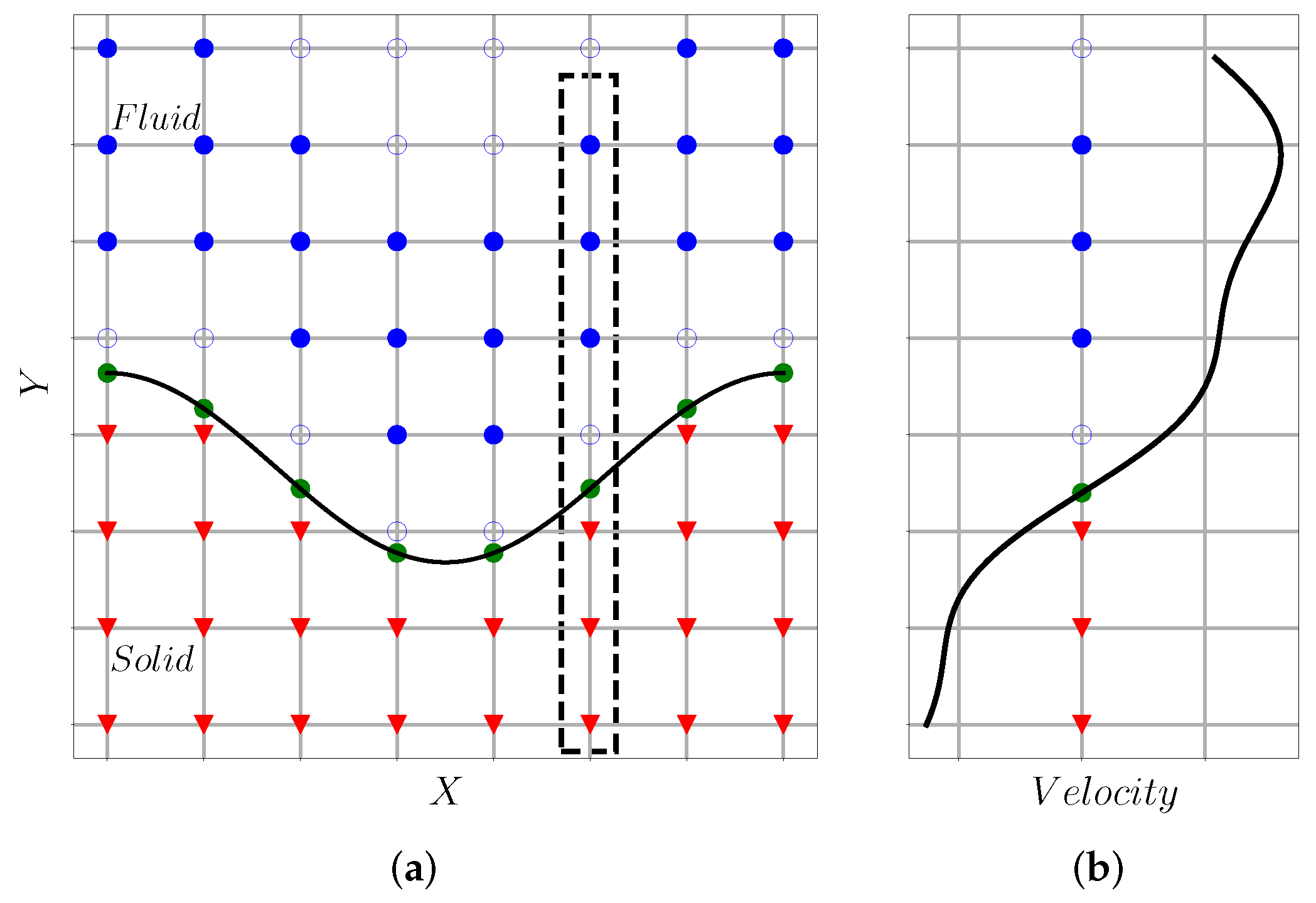
A major downside to the use of higher-order schemes as above is the representation of the complex geometry. In particular, the boundary conditions for higher-order methods are complex and hard to implement without loss of accuracy near the surface. In this work, we adopt an immersed boundary method (IBM) framework to represent the complex surface shapes. In the IBM the surface representation is accomplished through an added body force term to the governing equations while the background grid can be a simple Cartesian grid. Therefore, this approach saves significant grid generation effort, but is prone to inaccuracies. In this study, we leverage the higher-order IBM implementation in Incompact3D using the direct forcing method requiring reconstruction of the velocity field inside the solid region. This can be illustrated using the schematic in
Figure 1.
Figure 1a denotes the solid nodes in red, fluid nodes in blue, and the interfacial nodes in green. The solid curve represents the continuous shape of the fluid–solid interface.
Figure 1b shows local velocity variation along the
y direction corresponding to the black rectangle in
Figure 1a for illustration purposes. The IBM framework aims to enforce zero velocity at the interface through a velocity field reconstruction in the red solid nodes so that the higher-order (6OCCS) gradient computations can be estimated without sacrificing accuracy. Therefore, the key to the success of this approach is the velocity reconstruction step inside the solid region (red nodes in the schematic) using information at the blue and green nodes. To improve stability the grid point closest to the boundary (denoted by hollow circle) is ignored in the extrapolation step. The numerous different IBM implementations [
36] differ in the details of this velocity reconstruction. In the current study, we adopt the one-dimensional higher-order polynomial reconstruction as reported in the work by the authors of [
38]. This reconstructed velocity field is directly used to estimate the derivatives in the advection and diffusion terms of the transport equation. An illustration of this approach is shown in
Figure 1b. Using this 1D polynomial reconstruction, one estimates different solid region velocity fields when computing the derivatives along the different directions (x, y, and z). This is an advantage as well as a disadvantage. However, for the purposes of this study, this approach has shown to be reasonably accurate as described in
Section 2.3.
2.1. Simulation Design
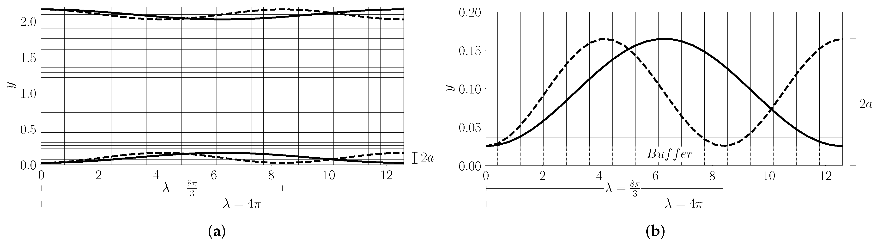
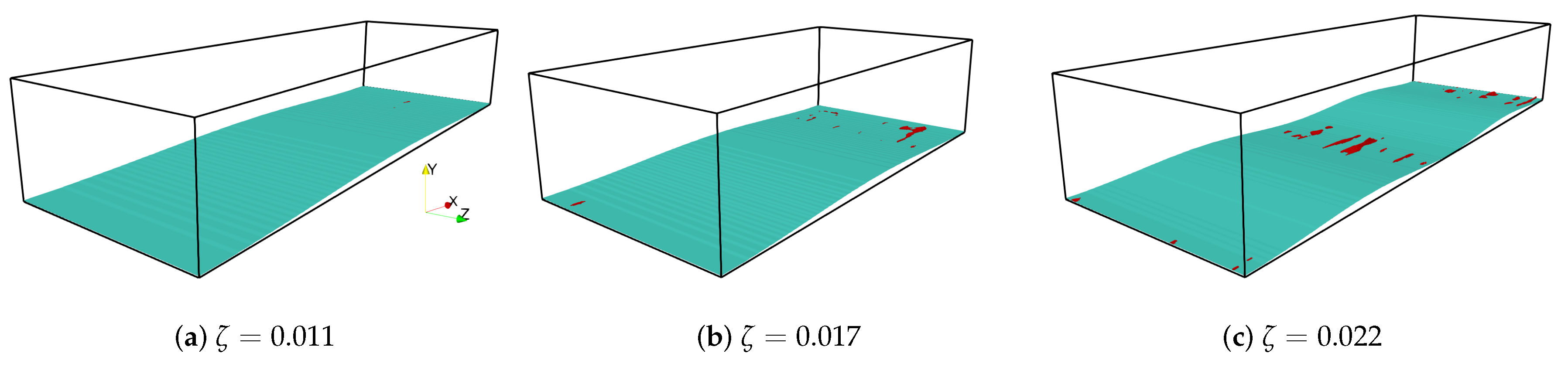
We carry out four different simulations of turbulent flows in flat and wavy channels with different steepness levels (
), but with the same peak wave height (
a) as shown in
Figure 2a. We define an average wave steepness,
, where
is the wavelength. In our study
varies from 0 to 0.022 corresponding to zero, one , one-and-one-half, and finally, two waves over the streamwise length of the domain. For all these cases, care was taken to ensure that the friction Reynolds number is maintained to a nearly constant value of ~180. The corresponding bulk Reynolds number,
, for the flat channel case is ~2800. For the wavy channel turbulent flows with the same effective flow volume and mean channel heights, maintaining the same flow rate (or bulk velocity) increases the corresponding friction Reynolds number,
, due to increase in
with wave steepness,
. However, this increment is at most ~10% in the current work and is not expected to influence our analysis significantly. The simulation parameters for the different cases are summarized in
Table 1. The simulation domain is chosen as
(including the buffer zone for the IBM) where
is the boundary layer height. This volume is discretized using a resolution of 256 × 257 × 168 grid points. In the streamwise and spanwise directions, periodic boundary conditions are enforced while a uniform grid distribution is adopted. In the wall normal direction, the no-slip condition representing the presence of the solid wall causes inhomogeneity. To capture the viscous layers accurately, a stretched grid is used. The grid stretching in the inhomogeneous direction is carefully chosen using a mapping function that operates well with the spectral solver for the pressure Poisson equation. The different inner scaled grid spacings are also included in
Table 1.
We note that the current analysis tries to balance three issues:
The major focus of the current work is on slope-dependent dynamics without presence of significant separation. This is part of a broader analysis theme where we expect to characterize how separation related dynamics impact turbulence structure differently from when significant separation exists.
At the same time, we wanted to realize high enough Reynolds numbers to characterize well known turbulent behavior, and yet,
minimize computational/storage cost.
The Reynolds number at which sustained separation will occur tends to reduce with increased steepness (). Therefore, if one were to consider higher Reynolds number, we expect to reduce the range of considered in the analysis which in turn requires very high grid resolution (and computational cost) to resolve the thin viscous layers. That said, modeling higher Reynolds numbers subject to availability of compute resources is a potential future work.
2.2. Convergence of Turbulence Statistics
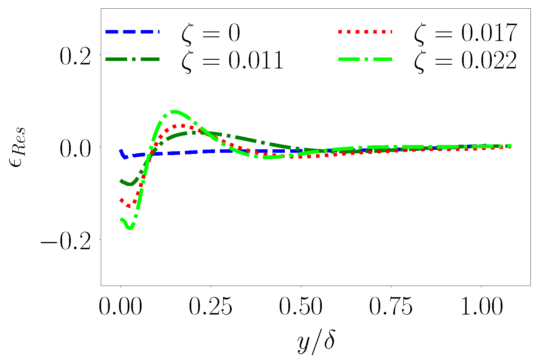
In order to quantify the convergence of the simulation and ensure statistical stationarity of the turbulence, we consider the streamwise component of the inner scaled mean spatial and temporally averaged horizontal stress that includes both the mean viscous and Reynolds stress components as
. Here,
represents the averaging operation with subscripts denoting averaging directions. In the limit of statistically stationary and horizontally homogeneous turbulence,
can be approximated to a linear profile,
as derived from the mean momentum conservation equations. We estimate a residual convergence error
as
whose variation with
is shown in
Figure 3.
We note that this error is sufficiently small for the flat channel () with magnitudes approaching 0.01 near the surface and much smaller in the outer layers. The plot also shows similar quantifications for wavy channel turbulence data with large residual errors near the surface. This is not surprising given that closer to the wall, the turbulence structure is known to deviate from equilibrium due to deviations from horizontal homogeneity. In fact, such deviations from equilibrium phenomenology will be expounded further in the later sections of the article. Nevertheless, we show here that farther away from the surface, the mean horizontal stress approaches equilibrium values as an indicator of stationarity.
2.3. Assessment of Simulation Accuracy
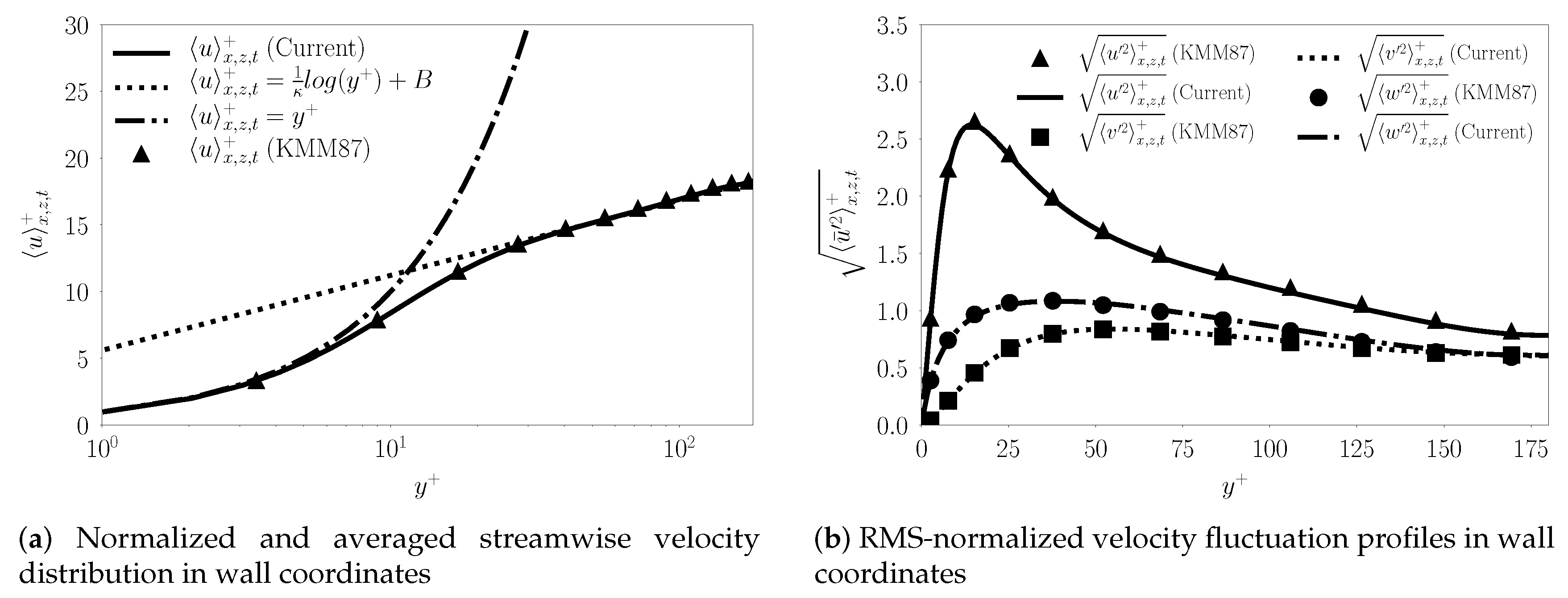
We perform a baseline assessment of the computational accuracy for the turbulent channel flow using an immersed flat channel surface before adopting it for more complex surface shapes. We compare the mean and variance profiles from the current DNS of immersed flat channel flow with the well known work of Kim, Moin, and Moser [
39] (KMM87 henceforth). This turbulent channel flow corresponds to a bulk Reynolds number,
, mean centerline velocity Reynolds number,
, and a friction Reynolds number,
. KMM87 used nearly
(128 × 129 × 128 grid points and solved the flow equations by advancing modified variables, namely, wall-normal vorticity, and Laplacian of the wall-normal velocity without explicitly considering pressure. They adopted a Chebychev-tau scheme in the wall-normal direction, Fourier representation in the horizontal and Crank-Nicholson scheme for the time integration. In our work, we adopt a spectrally accurate 6th-order compact scheme in space and a third order Adam–Bashforth time integration as reported in the work by the authors of [
34].
Figure 4 clearly shows that the inner-scaled mean (
Figure 4a) and root mean square of the fluctuations (
Figure 4b) from the current simulations match that of KMM87. We observe slight differences for the streamwise velocity fluctuation RMS in the outer layer which can be attributed to the improved resolution (and accurate time integration) in our simulations. The method employs a staggered grid arrangement for improved mass conservation.
3. Results
The primary goal of this study is two-fold: (i) to explore the nonequilibrium, near-surface turbulence structure over systematically varied sinusoidal undulations and (ii) characterize the roughness characteristics of such wavy surfaces. In addition, wherever possible, we quantify deviations from equilibrium phenomenology as evidenced in flat channel turbulence, assess the extent of outer layer similarity, and relate to characteristic roughness induced effects as appropriate. To accomplish this, we use conventional turbulence quantifications such as mean first- and second-order statistics (velocity variances and turbulent kinetic energy (TKE)), horizontal flow stress, and mean nondimensional velocity gradient profiles. As discussed in
Section 2.1, we consider four different steepness (
) levels (
Table 1), including the flat surface to understand the impact on turbulence structure. The flat channel with
represents equilibrium turbulent flow due to horizontal homogeneity and stationarity. To contrast, we consider turbulent flows over wavy surfaces with very little separation as shown in
Figure 5.
The analysis can be realized using both instantaneous as well as averaged turbulence structure. In this article we focus on the streamwise-averaged or more commonly known as the ‘double-averaged’ turbulence structure which is a function of solely the wall normal distance. The term ‘double-averaging’ refers to the combination of averaging along homogeneous () and inhomogeneous (x) directions. For the spatial averaging, we include both streamwise (x) and spanwise (z) spatial directions, and for the temporal (t) averaging, we include 2500 three-dimensional snapshots over 20 flow through times for the chosen friction Reynolds number. We use the notation to specify a quantity u being averaged over x, z, and t. For the flat surface, horizontal homogeneity and stationarity implies that x, z, and t are equivalent in the averaging operation, (i.e., generate equivalent results in the limit of sufficient samples). However, when dealing with two-dimensional non-flat surfaces as in this work, only z and t are equivalent and provide the same results, but depend on x due to absence of streamwise homogeneity near the surface. Therefore, in such situations it is only natural to consider averaged quantities that have both streamwise (x) and vertical (y) variability. This allows one to characterize the near-surface inhomogeneity along both directions. However, in order to quantify deviations from equilibrium and assess the impact of near-surface inhomogeneity on the turbulence we consider streamwise averaged statistics.
3.1. Streamwise Averaging of Turbulence Statistics
In this section, we focus on the deviations from equilibrium in turbulence structure using streamwise averaged statistics that depend only on and .
To average along the wavy surface, we define a local vertical coordinate, at each streamwise location with at the wall. Its maximum possible value is the mid channel height and changes with streamwise location. We then perform streamwise averaging along constant values of to generate mean statistical profiles. A slight variant of the above is to use a rescaled coordinate which stretches everywhere between where is the mean half channel height. One averages over constant values of to generate another set of double-averaged mean statistics. Both approaches implicitly approximate the terrain as nearly flat with a large radius of curvature in a local sense and therefore, nearly homogeneous. This approximation works well when . In our study which is an order of magnitude larger than the typical viscous length scale, , but smaller than the log layer () with strong inertial dynamics.
For the mean velocity results presented in this section, we compare both the averaging approaches to illustrate their closeness to each other. Specifically, we use thick solid lines to denote the mean profiles averaged over constant local coordinate
and thin lines with markers to denote averaged quantities using scaled local coordinate
. However, for the rest of our analysis, we average over
in a manner consistent with the literature although a second possibility exists. Furthermore, the results from the two approaches are close enough to each other (
Figure 6) to not warrant two different approaches for this analysis. The different colors, namely, blue, green, red, and lime are associated with different wave steepness,
,
,
, and
, respectively.
3.2. Outer Layer Similarity and Mean Velocity Profiles
As the mean channel height (for wavy geometry) is kept constant across all different steepness,
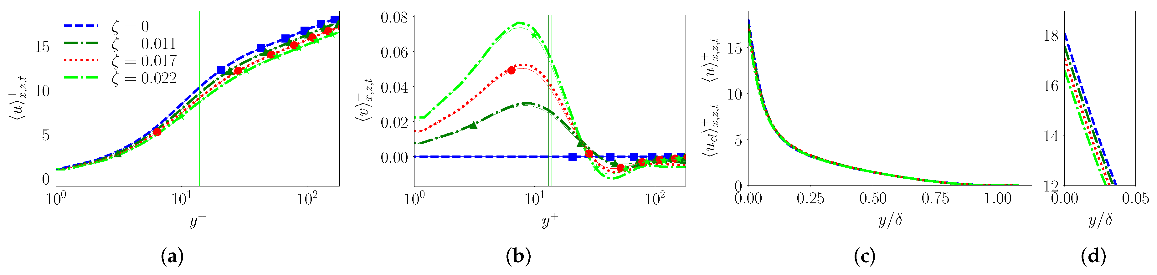
, the observed changes in the mean statistics are only due to surface effects and not the outer layer dynamics. In
Figure 6, we show the inner-scaled, double-averaged streamwise and vertical velocity for the different cases. The prominent observation for the streamwise velocity is an upward shift (downward shift in the
plot) with increasing wave steepness,
(
Figure 6a), which increases with
before showing near linear growth in the log-layer. This trend is well known for rough-wall turbulent boundary layers [
16] and is indicative of slowing down of the flow near the wall from increased drag due to the wavy surface for a fixed mass flow rate (bulk Reynolds number). This would naturally result in higher centerline velocities and
as seen in
Table 1 in order to maintain the prescribed flow rate. The vertical mean velocity structure (
Figure 6a) is consistent with this interpretation as the wavy undulations generate increasingly stronger net vertical velocity close to the surface with increase in
. As seen from
Figure 6a, the mean vertical velocity profile shows systematic upward flow in the viscous and buffer layer along with a weak downward flow in the logarithmic region in order to maintain zero net flow in the vertical direction. It is well known that the mean vertical velocity is zero due to horizontal homogeneity for the flat channel (
). Therefore, these well-established vertical motions in the mean over wavy surfaces, although small (
), represent the most obvious form of deviations from horizontal homogeneity, a prerequisite for equilibrium.
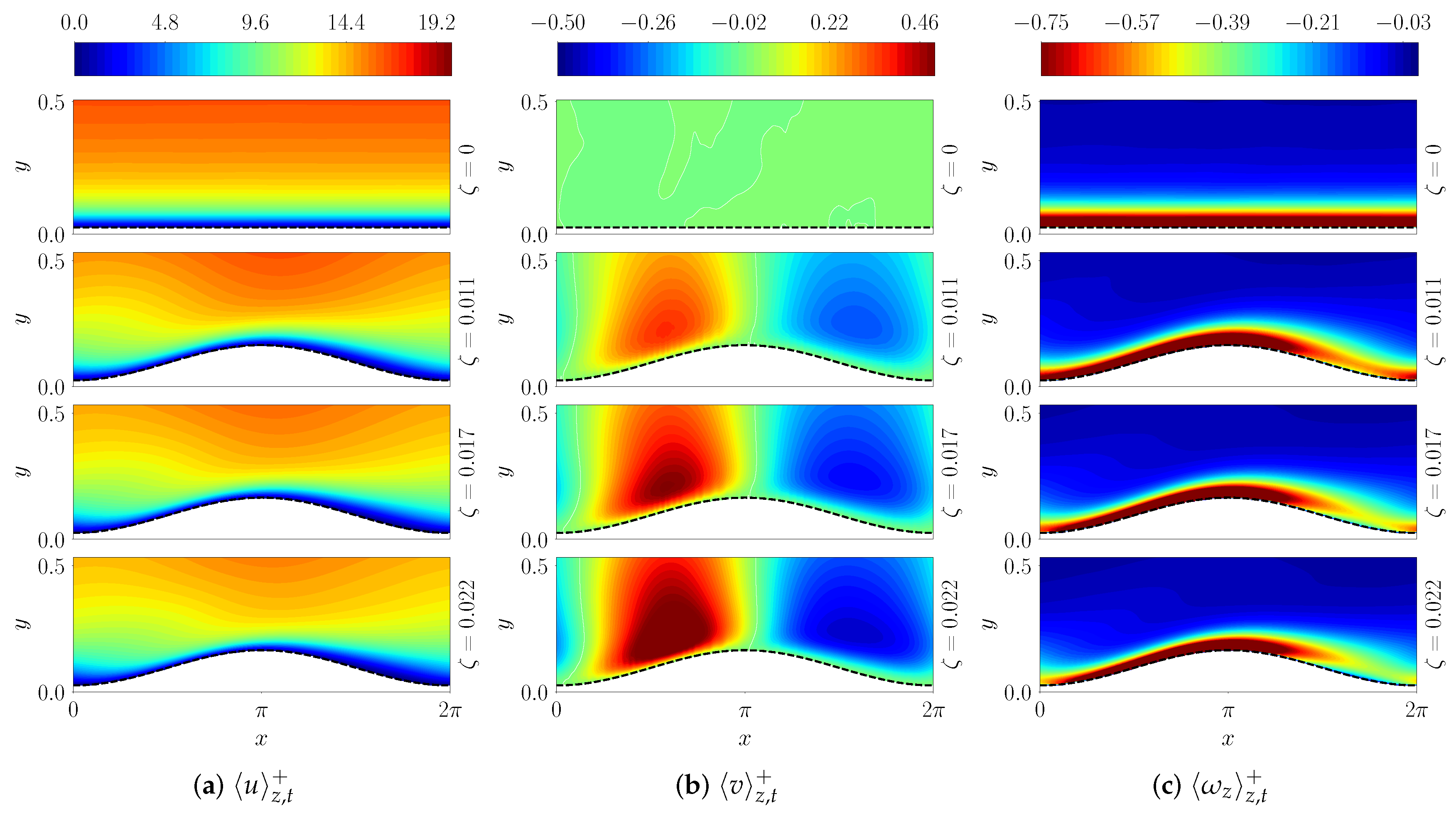
In particular, the vertical velocity is asymmetric with respect to the symmetric wavy shape as seen from isocontours of time-averaged mean vertical velocity shown in
Figure 7. We observe that the upward and downward slopes display varying tendencies due to presence of adverse and favorable pressure gradients, which decelerate (push the flow upward) and accelerate (push downward) the flow as expected. However, the extent of upward deceleration dominates the downward acceleration which breaks the symmetry of the flow patterns around the wave crest. This asymmetry increases with
resulting in stronger net vertical flow in the lower buffer layer (
Figure 6a).
A better insight into the steepness dependence of this asymmetry can be gained by investigating the averaged structure of spanwise vorticity (
) as given by
. As illustrated in
Figure 7c, the spanwise vorticity is predominantly attached to the surface in the upslope region for different
, which is qualitatively reminiscent of a flat surface. However, the thickness of the strong vorticity region shows streamwise dependence. However, in the downslope region, the region of strong vorticity exists away from the surface indicating lifting of the shear layer at higher
. This suggests incipient flow separation in the mean although intermittent flow separation exists (
Figure 5) for all the non-zero
considered in this work. This separation however is not consistent enough to show up in the mean statistics. Such incipient separation can be interpreted as the streamwise gradient of vertical velocity (
) approaching the vertical gradient of streamwise velocity (
) at higher values of
closer to the surface. At higher steepness, the shear layer is expected to completely detach from the wall and a layer of positive vorticity is expected to emerge underneath in an averaged sense due to strong and consistent separation downslope of the peak.
In spite of these near surface deviations, the dynamics outside the roughness sublayer tend to be similar when normalized and shifted appropriately. To illustrate this outer layer similarity, we show the defect velocity profiles in
Figure 6b that indicate little to no deviation between
and
. If anything, the deviation is slightly higher near the surface in the roughness sublayer, as illustrated in
Figure 6c.
3.3. Quantification of Mean Velocity Gradients and Inertial Sublayer
The normalized mean streamwise velocity gradients identify the different regions of the turbulent boundary layer and are especially useful to quantify the extent of the inertial sublayer (or the logarithmic region) and the von Kármán constant. In this study, we estimate the normalized premultiplied inner-scaled mean gradient
, as shown in
Figure 8a. This function achieves a near constant value of
(where
is the von Kármán constant) in the inertial sublayer due to normalization of the mean gradient by characteristic law of the wall variables, i.e., surface layer velocity (
) and distance from the wall (
y). In this study, for the chosen bulk Reynolds number,
(and the realized narrow range of friction Reynolds numbers,
) we observe that the inertial layer exists over
for
which shifts to
for
. At the outset, this upward shift (rightward in the plot) in the log layer appears to be associated with the change in wave steepness,
and not the small changes (~10% or lower) in friction Reynolds number,
. In this context, we refer to the work of Moser et al. [
40], who show that similar shifts in the logarithmic region occur only over significant changes in Reynolds number, much larger than the variations observed in this study. The estimated von Kármán constants are tabulated in
Table 2, and show a range of 0.38 to 0.40 for the different runs. In this study, we use the appropriate value of
to compute the different metrics.
A related quantification often employed to interpret near wall structure is the nondimensional mean streamwise velocity gradient,
whose variation with inner-scaled wall normal distance is shown in
Figure 8b. It is easy to see that
. We observe that the
profiles for different
mimic the characteristic equilibrium structure starting from zero at the wall followed by a peak at the edge of viscous layer and subsequently, a gradual decrease in the buffer layer to a value of one in the inertial sublayer. The deviations from surface layer similarity in
for
clearly indicates the increasing influence of outer layer scales in that region. This is easily verified from the outer layer similarity observed in
Figure 6b. In fact, there exists an overall shape similarity in
hinting at the potential for universality if only the appropriate scales at the different regimes can be identified.
The origin of the ‘overshoot’ or near-surface peak is well known and is related to the inconsistency from normalization of the mean gradient using inertial scale variables closer to the surface (viscous layer) where the physically relevant characteristic length scale is . With some analysis, one can easily show that undergoes a linear growth as near the surface ( being a constant). In the buffer layer, one can similarly formulate , with increasing super linearly and with y to cause the peak followed by a decrease as one approaches the inertial sublayer. In the inertial layer, with varying linearly with y as per law of the wall (resulting in and assuming constant values).
In this context, we see that as the friction velocity,
increases with
(see
Table 1), the viscous length scale,
decreases resulting in faster growth of
in the viscous layer, but over a smaller height that scales with
. This is consistent with
Figure 8a,b which show that the magnitude of the peak at the viscous-buffer layer transition decreases with increase in
. In addition, we observe an upward (rightward) shift in the log region (i.e., region of nearly constant
and
) with
. Taken together, the above observations, namely the upward shift in the log region (
Figure 8a) and the smaller peak in
with increase in
, indicate that the buffer layer becomes increasingly thicker for steeper waves. The ‘buffer layer’ is known as a region of high turbulence production [
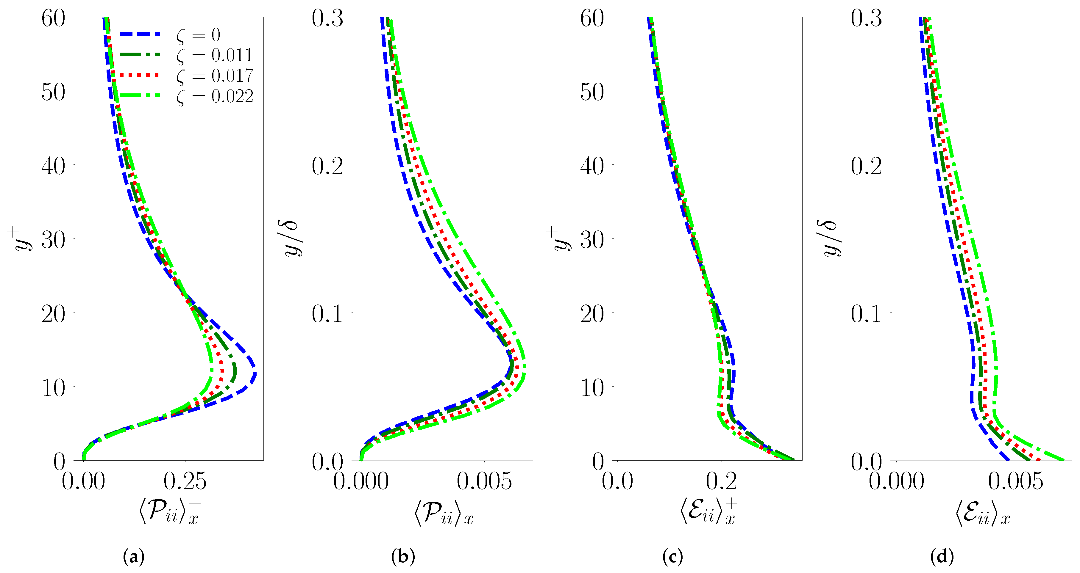
41], where both the viscous and Reynolds stresses are significant. Therefore, the expansion of the buffer layer with
is a consequence of the turbulence production zone expanding due to the wavy surface. This is evident from
Figure 9 where the decay in turbulence kinetic energy (TKE) production is slower for higher
in the buffer region (
) in both inner-scaled (
Figure 9a) and dimensional (
Figure 9b) forms. A consistent trend is observed in the TKE dissipation which is known to peak at the wall before decreasing sharply with height in the surface layer while undergoing relatively little change in the buffer layer increasingly dominated by inertial dynamics before decreasing gradually away from the surface. The inner scaled dissipation profiles (
Figure 9c) clearly suggest that at higher
the region of nearly constant dissipation (corresponding to buffer layer dynamics) is more pronounced and extending over a larger region of the TBL. In addition, the normalized dissipation rate is smaller for higher
. We expect this trend to be even stronger in the presence of significant separation at larger values of
. This trend is consistent with prevalent understanding of classical rough wall boundary layers at high Reynolds numbers, especially in the lower atmosphere where the roughness elements of size
tend to completely destroy the viscous layer [
16], if not most of the buffer layer. In our studies,
for the different
(see
Table 1) and only modulates the buffer layer. A related observation is that the vertical location of the inner scaled peak turbulence production (
) does not change with
, but the magnitude decreases. This is not surprising as for
, there exists other sources of turbulence generation, i.e., from the surface roughness or undulations which contributes to the total friction.
3.4. Characterization of the Roughness Function and Roughness Scales
A common way to assess the influence of the wavy surface on turbulence structure is to quantify the effective drag and its influences on the flow structure. While the increase in friction velocity for a fixed
(apparent from
Table 1) is a natural way to quantify the increased drag, estimating the downward shift in the mean streamwise velocity profile (
Figure 6a) is another approach and often used to characterize the effective roughness scales. It is well known that the logarithmic region in the equilibrium flat channel turbulent boundary layer (TBL) is given by
where the additive constant B is typically estimated to fall within the range of ~5.0 to 6.0, and depends on the details of the buffer and viscous layer for a given simulation or measurement. The flat channel data in the current work provides an estimate of ~5.6, possibly due to a combination of the friction Reynolds number regime and simulation algorithm. In the presence of surface undulations of scale
a, we observed from the earlier discussion that the log region underwent a upward shift due to an expanding buffer layer. As per the works by the authors of [
13,
16,
25], the influence of these buffer layer modulations on the log layer shift is characterized in terms of a modified logarithmic profile for rough-wall turbulent boundary layers (TBLs),
where
is defined as the roughness function. The roughness function,
can be related to the characteristic ”equivalent” sand grain roughness,
as
and the characteristic roughness length,
as
It is easily seen that
. While
and
are used to quantify the nonequilibrium ’roughness’ effects near the surface, they mostly cater to complex roughness such as grasslands, urban canopies, or sand grain type surfaces. Of course,
corresponds to a case where the buffer layer dynamics is significantly modified by the roughness, while
corresponds to a situation where the buffer and viscous layers are completely destroyed by the roughness. Therefore, such metrics do not represent the smooth, low steepness surfaces adopted in this work.
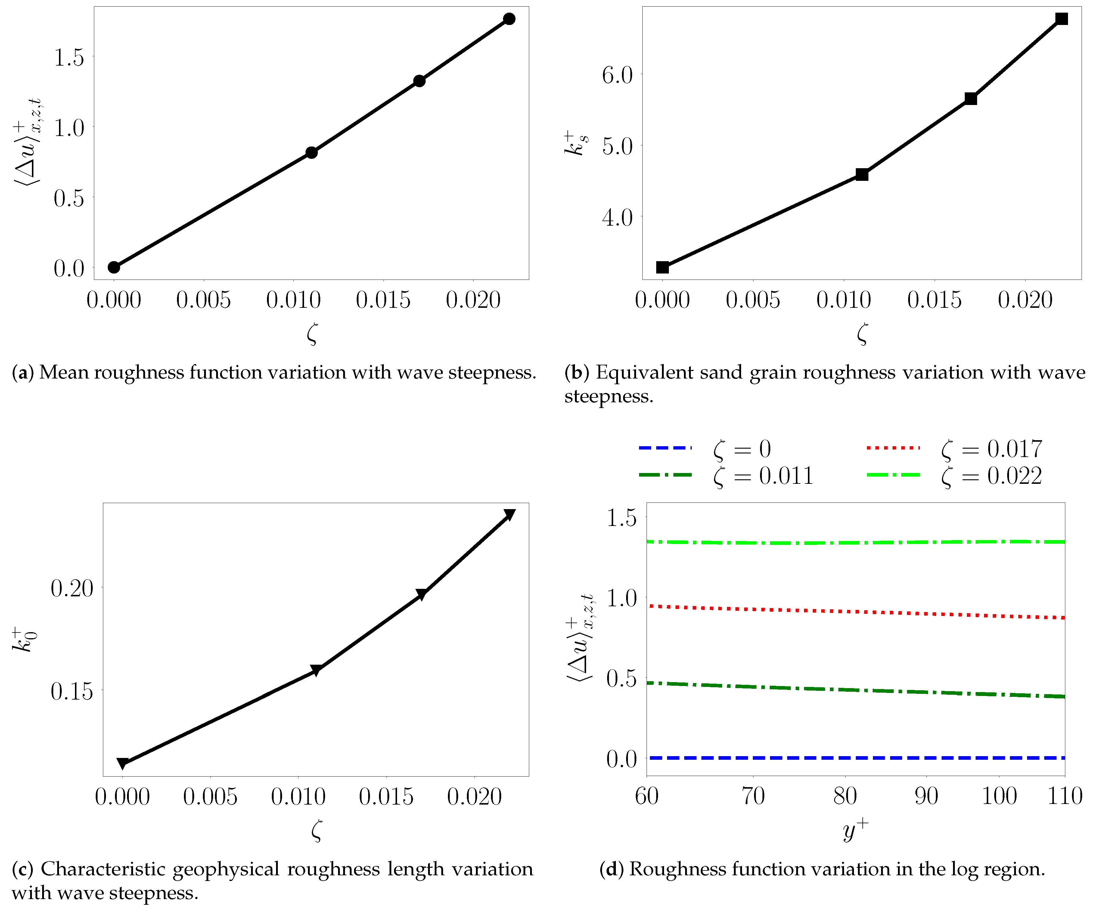
Table 2 compiles estimates of the roughness function,
, averaged over the entire logarithmic region given by
60–120 as illustrated in
Figure 10d over which the values are nearly constant. For all the metrics reported in this work, we use data from the averaged profiles across constant values of the nonscaled local coordinate,
.
For comparison sake, we also report the equivalent sand grain roughness,
of Nikuradse [
3] and the characteristic roughness length,
scaled by the inner-layer variables for different values of
. As expected, these different roughness metrics increase linearly with wave steepness as seen in
Figure 10a–c. The effective sand grain roughness assumes a non-zero value of ≈3.3 for
due to the upward shift caused by the viscous and buffer layers. Therefore,
is indicative of a nearly smooth wall which in our study corresponds to
0–0.01. The higher values of
considered in this work generate
although no substantial flow separation is observed. As expected, the
is extremely small indicating that the flow is smooth enough to retain the viscous and buffer layers.
Given that
is nearly constant for all the cases while
and
show near linear growth confirm that such wavy surfaces do not fit the
k-type roughness description [
16,
42]. In addition, given that the boundary layer height in fully developed channel flow turbulence is fixed as a constant
, the independence of
on
indicates a departure from
d-type classification [
42]. In fact such surfaces as considered in this work belong to the ‘transitional’ and ‘waviness’ regime as
does not represent a sufficiently large (i.e,
) roughness Reynolds number,
. We have also reported the
values for the different cases in
Table 1 and
Table 2.
The ‘waviness’ regime implies a surface that is very different from a Nikuradse roughness dominated by form drag caused by flow separation and vortical recirculation zones within the roughness sublayer. Therefore, strong waviness causes the drag (as estimated by the roughness function
) to be smaller than the corresponding Nikuradse value for a given
. At low slopes (waviness) the overall drag is more dominated by viscous shear and less by the form drag. The opposite is true in the roughness regime. This is clearly illustrated in
Figure 11a, where the correlation between
and
from Nikuradse [
3] and Colebrook [
4] are compared with our current DNS data. We clearly see that for the current study with nearly constant
,
increases with wave steepness
which we anticipate will approach the corresponding value for a sand–grain roughness with similar roughness Reynolds number,
(or the Nikuradse value for this
). However, verifying this requires additional simulations at high
and possibly, other values of
. The wave slope dependence on the flow drag is evident from
Figure 11b, where
is shown against the effective slope, ES
.
Figure 11b also shows the data from Schultz and Flack [
12], who performed experiments with systematically varied pyramid roughness elements of different slope. These data trends indicate that the slope transition from waviness to Nikuradse type roughness regime (denoted by a vertical line in
Figure 11b) occurs between
0.25–0.4 (
0.12–0.18) with possible dependence on the extent of separation between the surface and outer layer scales (
) and Reynolds number (
). This transition has been correlated to the dominance of form drag over viscous drag [
12,
17]. We note that our data from the reported simulations closely follow the trend of Napoli et al. [
17], i.e.,
increases with ES. As stated earlier, we anticipate this increase to cap at a value of
corresponding to a sand–grain roughness Reynolds number,
. Although this extrapolated trend is consistent with the observed experimental data [
12], it needs to be verified through additional simulations at larger
. If this is indeed true, then the capping value of
for the fully rough case (with high effective slope surface) can be estimated from the Nikuradse correlation [
3] for sand grain roughness (denoted by the horizontal line in
Figure 11b for our DNS data). For the benefit of the reader, we have explicitly documented the roughness function correlations of Nikuradse and Colebrook used above in
Appendix A.
In summary, the modulations in the mean-averaged first-order statistics from wavy surface undulations manifest as (i) increase in drag (through friction velocity ) and a (ii) modified buffer region including (iii) a systematic upward flow in the buffer layer and a smaller downward flow at the lower logarithmic layer. To interpret the above effects better, we analyze the horizontal flow stress and components of the Reynolds stress tensor in the following sections.
3.5. Characterization of Horizontal Flow Stress and Implications to Drag
The horizontal flow stress directly impacts the flow drag through the boundary layer and in turn the mean velocity profiles discussed above. The viscous flow stress acting on a fluid particle is described including both spanwise and streamwise components as , where and . Similarly, the Reynolds stress is given by , where and . The total horizontal stress is then with without overbars denoting their magnitudes.
Figure 12a shows the inner-scaled double-averaged horizontal stress magnitude,
felt by a fluid particle. We further split this into the inner-scaled viscous and turbulent parts,
respectively as shown in
Figure 12b,c. In the viscous layer, the total stress is dominated by the viscous stress for the different cases A-D with different
varying between 0 and 0.022. The inner scaled mean viscous shear stress magnitude (
Figure 12b) decreases with steepness (
Figure 12b) in the viscous layer where it is nearly constant before decreasing across the buffer layer. Away from the mean surface level, in the buffer layer, the inner-scaled Reynolds stress magnitude grows (from near-zero values in the viscous layer) into a peak value at
(
Figure 12c) whose magnitude increases with
before collapsing over each other in the log layer. Overall, the viscous stress dominates in the viscous layer while the Reynolds stress grows through the buffer layer (a region where the viscous stresses continually decrease in importance) to peak at the buffer–log transition region.
The decrease in magnitude of the inner-scaled viscous stress with
in the viscous and lower buffer layers is a consequence of the normalization using the averaged wall stress,
which increases with wave steepness. We observe that the mean
is relatively unaffected, but its contribution to the total drag decreases with increase in
. In general, the mean streamwise flow near the wall slows down due to the presence of wave-like undulations (see
Figure 6a), which in turn reduces its gradient in the wall normal direction. This reduction in the average viscous stress is compensated by the non-zero vertical velocity and its variation along the streamwise and vertical direction. This explains why the net double-averaged (i.e., both temporally and spatially averaged) dimensional viscous stress sees very little increase in the viscous layer as seen from the dimensional stress profiles in
Figure 12e. This observation clearly indicates that the increase in net wall stress (
) with
has its origins in the increase of Reynolds stress in the buffer–log layer transition as seen in
Figure 12f which is reflected in the total mean stress variation as well (
Figure 12d). Given that the nondimensional roughness scale,
corresponds to the buffer layer, it is not surprising that the buffer layer shoulders much of the effect of increasing wave steepness. However, the mechanism underlying increase in the peak double-averaged Reynolds stress with
will invariably depend on the structure of the attached (or detached) shear layers in the vicinity of the wavy surface resulting in a coupling between the viscous shear layers and buffer layer turbulence production. The nature of this coupling will be further explored in the future. Of course, when the shears layers are detached as in a separated flow, the interactions could entail very different characteristics.
3.6. Characterization of Reynolds Stress Tensor and its Production
In the earlier discussions, we focused on the mean gradients and their impact on the horizontal flow stresses. In this section, we focus on the effect of changing
on elements of the Reynolds stress tensor and the turbulent kinetic energy that are borne out of the interaction between mean gradients and the Reynolds stress. We observed earlier (
Figure 8) that the peak in the mean gradients at the start of the buffer layer decreases with surface undulations, which also impacts turbulence production (
Figure 9) in the lower buffer layer and, in turn, the individual components of the Reynolds stress tensor
.
3.6.1. Streamwise Variance
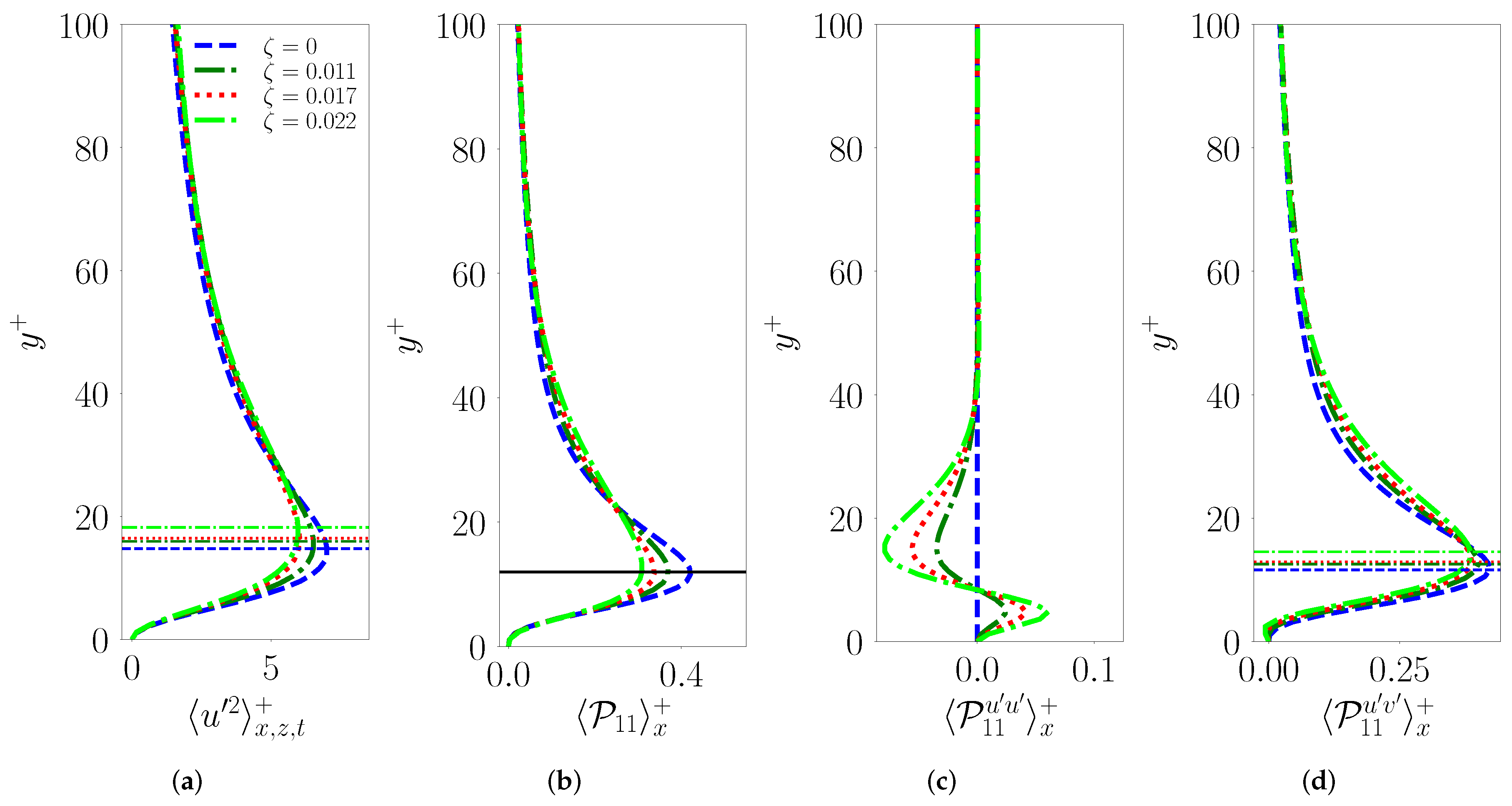
In fact, the most noticeable deviations from equilibrium in wavy wall turbulence occur in the second-order statistics. In particular, we observe in
Figure 13a the inner-scaled streamwise variance that peaks in the buffer layer and this peak value decreases with increase in
. In addition, the inner scaled profiles nearly collapse in the outer region for all
, while the location of peak streamwise variance shifts upward as
increases. Given the lack of significant flow separation, this upward shift in the peak variance is modest, but noticeable. We identify the peak location for each curve with color-matched horizontal lines so that the trends can be identified. Using this, we see a systematic upward shift of the peak value of
with
in
Figure 13a. Related research by Ganju et al. [
43] showed that this upward shift is tied to significant increases in roughness scale,
, which can cause very different dynamics around the wave including flow separation. Further, the effect of changing
was reported to be minimal in their investigation. Their first observation is consistent with classical understanding of high Reynolds number rough wall turbulence [
16,
41], where the peak variances occur at nearly the roughness height,
a. In fact, wall stress boundary conditions for large eddy simulation over rough surfaces are designed to model the same. In our study, the amplitude,
a is fixed while the wavelength
is decreased in order to change
. For a fixed bulk Reynolds number, the decrease in
(or increase in
) increases the net drag, and in turn the friction velocity,
. The resulting decrease in the viscous length scale,
changes the inner-scaled wave height,
rather modestly from 13.07 to 13.92 when
doubles from
(see
Table 2). Therefore, this systematic upward shift in the location of peak streamwise variance cannot be solely attributed to these very modest increases in
. In fact, the wave steepness significantly impacts the buffer layer dynamics and in turn the variance distribution through the turbulence production mechanisms as delineated under.
We further dissect the above observations using the variance production (
Figure 13b) term
, in the Reynolds stress transport equation. Note that we further split this component variance production into its dominant contributions,
and
as shown in
Figure 13c,d, respectively. We clearly observe that the inner-scaled streamwise variance production due to interaction of the scaled mean shear (i.e., inner-scaled vertical gradient of the mean horizontal velocity,
) with the vertical momentum flux (
) denoted by
clearly peaks in the buffer layer (
as seen in
Figure 13d), and this peak shifts upward (with minimal change in magnitude) for increasing
. This trend can be interpreted through the double-averaged profiles of normalized covariance
and mean gradient,
, respectively as shown in
Figure 14a,c. It is to be noted that
peaks at the edge of the buffer layer at
, whereas the normalized mean gradient achieves its maximum value near the surface. In addition, the location of the peak in
(at
) shows very little variation with no clear trend, but its magnitude increases with
all through the buffer and log layers. Contrary to this, the magnitude of
decreases with
due to surface undulations, whose influence decreases away from the surface (through the viscous and buffer layers). In summary, we understand that the combined influence of the surface-induced trends in
and
yields the trends observed for
, as shown in
Figure 13d, with peak values occurring over
for different
. In addition, the surface undulations play a secondary role in the variance transport (see
Figure 13c) with significant production in the roughness sublayer (
) followed by destruction above the roughness scale,
that decays with height. This production and destruction process clearly represents deviation from equilibrium as its origins lie in the streamwise mean velocity gradient,
being non-zero from horizontal inhomogeneity. A key consequence of this inhomogeneity driven destruction process is that both the peak inner-scaled variance production and the peak variance decrease with
(
Figure 13a). However, it also turns out that the systematic upward shift observed for the peak in
is nonexistent for the
profiles (the peak occurs at or around
), see
Figure 13b. In summary, we observe that more severe the surface inhomogeneities, smaller the rate of streamwise turbulence production through
,
, and
, but the location of peak production in wall coordinates remain unaffected. Therefore, the observed upward shift in the peak of
(
Figure 13a) should arise from other turbulent transport mechanisms including return to isotropy.
3.6.2. Vertical Variance
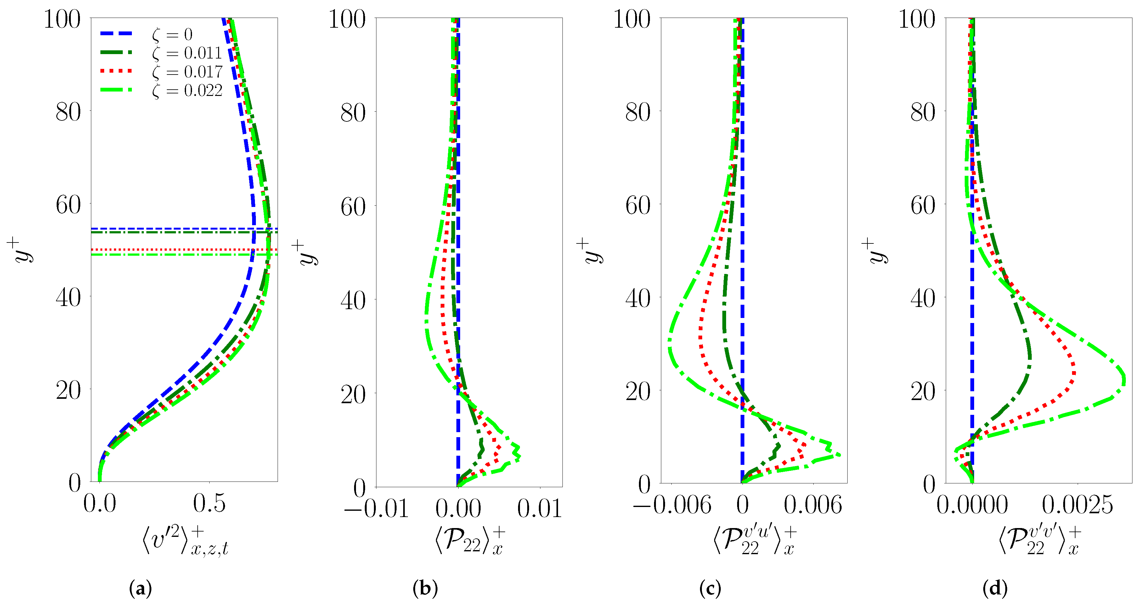
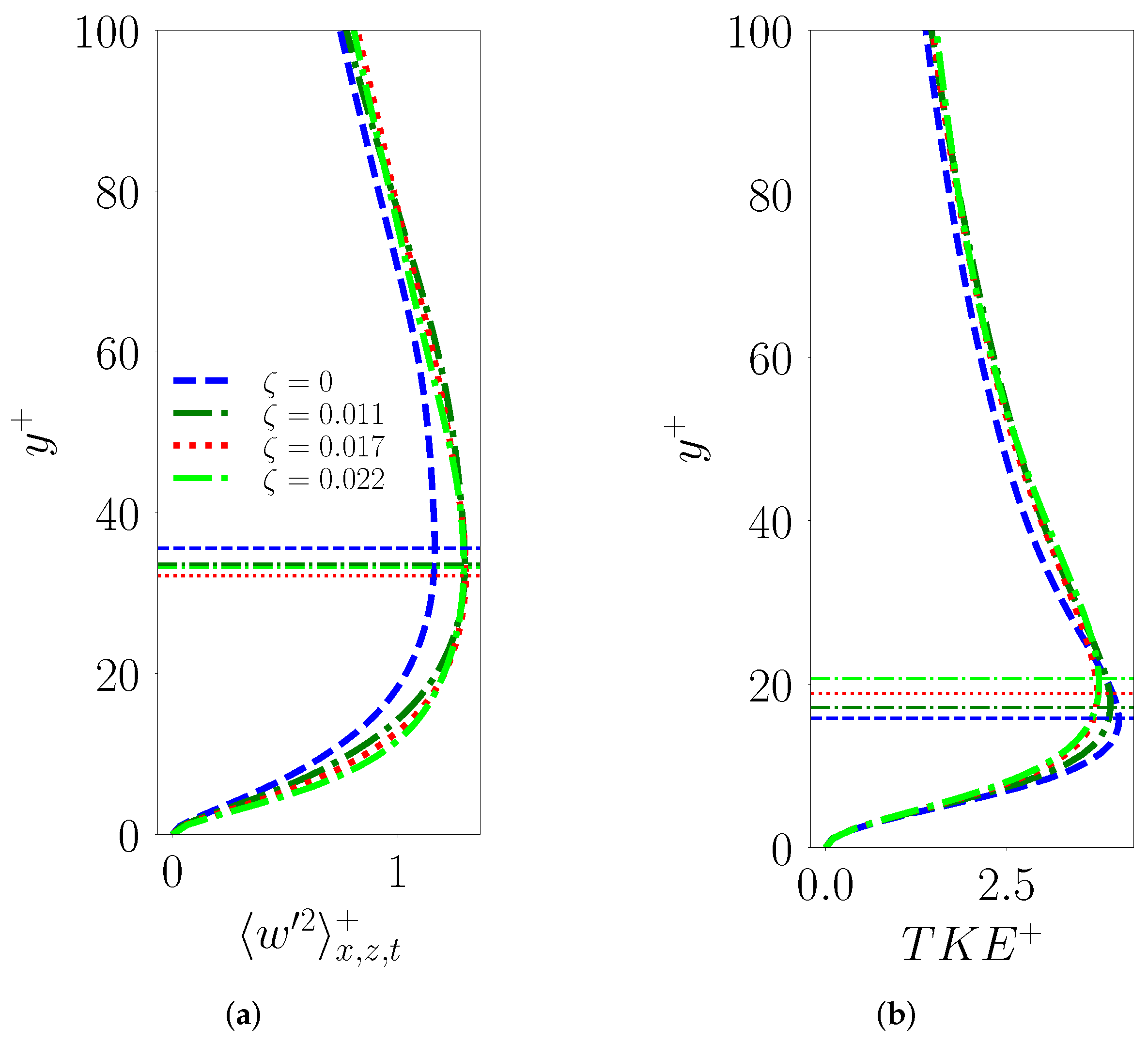
The effect of surface undulations on vertical variance profiles is opposite to that observed for the streamwise variance, i.e., the peak variance in the buffer–log transition region (
) increases and shifts downward with
in comparison to flat channel turbulence data. While the shift in the peak location is systematic, we note that the peak value in itself changes very little from
after making a sharp jump from
. It is well known [
41] that streamwise turbulent fluctuations are generated closer to the surface in the (buffer) layer, and is then distributed to the other components through the pressure–strain term [
44]. Consequently, the vertical and spanwise variances peak further away from the surface, closer to the log layer. Among the two, the vertical variance is nominally expected to achieve maximum value further away from the surface due to the wall effect, i.e., vertical fluctuations are damped closer to the wall. In our investigations, the vertical variance peaks closer to the log layer (
) while the spanwise variance peaks lower in the buffer–log transition (
) as observed in
Figure 15a and
Figure 16a respectively.
Due to the presence of surface undulations (non-zero
), vertical velocity variance is produced closer to wall (or effective wall for wavy surfaces) in the roughness sublayer (i.e,
) as seen from the inner-scaled vertical variance production,
in
Figure 15b. The extent of near surface production increases with wave steepness,
. To dissect further,
is further split into
and
as shown in
Figure 15c,d respectively. The dominant variance production originates from non-zero streamwise gradient of vertical velocity (see
Figure 6a) which is positive below the roughness scale and negative above it. Consequently, the surface imhomogeneity driven non-zero mean vertical flow over the wavy surface impacts turbulence production by generating vertical variance below the roughness scale and destroying some of it above in the buffer layer (
Figure 15c). Therefore, unlike flat channel turbulence, the return to isotropy is accelerated with increasing
, causing
to grow faster (
Figure 15a) through the viscous and buffer layers to ultimately peak closer to the surface (in the buffer–log transition). The location of peak vertical variance is illustrated in
Figure 15a through coloured horizontal lines that show a clear downward shift from
.
In essence, what we are observing is that changes in
with fixed
a impacts the growth rate in the buffer layer with perceptible effect on the peak location and magnitude. This trend is maintained until strong separation-related dynamics, including detachment of the shear layer, which sets in at higher
. As shown in Ganju et al. [
43], this causes a secondary peak in the buffer layer for both vertical and spanwise variance, possibly due to turbulence production within the separation bubble as well as above it. Such effects are absent in the current study as evidenced by just a single peak for the vertical variance production. While these observations are intriguing, it is not clear how these trends respond to the choice of Reynolds numbers, thus requiring further investigation. A limitation with increasing Reynolds numbers is that even relatively shallow surface undulations can produce separation which is known to perceptibly modulate the flow physics.
3.6.3. Spanwise Variance
Similar to
, the inner-scaled spanwise variance
also shows stronger growth (see
Figure 16a) through the viscous and lower regions of the buffer layer to ultimately peak in the buffer layer (
). Intriguingly, we note a systematic shift in the peak location and magnitude only for
, but little variation from
. This may be attributed to the peak occurring farther away from the surface where the inhomogeneity effects are small. As we are dealing with mildly steep two-dimensional wavy surfaces in this study, we observe that
is not produced near the surface as evidenced by the production terms in the variance transport equation (not shown here), being nearly zero throughout the boundary layer due to
. In spite of the quasi-two-dimensional wavy surfaces employed here, the above trends will breakdown in the presence of strong separation that can introduce three-dimensional flow patterns. As part of an ongoing research study we are exploring higher values of
to verify the above statement.
In the absence of three-dimensional flow (both forced by a three-dimensional surface and induced by separation over a two-dimensional surface), the location of peak
shows no clear monotonic trend although a consistent downward shift is observed for
. This can be attributed to either the small amounts of separation observed in these flows (see
Figure 5) or due to conversion of the vertical variance produced from the surface undulation through the pressure–strain term. We expect the latter to be the likely mechanism, although no quantification is provided work to support this hypothesis. As one would expect away from the surface, the
and
profiles across different values of
approach each other in the outer layer indicating that the effect of the surface undulations is concentrated closer to the surface. We nevertheless note that in this region of the TBL,
(
Figure 15a) and
(
Figure 16a) are slightly higher for non-zero
when compared to the flat channel with
.
3.6.4. Mean Turbulent Kinetic Energy
The mean inner scaled turbulent kinetic energy,
, displays the cumulative effect of the individual variances as shown in
Figure 16b. In particular, we observe an exaggerated upward shift (note the horizontal lines in
Figure 16b) in the location of peak
in the buffer layer. This is caused by the combined effects of the upward shift in
along with the downward shifts in both
and
. Beyond the peak, the different curves nearly collapse in the outer layer although in the inertial logarithmic region,
, shows consistently higher values for the wavy turbulence cases due to systematically higher
for
.
3.6.5. Characterization of Reynolds Stress Anisotropy
The anisotropy of the Reynolds stress tensor is quantified directly through the normalized anisotropy tensor [
41], and is expressed as
One commonly interprets
through its invariants and parameterized as
and
[
45] given by
The
and
variables for a given flow are plotted along with a triangular region of realizability for the Reynolds stresses, popularly known as the Lumley triangle. The bounding curve in the first quadrant corresponds to one large positive eigenvalue and two small negative eigenvalues of
, i.e.,
and
, where
(
) are the eigenvalues of
. On the contrary, the bounding curve in the second quadrant corresponds to opposite case as above with signs switched,
and
. The third bounding curve (at the top) corresponds to a two-component case with
. For example, the sharp corner at the top right corresponds to
and
, while the one on the left corresponds to
and
. The bottom vertex of the triangle at the origin represents
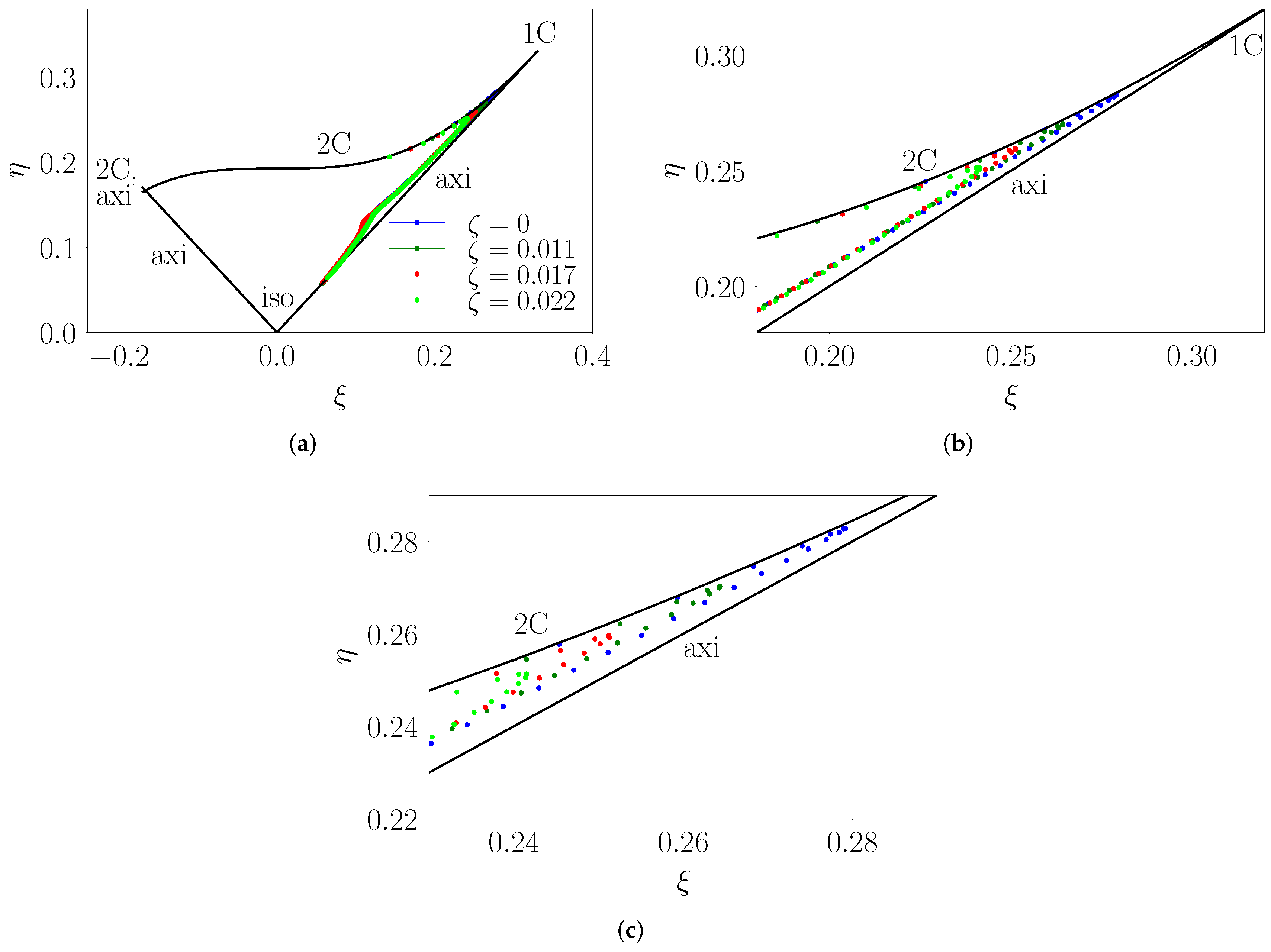
corresponding to fully isotropic Reynolds stress tensor (RS). It is well known that in turbulent boundary layers over flat topology, closer to the surface, the RS is dominated by the streamwise variance (1C) that becomes increasingly axisymmetric first and subsequently, more isotropic as one moves further away from the surface.
Figure 17 illustrates this trend clearly through the blue data points for
. As
increases, we see more of a 2C flow near the surface (as against 1C) that transitions to states with a mix of axisymmetric and isotropic nature away from the surface. This transition towards isotropic RS structure is more rapid at higher values of
bolstering the claim made in
Section 3.6.2. These trends are further confirmed by
Figure 18, which shows the diagonal elements of pressure–rate-of-strain term (
) in the variance transport. Both in the viscous and inertial layer,
,
, and
are observed to be more pronounced in magnitude for higher
, further confirming the tendency to approach isotropy faster with higher
.
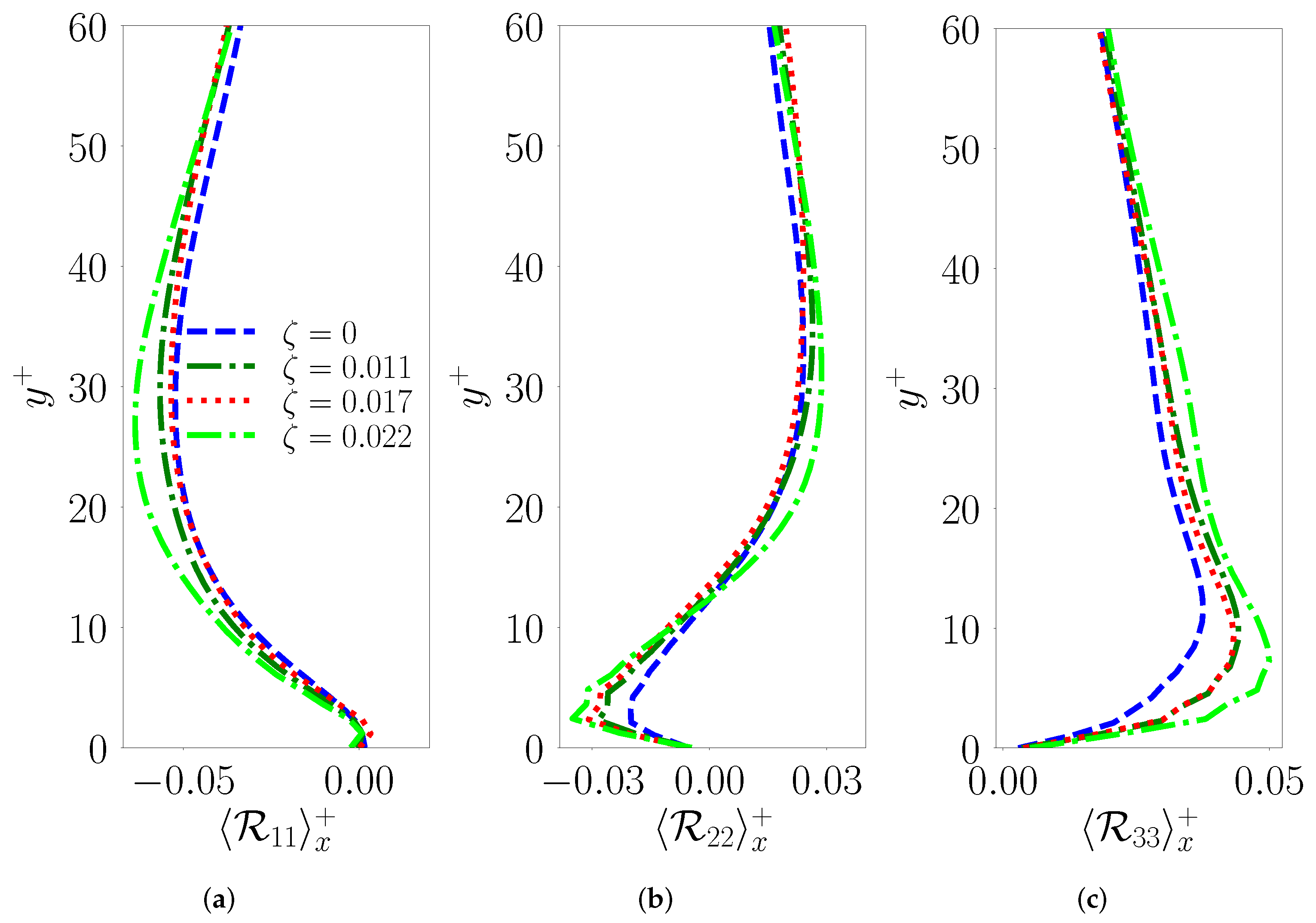
3.6.6. Vertical Turbulent Momentum Flux
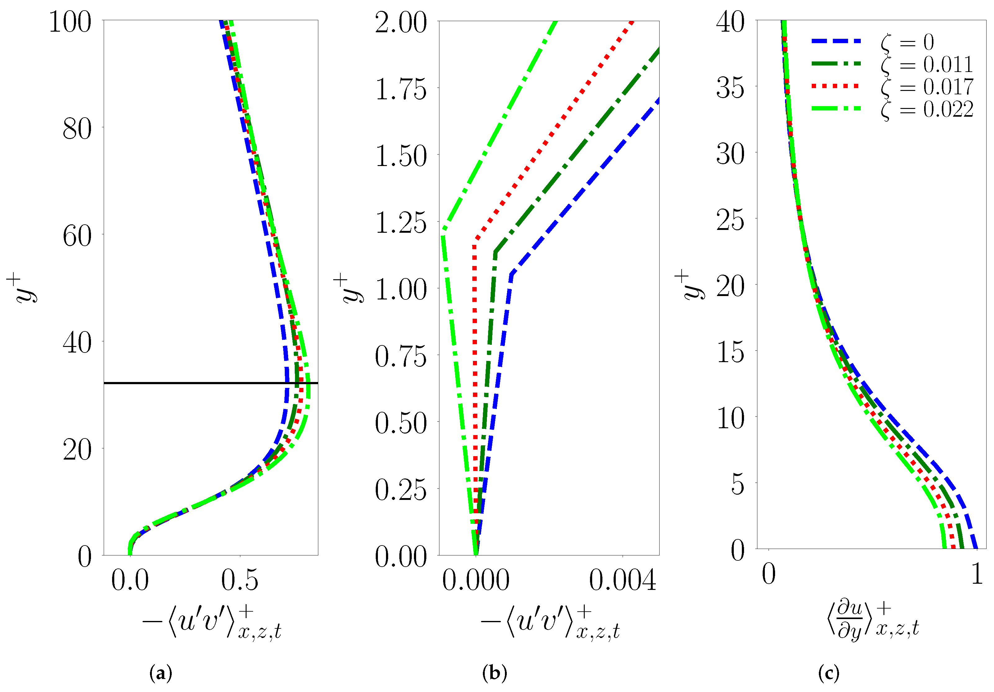
In addition to the diagonal components of the Reynolds stress tensor discussed above, we also look at the dominant off-diagonal terms, namely,
and
as shown in
Figure 14. In the limit of high Reynolds number (i.e,
), for channel flow turbulence over smooth flat surfaces, there exists a well-defined log layer with nearly constant
[
46]. This nearly constant
layer is very narrow at low Reynolds numbers. Nevertheless, this study still lets us characterize the influence of the wavelike undulation on the turbulence structure. As discussed earlier, the location of the peak in
(at
) shows very little variation with no clear trend, but its magnitude increases with
. The peak location in
falls roughly between the peak values of
and
, as shown in
Figure 13a and
Figure 15a. This increase in peak value is not surprising as the wavy surfaces naturally generate (
Figure 13b and
Figure 15b) stronger
and
fluctuations. As shown in
Figure 14a,b, increase in the positive peak of
is correlated with a small negative peak in the viscous layer at higher values of
, indicative of the surface shape induced mixing that is different from turbulence induced stress. This negative value of
close to the surface indicate that higher momentum fluid particles move away from the wall due to up slope part of the wavy surface.
4. Conclusions
In this work, we report outcomes from a DNS-based investigation of the turbulence structure and its deviation from equilibrium using turbulent boundary layer flow with modest scale separation between two infinitely parallel plates with 2D wavy undulations. In particular, we set out to assess the influence of small wave slopes (with very little flow separation) on the turbulence structure and their correspondence to common roughness characterization that invariably deals with the high slope regime. To maximize the shape sensitivity on the flow structure, we operate in a transitional roughness Reynolds number (), which is much smaller than the fully rough regime corresponding to ().
The streamwise mean velocity structure indicates a characteristic downward shift (to higher ) of the logarithmic region of the TBL, indicating increased flow drag with increase in wave slope, . This is associated with a sustained upward vertical flow in the lower roughness sublayer and corresponding downward flow in the buffer layer. The strength of these vertical motions increases with and have a dominant role to play in the near surface turbulence production processes. In fact, analysis of the mean nondimensional streamwise velocity gradients and inner-scaled turbulence production show that the buffer layer expands with increasing wave slope, , indicating that the well-known equilibrium understanding of near-wall turbulence processes is modulated even for such highly shallow wavy surfaces.
In fact, characterization of the roughness effects from such shallow surface undulations with minimal flow separation is very different from the separation and form drag dominated Nikuradse-type sand grain rough surfaces. Therefore, in our case, drag as represented by the roughness function turns out to be very weakly dependent on the wave amplitude (related to roughness height,
) and more on the effective wave slope (
). These conclusions are consistent with works by the authors of [
12,
17], where wavy surfaces in the high slope limit approach Nikuradse type roughness. Therefore, in such cases, one needs to model
as
.
In the absence of flow separation, the turbulence generation process within the roughness sublayer is primarily topology driven. For the two-dimensional surface undulations considered in this work, the differences in turbulence generation for different originate in the production of small quantities of vertical velocity variance closer to the surface due to non-zero values for the vertical velocity gradients. In contrast, for the equilibrium TBL over a flat surface, horizontal homogeneity implies that the mean vertical velocity and its gradients are zero. However, the predominant generation of vertical variance still occurs through redistribution of the streamwise velocity variance (generated closer to the surface) through the return to isotropy term. Therefore, these two different production mechanisms interact to cause to peak at a larger value and closer to the surface (relative to a flat TBL) with increasing wave steepness, ; similar trends are observed for the inner-scaled spanwise velocity variance.
The effect on the streamwise velocity variance, is more complicated. Specifically, the inner-scaled streamwise variance, (and consequently, ) displays a distinct upward shift in the location of this peak value for increasing wave steepness. In addition, the normalized peak variance magnitude decreases with . Our analysis shows that even though surface-driven changes impact the various production terms ( and ) for , the overall variance production, , does not show an upward shift in the peak. Therefore, plausible mechanisms for generation of this upward shift still point to the vertical variance being modulated through the pressure–strain term.
Overall, in the absence of significant flow separation, the surface undulations seem to generate vertical turbulence fluctuations closer to the surface which in turn modulates the entire near-wall turbulence structure. In the presence of steeper 2D waves with significant flow separation or three-dimensional wavy surfaces, the complexity will be enhanced due to the generation of spanwise fluctuations near the surface.


