Impact of Longitudinal Acceleration and Deceleration on Bluff Body Wakes

Abstract
1. Introduction
2. Numerical Setup
2.1. Numerical Grid
2.2. Model Validation
3. Results and Discussion
3.1. Body Forces
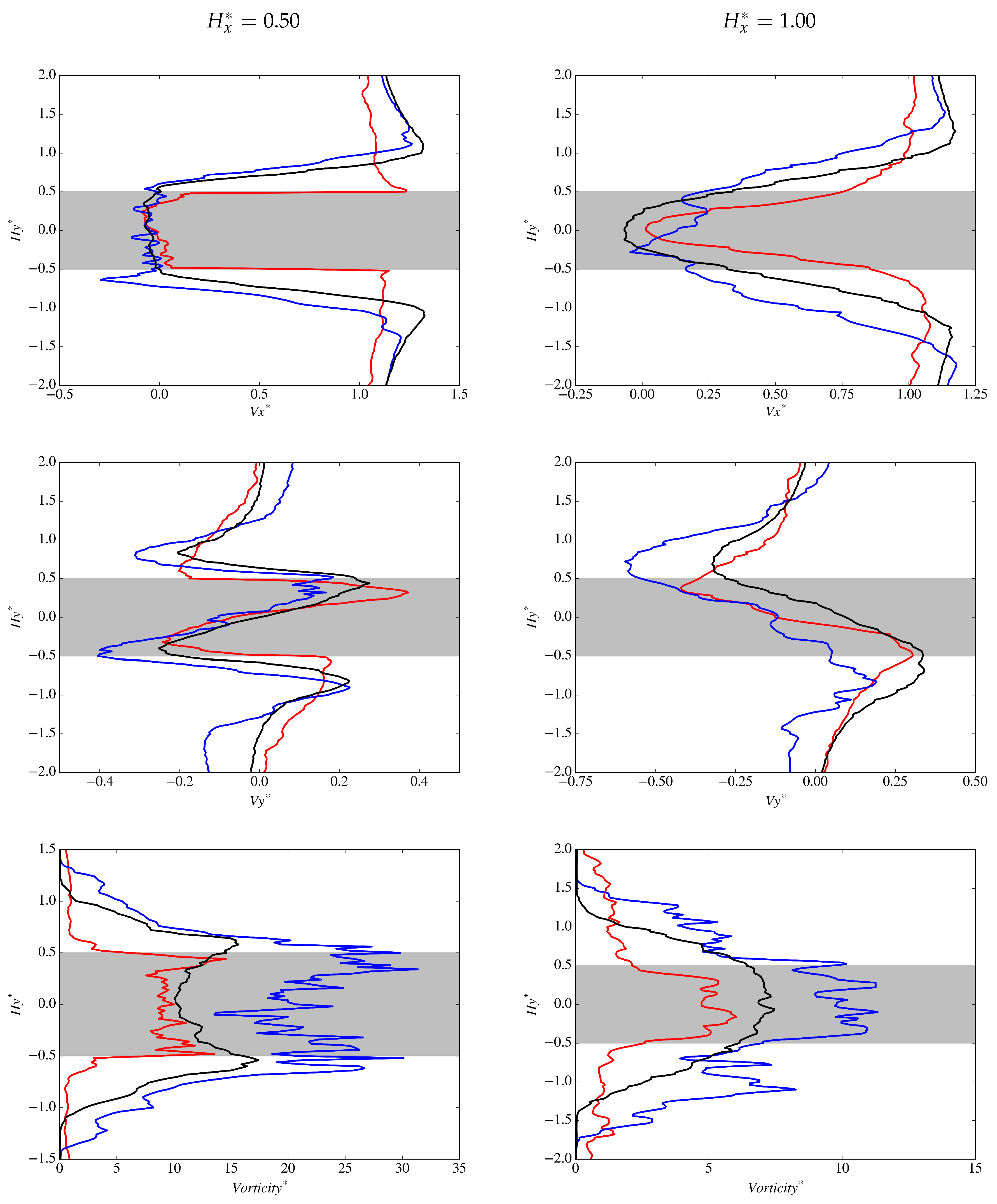
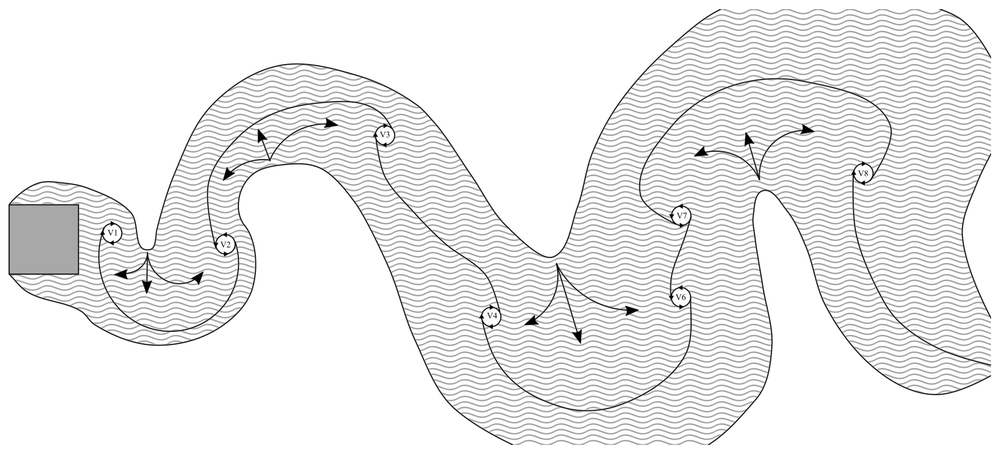
3.2. Wake Structure
4. Conclusions
Author Contributions
Funding
Acknowledgments
Conflicts of Interest
References
- Panton, R.L. Incompressible Flow, 3rd ed.; John Wiley and Sons Inc.: Hoboken, NJ, USA, 2005. [Google Scholar]
- Mohrfeld-Halterman, J.; Uddin, M. High fidelity quasi steady-state aerodynamic model effects on race vehicle performance predictions using multi-body simulation. Veh. Syst. Dyn. 2016, 54, 963–981. [Google Scholar] [CrossRef]
- Buat, P.L.G.D. Principles D’hydraulique; F. Didot: Paris, France, 1786. [Google Scholar]
- Stokes, G.G. On the Effect of the Internal Friction of Fluids on the Motion of Pendulums. Trans. Camb. Philos. Soc. 1850, IX, 8. [Google Scholar]
- Morison, J. The Force Distribution Exerted by Surface Waves on Piles; Technical Report; California University Berkeley Wave Research Lab: Berkeley, CA, USA, 1953. [Google Scholar]
- Fackrell, S.A. Study of the Added Mass of Cylinders and Spheres. Ph.D. Thesis, University of Windsor, Windsor, ON, Canada, 2011. [Google Scholar]
- Fernando, J.N.; Marzanek, M.; Bond, C.; Rival, D.E. On the separation mechanics of accelerating spheres. Phys. Fluids 2017, 29, 037102. [Google Scholar] [CrossRef]
- Lee, Y.; Rho, J.; Kim, K.H.; Lee, D.H. Fundamental studies on free stream acceleration effects on drag force in bluff bodies. J. Mech. Sci. Technol. 2011, 25, 695–701. [Google Scholar] [CrossRef]
- Roohani, H. Aerodynamic Effects of Accelerating Object in Air. Ph.D. Thesis, University of the Witwatersand, Johannesburg, South Africa, 2010. [Google Scholar]
- Zhang, Q.; Johari, H. Effects of acceleration on turbulent jets. Phys. Fluids 1996, 8, 2185–2195. [Google Scholar] [CrossRef]
- Bearman, P.; Obasaju, E. A Study of Forces, Circulation and Vortex Patterns around A Circular-Cylinder in Oscillating Flow. J. Fluid Mech. 1988, 119, 297–321. [Google Scholar] [CrossRef]
- Konstantinidis, E.; Balabani, S.; Yianneskis, M. The effect of flow perturbations on the near wake characteristics of a circular cylinder. J. Fluids Struct. 2003, 18, 367–386. [Google Scholar] [CrossRef]
- Konstantinidis, E.; Balabani, S. Flow structure in the locked-on wake of a circular cylinder in pulsating flow: Effect of forcing amplitude. Int. J. Heat Fluid Flow 2008, 29, 1567–1576. [Google Scholar] [CrossRef]
- Konstantinidis, E.; Bouris, D. Effect of nonharmonic forcing on bluff-body vortex dynamics. Phys. Rev. E 2009, 79, 045303. [Google Scholar] [CrossRef]
- Konstantinidis, E.; Liang, C. Dynamic response of a turbulent cylinder wake to sinusoidal inflow perturbations across the vortex lock-on range. Phys. Fluids 2011, 23, 075102. [Google Scholar] [CrossRef]
- Konstantinidis, E.; Bouris, D. Vortex synchronization in the cylinder wake due to harmonic and non-harmonic perturbations. J. Fluid Mech. 2016, 804, 248–277. [Google Scholar] [CrossRef]
- Peters, B. On Accelerating Road Vehicle Aerodynamics. Ph.D. Thesis, The University of North Carolina at Charlotte, Charlotte, NC, USA, 2018. [Google Scholar]
- Gritskevich, M.S.; Garbaruk, A.V.; Schütze, J.; Menter, F.R. Development of DDES and IDDES Formulations for the k-ω Shear Stress Transport Model. Flow Turbul. Combust. 2012, 88, 431–449. [Google Scholar] [CrossRef]
- Shur, M.; Spalart, P.; Travin, A. A hybrid RANS-LES approach with delayed-DES and wall-modelled LES capabilities. Int. J. Heat Fluid Flow 2008, 29, 1638–1649. [Google Scholar] [CrossRef]
- Menter, F. Two-equation eddy-viscosity modeling for engineering applications. AIAA J. 1994, 32, 1598–1605. [Google Scholar] [CrossRef]
- Han, Y.; Ding, G.; He, Y.; Wu, J.; Le, J. Assessment of the IDDES method acting as wall-modeled LES in the simulation of spatially developing supersonic flat plate boundary layers. Eng. Appl. Comput. Fluid Mech. 2017, 12, 89–103. [Google Scholar] [CrossRef]
- Trias, F.X.; Gorobets, A.; Olivia, A. Turbulent flow around a square cylinder at Reynolds number 22000: A DNS study. Comput. Fluids 2015, 123, 87–98. [Google Scholar] [CrossRef]
- Rodi, W. Comparison of LES and RANS calculations of the flow around bluff bodies. J. Wind Eng. Ind. Aerodyn. 1997, 69, 55–75. [Google Scholar] [CrossRef]
- Sohankar, A.; Davidson, L.; Norberg, C. Large eddy simulation of flow past a square cylinder: Comparison of different subgrid scale models. J. Fluids Eng. 2000, 122, 39–47. [Google Scholar] [CrossRef]
- Rodi, W.; Ferziger, J.H.; Breuer, M.; Pourquie, M. Status of large eddy simulation: Results of a workshop. J. Fluids Eng. Trans. ASME 1997, 119, 248–262. [Google Scholar] [CrossRef]
- Wong, J.; Mohebbian, A.; Kriegseis, J.; Rival, D. Rapid flow separation for transient inflow conditions versus accelerating bodies: An investigation into their equivalency. J. Fluids Struct. 2013, 40, 257–268. [Google Scholar] [CrossRef]
- Savitzky, A.; Golay, M. Smoothing and Differentiation of Data by Simplified Least Squares Procedures. Anal. Chem. 1964, 36, 1627–1639. [Google Scholar] [CrossRef]
- Jarrin, N.; Benhamadouche, S.; Laurence, D.; Prosser, R. A synthetic-eddy-method for generating inflow conditions for large-eddy simulations. Int. J. Heat Fluid Flow 2006, 27, 585–593. [Google Scholar] [CrossRef]
- Tennekes, H.; Lumley, J.L. A First Course in Turbulence; MIT Press: Cambridge, MA, USA, 1972. [Google Scholar]
- Celik, I.; Klein, M.; Freitag, M.; Janicka, J. Assessment measures for URANS/DES/LES: An overview with applications. J. Turbul. 2006, 7, N48. [Google Scholar] [CrossRef]
- Gant, S. Quality and Reliability Issues with Large-Eddy Simulation; Report RR656; Health and Safety Executive: Bootle, UK, 2008. [Google Scholar]
- Kuczaj, A.; Komen, E.; Loginov, M. Large-Eddy Simulation study of turbulent mixing in a T-junction. Nucl. Eng. Des. 2010, 240, 2116–2122. [Google Scholar] [CrossRef]
- Wilcox, D.C. Turbulence Modeling for CFD, 3rd ed.; DCW Industries Inc.: La Canada, CA, USA, 2006. [Google Scholar]
- Lyn, D.A.; Rodi, W. The flapping shear layer formed by flow separation from the forward corner of a square cylinder. J. Fluid Mech. 1994, 267, 353–376. [Google Scholar] [CrossRef]
- Cao, Y.; Tamura, T. Large-eddy simulations of flow past a square cylinder using structured and unstructured grids. Comput. Fluids 2016, 137, 36–54. [Google Scholar] [CrossRef]
- Lee, B. Some effects of turbulence scale on the mean forces on a bluff body. J. Wind Eng. Ind. Aerodyn. 1975, 1, 361–370. [Google Scholar] [CrossRef]
- Nishimura, H. Fundamental Study of Bluff Body Aerodynamics. Ph.D. Thesis, Kyoto University, Kyoto, Japan, 2001. [Google Scholar]
- Lyn, D.A.; Einav, S.; Rodi, W.; Park, J.H. A Laser-Doppler Velocimetry Study of the Ensemble-Averaged Characteristics of the Turbulent Near Wake of a Square Cylinder. J. Fluid Mech. 1995, 304, 285–319. [Google Scholar] [CrossRef]
- Cantwell, B.; Coles, D. An experimental study of entrainment and transport in the turbulent near wake of a circular cylinder. J. Fluid Mech. 1983, 136, 321–374. [Google Scholar] [CrossRef]
- Morton, B. The generation and decay of vorticity. Geophys. Astrophys. Fluid Dyn. 1984, 28, 277–308. [Google Scholar] [CrossRef]
- Griffin, O.M.; Ramberg, S.E. The vortex-street wakes of vibrating cylinders. J. Fluid Mech. 1974, 66, 553–576. [Google Scholar] [CrossRef]
- Bloor, M.S. The transition to turbulence in the wake of a circular cylinder. J. Fluid Mech. 1964, 19, 290–304. [Google Scholar] [CrossRef]
- Gerrard, J.H. The mechanics of the formation region of vortices behind bluff bodies. J. Fluid Mech. 1966, 25, 401–413. [Google Scholar] [CrossRef]


| Mesh Region | A | B | C | D | E | F |
|---|---|---|---|---|---|---|
| Grid Spacing |
| Drag (N) | |||
|---|---|---|---|
| 37.5 | 1.95 | 1.91 | |
| 0 | 71.4 | 1.33 | - |
| 102.9 | 0.52 | 1.77 |
© 2019 by the authors. Licensee MDPI, Basel, Switzerland. This article is an open access article distributed under the terms and conditions of the Creative Commons Attribution (CC BY) license (http://creativecommons.org/licenses/by/4.0/).
Share and Cite
Peters, B.; Uddin, M. Impact of Longitudinal Acceleration and Deceleration on Bluff Body Wakes. Fluids 2019, 4, 158. https://doi.org/10.3390/fluids4030158
Peters B, Uddin M. Impact of Longitudinal Acceleration and Deceleration on Bluff Body Wakes. Fluids. 2019; 4(3):158. https://doi.org/10.3390/fluids4030158
Chicago/Turabian StylePeters, Brett, and Mesbah Uddin. 2019. "Impact of Longitudinal Acceleration and Deceleration on Bluff Body Wakes" Fluids 4, no. 3: 158. https://doi.org/10.3390/fluids4030158
APA StylePeters, B., & Uddin, M. (2019). Impact of Longitudinal Acceleration and Deceleration on Bluff Body Wakes. Fluids, 4(3), 158. https://doi.org/10.3390/fluids4030158