Temperature Error Reduction of DPD Fluid by Using Partitioned Runge-Kutta Time Integration Scheme

Abstract

This study puts emphasis on reducing the temperature error of dissipative particle dynamics (DPD) fluid by directly applying a minimal-stage third-order partitioned Runge-Kutta (PRK3) method to the time integration, which does not include any of additional governing equations and change in the DPD thermostat formulation. The error is estimated based on the average values of both kinetic and configurational temperatures. The result shows that the errors in both temperatures errors are greatly reduced by using the PRK3 scheme as comparing them to those of previous studies. Additionally, the comparison among three different PRK3 schemes demonstrates our recent findings that the symplecticity conservation of the system is important to reduce the temperature error of DPD fluid especially for large time increments. The computational efficiencies are also estimated for the PRK3 scheme as well as the existing ones. It was found from the estimation that the simulation using the PRK3 scheme is more than twice as efficient as those using the existing ones. Finally, the roles of both kinetic and configurational temperatures as error indicators are discussed by comparing them to the velocity autocorrelation function and the radial distribution function. It was found that the errors of these temperatures involve different characteristics, and thus both temperatures should be taken into account to comprehensively evaluate the numerical error of DPD.

1. Introduction

The importance of mesoscopic fluid simulations has been increasing to further investigate complex phenomena at this scale with minimal computational load. At this scale (approximately ranging between 10 nm and 10 $\mathsf{\mu }$m), both hydrodynamics and thermal fluctuations are important, and thus a mesoscopic simulation method should be able to take into account these properties. Dissipative particle dynamics (DPD), which is a particle-based method first developed by Hoogerbrugge and Koleman [1], owns these properties and has been used for various simulations of mesoscopic complex fluid systems, such as colloidal suspensions [2,3], biological systems [4,5], and polymer solutions [6,7].

The reduction of the computational error of DPD is substantially important to further extend its applications, where the error is generally scaled based on the temperature of a DPD fluid system. There are three types of inter-particle forces in DPD, which are conservative, dissipative, and stochastic forces. The conservative force is derived from a potential energy function which is proportional only to inter-particle distance while the dissipative and stochastic forces play a role as a pairwise thermostat, where the dissipative force is in proportion to both inter-particle distance and relative velocity and the stochastic force involves a random noise term. A number of recent researches have mainly focused on correctly handling the dissipative force to reduce the error by modifying time integration scheme such as the modified velocity-Verlet (M-Verlet) scheme [8], the scheme using the splitting technique [9] (Shardlow scheme), and others [10,11,12,13], as well as by developing new thermostating force models including Lowe-Andersen thermostat [14] and PAdL thermostat [15]. The error reduction by the latter approach is currently outstanding [15,16]. Moreover, the effects of DPD parameters and boundary conditions on computational errors for different thermostats were studied in detail [17,18,19] more than those caused by different time integration schemes. Whereas, there are disadvantages of using these new thermostats: e.g., additional governing equations have to be taken into account, which makes it difficult to combine them with the existing DPD applications and also makes the time integration more complicating.

Reducing the temperature error via modifying time integration scheme is also challenging. There are several DPD time integration scheme in addition to the M-Verlet scheme, including Shardlow scheme [9], combining the splitting technique and Bruenger-Brooks-Karplus (BBK) method to improve the time integrations of the conservative and non-conservative parts, and the DPD-DE scheme [12], which is based on their modification of the Störmer-Verlet integration (G-JF scheme [20]), where these studies mainly focus on how to deal with the time integration of the dissipative and stochastic forces.

The straight forward way to reduce the computational error via time integration scheme is improving the order of numerical accuracy. The study of the Langevin dynamics by Abdulle et al. [21] shows that, when the time integration is split into two parts, the usual Hamiltonian part and the dissipative/stochastic part, the computational accuracy depends only on the accuracy of the Hamiltonian part, and they also found that the integration of the Hamiltonian part is not needed to be symplectic although the configurational properties become poor. These ideas have been used for the time integration of DPD [16,22]. Meanwhile, this splitting approach requires computational load to be heavier as the accuracy of the Hamiltonian part becomes higher, which can be seen in our recent study [13]. This seems to be one of the major reasons why the M-Verlet scheme has been most popularly used in DPD simulations. However, the M-Verlet scheme can cause a large error at large time increments which could become more than 5% in temperature corresponding to the deviation more than 10${}^{\circ }$ K.

Recent studies [13,16] show that the M-Verlet scheme gives almost the same error (measured by temperature error) to that of the splitting scheme by Shardlow [9]. On the other hand, in our recent study, the Shardlow scheme was modified by replacing the velocity-Verlet scheme to a high-order symplectic integration scheme for the integration of the Hamiltonian part (so-called modified Shardlow (M-Shardlow) scheme). The error was estimated based on the configurational temperature [23], and the results by using the M-Shardlow scheme showed that the temperature error was reduced to the similar extent to that by using the current high-performance thermostat [15] at the time increments which are often employed for DPD simulations. These facts indicate that it seems to be possible to reduce the error by directly apply higher symplectic time integration schemes to DPD without treating the time integration of dissipative and stochastic forces, though this approach does not improve the order of time integration accuracy. This is the motivation of the present study.

The time integration scheme utilizing the Partitioned Runge-Kutta (PRK) method (the PRK scheme) is recognized as a symplectic scheme developed for Hamiltonian systems, and, especially, the third-order PRK (PRK3) scheme developed by Ruth [24] is well known because it requires only minimal stages to obtain the targeted order of accuracy while keeping the symplecticity conservation. This characteristics is significantly advantageous to attain both error and computational cost reductions without any of additional governing equations and change in the DPD thermostat model. Therefore, in the present study, it is motivated that the PRK3 scheme is directly applied for the DPD time integration, and the temperature error obtained by using this scheme is compared with those by the existing schemes to evaluate the efficiency of this scheme for reducing the error. Also, there exists three different solutions for the coefficient equations of the PRK3 scheme proposed by Ruth [24] and Iwatsu [25] to date, and effect of these coefficients on the DPD error is investigated in this study.

Another major motivation of this study is to investigate what the errors in kinetic and configurational temperatures involve in detail. Most of early DPD researches mainly considered that the kinetic temperature is the representative to be evaluated for the DPD error, which is calculated from system kinetic energy, i.e., only particle momenta are taken into account. Recent studies [26,27], on the other hand, estimated the system temperature with a different fashion using only particles’ configurational information and found that error in this temperature is larger than the kinetic one. This temperature is usually called the configurational temperature [23] which has become another indicator to scale the DPD error, which is sometimes referred to as more important value than the kinetic temperature. Although most of current studies [13,15,16] estimate the errors in both temperatures, the roles of kinetic and configurational temperatures as error indicators are still unclear. This is one of the motivations for the present study to investigate what is reflected through estimating the kinetic and configurational temperature errors in detail.

This paper is organized as follows. The numerical methods and time integration schemes are described in detail in the next section. In Section 3, the comparisons of the results between the PRK3 schemes and the existing schemes, including the M-Verlet [8], Shardlow [9], and M-Shardlow schemes [13] are firstly made via both kinetic and configurational temperatures. Secondly, the radial distribution function and velocity autocorrelation function are calculated to evaluate the reductions in these errors by using the PRK3 schemes. The roles of kinetic and configurational temperatures as error indicators are also investigated by comparing the relative errors of those quantities and the temperatures. In addition, the computational efficiency of the PRK3 scheme is compared to those of the existing schemes. Finally, in Section 4, the results obtained in this study are summarized.

2. Methodology

2.1. Governing Equations

In the DPD method, each DPD particle is considered to represent a cluster of actual molecules of the flow field and it moves in Lagrangian fashion. Each particle interacts with surrounding particles through the conservative, dissipative, and stochastic forces within a certain cutoff radius, $r_c$. For readers’ convenience, the DPD equations of motion [28] for ith particle are expressed as follows based on our previous paper [13]:

$$\begin{array}{c}\hfill \mathrm{d}\left[\begin{array}{c}\hfill {\mathbf{q}}_{\mathit{i}}\\ \hfill {\mathbf{p}}_{\mathit{i}}\end{array}\right]=\left[\begin{array}{c}{\mathbf{p}}_{\mathit{i}}/{\mathit{m}}_{\mathit{i}}\\ {\mathbf{F}}_{\mathit{i}}^{\mathbf{C}}+{\mathbf{F}}_{\mathit{i}}^{\mathbf{D}}+{\mathbf{F}}_{\mathit{i}}^{\mathbf{R}}\end{array}\right]\mathrm{d}\mathit{t},\end{array}$$

(1)

where ${\mathbf{F}}_{\mathit{i}}^{\mathbf{C}}$, ${\mathbf{F}}_{\mathit{i}}^{\mathbf{D}}$, and ${\mathbf{F}}_{\mathit{i}}^{\mathbf{R}}$ are the conservative, dissipative, and stochastic forces, respectively. The following soft potential function was originally adopted for the DPD simulation [28].

$$U\left(r_{ij}\right)=\left\{\begin{array}{cc}\hfill \sum _{\mathit{j}\ne \mathit{i}}\frac{a_{ij}{r}_c}{2}{\left(1-\frac{r_{ij}}{r_c}\right)}^2& \hfill :\hspace{1em}(r_{ij}<r_c),\\ 0& \hfill :\hspace{1em}(r_{ij}\ge r_c).\end{array}\right.$$

(2)

In the above equation, the parameter $a_{ij}$ is the maximum repulsion between the particles. This potential results in the following form of conservative force.

$$\begin{array}{c}\hfill {\mathbf{F}}_{\mathit{i}}^{\mathbf{C}}=\left\{\begin{array}{cc}\hfill \sum _{\mathit{j}\ne \mathit{i}}{\mathit{a}}_{\mathit{ij}}\left(1-\frac{{\mathit{r}}_{\mathit{ij}}}{{\mathit{r}}_{\mathit{c}}}\right){\mathbf{e}}_{\mathit{ij}}& \hfill :\hspace{1em}({\mathbf{r}}_{\mathbf{ij}}<{\mathbf{r}}_{\mathbf{c}}),\\ 0& \hfill :\hspace{1em}({\mathbf{r}}_{\mathbf{ij}}\ge {\mathbf{r}}_{\mathbf{c}}).\end{array}\right.\end{array}$$

(3)

Also, the dissipative and stochastic forces are described by:

$$\begin{array}{ccc}\hfill {{\mathbf{F}}^{\mathbf{D}}}_{\mathit{i}}& =& -\sum _{\mathit{j}\ne \mathit{i}}{\gamma }_{\mathit{ij}}{\omega }^D\left(r_{ij}\right)\left({\mathbf{e}}_{\mathit{ij}}·{\mathbf{v}}_{\mathit{ij}}\right){\mathbf{e}}_{\mathit{ij}},\hfill \end{array}$$

(4)

$$\begin{array}{ccc}\hfill {\mathbf{F}}_{\mathit{i}}^{\mathbf{R}}& =& \sum _{\mathit{j}\ne \mathit{i}}{\sigma }_{ij}{\omega }^R\left(r_{\mathit{ij}}\right){\zeta }_{\mathit{ij}}\mathrm{d}{\mathit{t}}^{-1/2}{\mathbf{e}}_{\mathit{ij}}.\hfill \end{array}$$

(5)

In Equations (3)–(5), the vector ${\mathbf{r}}_{ij}$ points i to j such that ${\mathbf{r}}_{ij}={\mathbf{q}}_i-{\mathbf{q}}_j$ and ${\mathbf{v}}_{\mathit{ij}}={\mathbf{v}}_i-{\mathbf{v}}_j$. The vecotr ${\mathbf{e}}_{\mathit{ij}}$ is the unit vector pointing in the direction from i to j, i.e., ${\mathbf{e}}_{\mathit{ij}}={\mathbf{r}}_{\mathit{ij}}/\left|{\mathbf{r}}_{\mathit{ij}}\right|$. Parameters ${\gamma }_{ij}$ and ${\sigma }_{ij}$ are the strength of dissipative and stochastic forces, respectively. ${\zeta }_{ij}$ is a random number with zero mean and unit variance (Gausisian white noise), and ${\zeta }_{ij}={\zeta }_{ji}$ is satisfied to conserve the momentum of the interacting pair of particles. ${\omega }^D\left(r_{ij}\right)$ and ${\omega }^R\left(r_{ij}\right)$ are the weight functions for the dissipative and stochastic forces, respectively. A general form of ${\omega }^D\left(r_{ij}\right)$ is given by [29]:

$${\omega }^D\left(r_{ij}\right)=\left\{\begin{array}{cc}\hfill {\left(1-\frac{r_{ij}}{r_c}\right)}^{n_e}& \hfill :\hspace{1em}(r_{ij}<r_c),\\ 0& \hfill :\hspace{1em}(r_{ij}\ge r_c),\end{array}\right.$$

(6)

where $n_e$ is the exponent that can control the viscosity of the DPD fluid. In this study, the standard value, $n_e=2$, is used [28]. Also, the following conditions have to be satisfied which are the fluctuation-dissipation relation for DPD.

$$\begin{array}{c}\hfill {\omega }^D\left(r_{ij}\right)={\omega }^R{\left(r_{ij}\right)}^2,{\gamma }_{ij}=\frac{{\sigma }_{ij}^2}{2k_{B}T},\end{array}$$

(7)

where $k_B$ and T are the Boltzmann constant and target equilibrium temperature, respectively.

2.2. Time Integration Algorithms

The discretized time evolution of the DPD system from $t_n$ to $t_{n+1}=t_n+\Delta t$ ($\Delta t$: time increment) can be described as follows:

$$\begin{array}{c}\hfill \left[\begin{array}{c}\hfill {\mathbf{q}}^{\mathrm{n}+1}\\ \hfill {\mathbf{p}}^{\mathrm{n}+1}\end{array}\right]=exp\left(\Delta t\left[{\mathcal{D}}_{{\mathcal{L}}_p}+{\mathcal{D}}_H\right]\right)\left[\begin{array}{c}\hfill {\mathbf{q}}^{\mathrm{n}}\\ \hfill {\mathbf{p}}^{\mathrm{n}}\end{array}\right],\end{array}$$

(8)

where the superscripts $\mathrm{n}$ and $\mathrm{n}+1$ denote time steps correspondent with $t_n$ and $t_{n+1}$, respectively. ${\mathcal{D}}_H$ and ${\mathcal{D}}_{{\mathcal{L}}_p}$ in Equation (8) are the operators described by the following equations defined by Español and Warren [28].

$$\begin{array}{ccc}\hfill {\mathcal{D}}_H& =& \sum _i\left[\frac{{\mathbf{p}}_i}{m_i}\frac{\partial }{\partial {\mathbf{q}}_i}+{\mathbf{F}}_i^{\mathbf{C}}\frac{\partial }{\partial {\mathbf{p}}_i}\right],\hfill \\ \hfill {\mathcal{D}}_{{\mathcal{L}}_p}& =& \sum _i\left[\sum _{j\ne i}\left\{-{\gamma }_{\mathit{ij}}{\omega }^D\left(r_{ij}\right)\left({\mathbf{e}}_{\mathit{ij}}·{\mathbf{v}}_{\mathit{ij}}\right)\right.\right.\hfill \end{array}$$

(9)

$$\begin{array}{cc}+& \left.\left.\frac{{\sigma }_{ij}^2}{2}{\left({\omega }^R\left(r_{\mathit{ij}}\right)\right)}^2\left(\frac{\partial }{\partial {\mathbf{p}}_i}-\frac{\partial }{\partial {\mathbf{p}}_j}\right)\right\}{\mathbf{e}}_{\mathit{ij}}\frac{\partial }{\partial {\mathbf{p}}_i}\right].\hfill \end{array}$$

(10)

${\mathcal{D}}_H$ described by Equation (9) is the standard Liouville operator (conservative part) widely known for Hamiltonian systems, and ${\mathcal{D}}_{{\mathcal{L}}_p}$ described by Equation (10) is equivalent to the dissipative and stochastic forces (non-conservative part). In the above equation, the term, $exp\left(\Delta t\left[{\mathcal{D}}_H+{\mathcal{D}}_{{\mathcal{L}}_p}\right]\right)$, is “phase space propagator” (PSP). There are several DPD time integration schemes by splitting this PSP with the Baker-Campbell-Hausdorff (BCH) formulation [9,13,15,16]. In this study, the simulations are performed by using partitioned Runge-Kutta (PRK) schemes and the results are compared with those by employing the modified Verlet (M-Verlet) [8], Shardlow [9], and M-Shardlow [13] schemes. The description of the PRK schemes is in the following subsection in detail while those of the other schemes are summarized in Appendix A.

Partitioned Runge-Kutta Scheme

Partitioned Runge-Kutta (PRK) scheme is a type of symplectic time integration schemes. In contrast to ordinary Runge-Kutta schemes, the PRK scheme can preserve the canonical character of Hamiltonian systems. In this study, a form of the third-order accurate PRK (PRK3) scheme developed by Ruth [24] is employed because minimal number of stages are required to obtain the third order accuracy. The algorithm of the PRK3 schemes for integration time increment $\Delta t$ is expressed as follows:

$$\begin{array}{ccc}\hfill {\mathbf{p}}_0& =& {\mathbf{p}}_i\left(t\right),{\mathbf{q}}_0={\mathbf{q}}_i\left(t\right),\hfill \\ \hfill {\mathbf{p}}_1& =& {\mathbf{p}}_0+b_1\Delta t\mathbf{F}({\mathbf{q}}_0,{\mathbf{p}}_0,t),\hfill \\ \hfill {\mathbf{q}}_1& =& {\mathbf{q}}_0+{\widehat{b}}_1\Delta t{\mathbf{p}}_1,\hfill \\ \hfill {\mathbf{p}}_2& =& {\mathbf{p}}_1+b_2\Delta t\mathbf{F}({\mathbf{q}}_1,{\mathbf{p}}_1,t+{\widehat{b}}_1\Delta t),\hfill \\ \hfill {\mathbf{q}}_2& =& {\mathbf{q}}_1+{\widehat{b}}_2\Delta t{\mathbf{p}}_2,\hfill \\ \hfill {\mathbf{p}}_3& =& {\mathbf{p}}_2+b_3\Delta t\mathbf{F}({\mathbf{q}}_2,{\mathbf{p}}_2,t+({\widehat{b}}_1+{\widehat{b}}_2)\Delta t),\hfill \\ \hfill {\mathbf{q}}_3& =& {\mathbf{q}}_2+{\widehat{b}}_3\Delta t{\mathbf{p}}_3,\hfill \end{array}$$

(11)

where $\mathbf{F}$ denotes the summation of conservative, dissipative, and stochastic forces, i.e., $\mathbf{F}={\mathbf{F}}^{\mathbf{C}}+{\mathbf{F}}^{\mathbf{D}}+{\mathbf{F}}^{\mathbf{R}}$. Also, $b_1$, $b_2$, $b_3$, ${\widehat{b}}_1$, ${\widehat{b}}_2$, and ${\widehat{b}}_3$ are coefficients which satisfy the following five conditions:

$$\begin{array}{ccc}\hfill b_1+b_2+b_3& =& 1,\hfill \end{array}$$

(12)

$$\begin{array}{ccc}\hfill b_2{\widehat{b}}_1+b_3({\widehat{b}}_1+{\widehat{b}}_2)& =& \frac{1}{2},\hfill \end{array}$$

(13)

$$\begin{array}{ccc}\hfill b_2{\widehat{b}}_1^2+b_3{({\widehat{b}}_1+{\widehat{b}}_2)}^2& =& \frac{1}{3},\hfill \end{array}$$

(14)

$$\begin{array}{ccc}\hfill {\widehat{b}}_1+{\widehat{b}}_2+{\widehat{b}}_3& =& 1,\hfill \end{array}$$

(15)

$$\begin{array}{ccc}\hfill {\widehat{b}}_1{b}_1^2+{\widehat{b}}_2{(b_1+b_2)}^2+{\widehat{b}}_3{(b_1+b_2+b_3)}^2& =& \frac{1}{3}.\hfill \end{array}$$

(16)

Three different solutions are known for the system Equations (12)–(16) found by Ruth [24] and Iwatsu [25], which we call PRK3 (Ruth), PRK3 (Iwatsu A), and PRK3 (Iwatsu B) schemes in this sutudy. The coefficients for PRK3 (Ruth), PRK3 (Iwatsu A), and PRK3 (Iwatsu B) schemes are listed in

Table 1. Coefficients of the PRK3 schemes.

	Ruth [24]	Iwatsu A [25]	Iwatsu B [25]
$b_1$	$\frac{7}{24}$	$\frac{-7+\sqrt{209/2}}{12}$	$-\frac{7+\sqrt{209/2}}{12}$
$b_2$	$\frac{3}{4}$	$\frac{11}{12}$	$\frac{11}{12}$
$b_3$	$-\frac{1}{24}$	$\frac{8-\sqrt{209/2}}{12}$	$\frac{8+\sqrt{209/2}}{12}$
${\widehat{b}}_1$	$\frac{2}{3}$	$\frac{2}{9}\left(1+\sqrt{\frac{38}{11}}\right)$	$\frac{2}{9}\left(1-\sqrt{\frac{38}{11}}\right)$
${\widehat{b}}_2$	$-\frac{2}{3}$	$\frac{2}{9}\left(1-\sqrt{\frac{38}{11}}\right)$	$\frac{2}{9}\left(1+\sqrt{\frac{38}{11}}\right)$
${\widehat{b}}_3$	1	$\frac{5}{9}$	$\frac{5}{9}$

.

3. Results and Discussion

3.1. Simulation Details

A set of simulations were implemented to compare the temperature errors estimated by using the PRK3 scheme to that by using the existing ones (M-Verlet, Shardlow, and M-Shardlow schemes), where an in-house computational code package were developed with Python and Fortran to perform these simulations. The system considered in this study is a cubic box having a length of $L=10$ with the periodic boundaries for all the directions, where $N_{tot}=4000$ of DPD particles was randomly distributed initially in the computational domain such that the number density becomes ${\rho }_{DPD}=4$. As mentioned in the introduction section, the present study is motivated to reduce the temperature error by modifying time integration scheme and to evaluate the efficiency of the PRK3 scheme by comparing it with the existing schemes. Therefore, the choice of the simulation parameters considered in the present study is followed by our previous study [13] as well as the recent relevant studies [12,15,16], i.e., $m_i=1$, $r_c=1$, $a_{ij}=18.75$, ${\gamma }_{ij}$ = 4.5, $k_{B}T=1$, and $n_e=2$, and there is no external force applied to induce flow. This set of parameters gives a Schmidt number (Sc) approximately corresponding to those of gases such as air and oxygen. This is calculated to be 0.680 as a reference by using the equation, $\mathrm{Sc}=0.5+{\left(2\pi {\gamma }_{ij}\rho r_c\right)}^2/70875k_{B}T$, introduced by Groot and Warren [8], while a recent study by Li et al. [30] shows that the Sc value can be widely controlled up to about a thousand by only changing the $n_e$ (see Equation (6)) and $k_{B}T$ values. Also, the set of random numbers ${\zeta }_{ij}$ does not change within a time step in accordance with the characteristics of the Wiener process for all the time integration schemes. The simulations were implemented for the time increments, $\Delta t$ ranging between 0.005 and 0.1, which includes those used in a number of DPD studies [5,31,32,33,34]. Also, each of them were performed at least 1000 DPD time (t).

As shown in the previous studies [9,11,12,15,16,30], the kinetic and configurational temperatures have been recently used to measure the temperature error. In this study, both temperatures are calculated to evaluate how the errors of these temperatures are connected to the reliabilities of physical properties. The kinetic and configurational temperatures is calculated using the following equations [23].

$$\begin{array}{ccc}\hfill {\left(k_{B}T\right)}_K& =& \frac{{\sum }_i({\mathbf{p}}_i^2/m_i)}{d\left(N_{tot}-1\right)},\hfill \end{array}$$

(17)

$$\begin{array}{ccc}\hfill {\left(k_{B}T\right)}_C& =& \frac{{\sum }_i^{N_{tot}}{\left|{{\mathbf{F}}^{\mathbf{C}}}_i\right|}^2}{{\sum }_i^{N_{tot}}\left(-{\nabla }_i·{{\mathbf{F}}^{\mathbf{C}}}_i\right)}.\hfill \end{array}$$

(18)

In Equation (17), $d=3$ is used in this study. The temperature errors can be estimated as follows:

$$\begin{array}{c}\hfill {ϵ}_{〈k_B{T}_l〉}=\frac{\left|k_{B}T-〈k_B{T}_l〉\right|}{k_{B}T},\end{array}$$

(19)

where the subscript, l, expresses either K or C, and $〈k_B{T}_l〉$ is the averaged temperature.

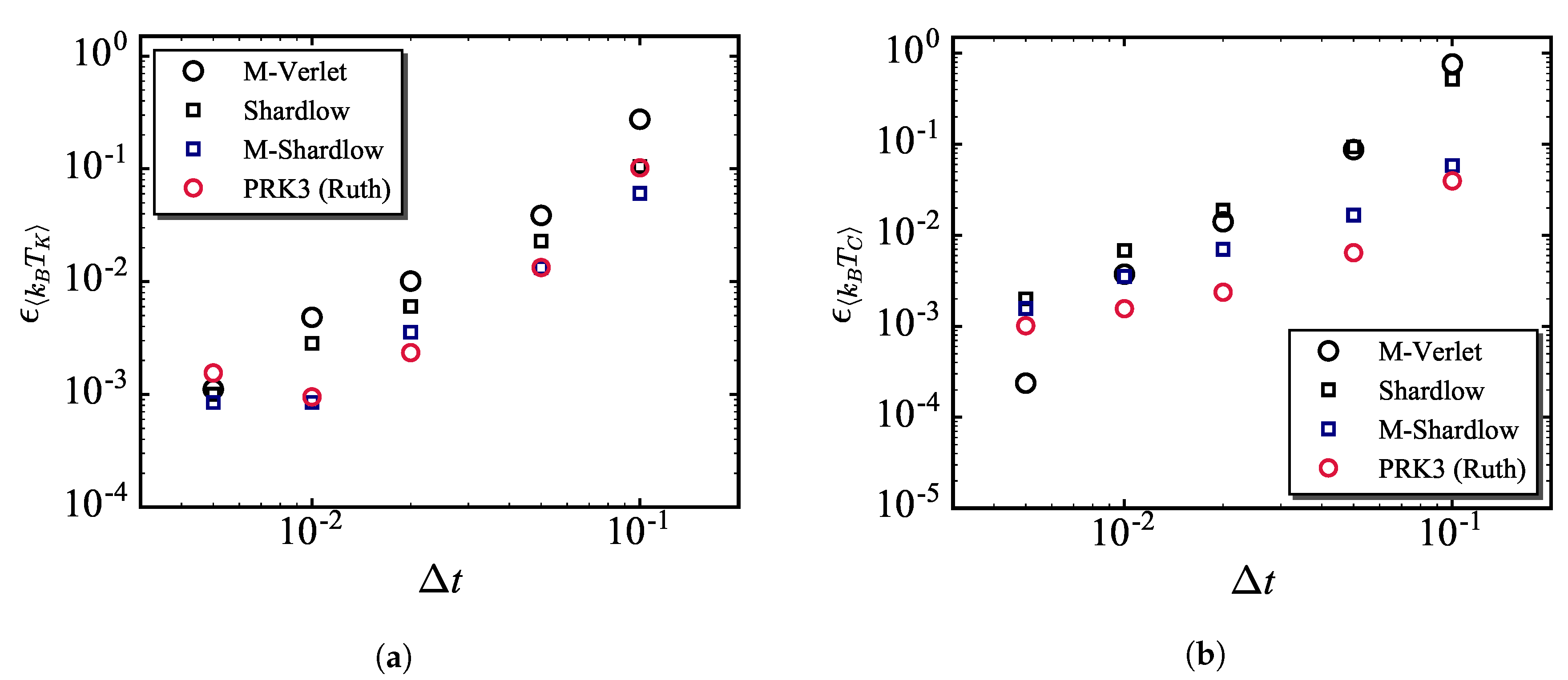
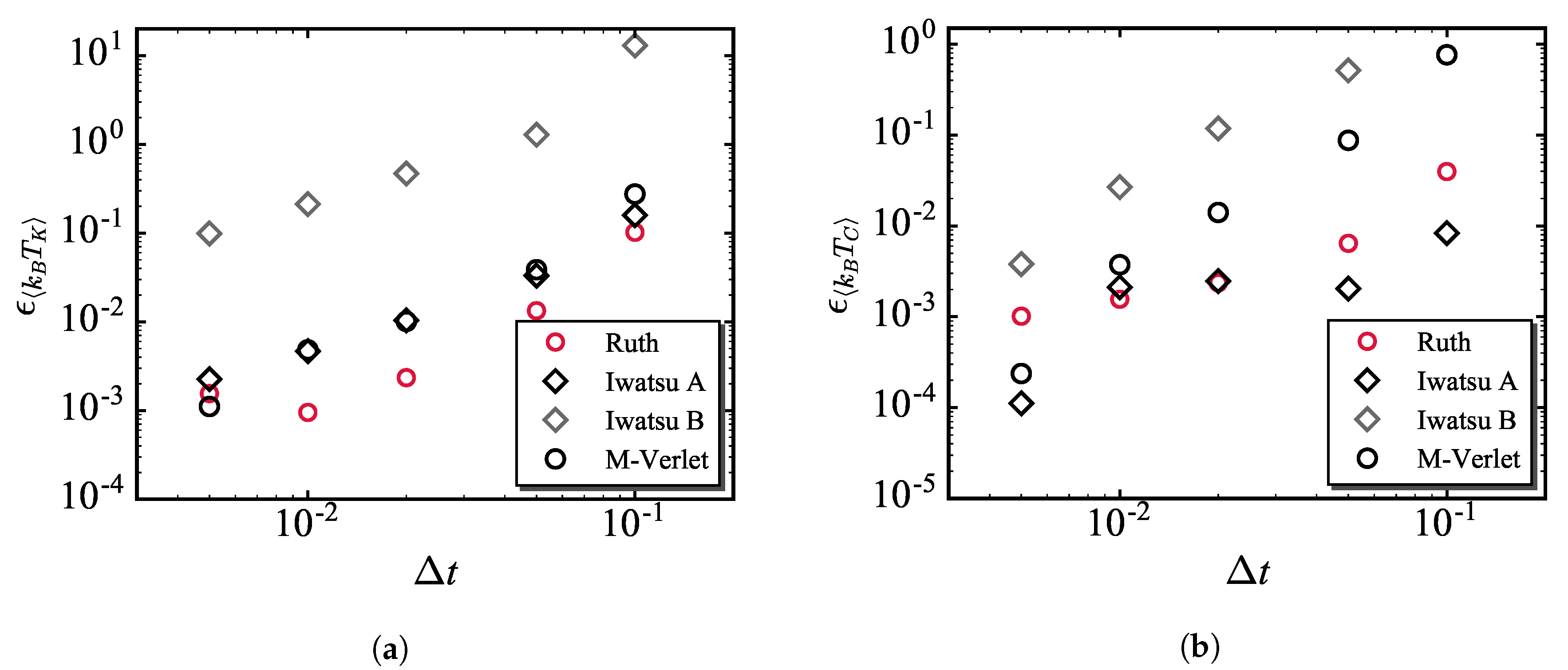
3.2. Temperature Errors on Different Time Integration Schemes

Figure 1a,b show the change in the error of averaged kinetic and configurational temperatures for different time integration schemes, respectively. First, as can be seen in Figure 1a, the error almost monotonically increases with increasing time increment regardless of time integration scheme. Comparing the results for different integration schemes, the errors of the PRK3 (Ruth) scheme and the M-Shardlow scheme are better than those of existing schemes for almost the entire $\Delta t$ range while the errors tend to coincide to each other as $\Delta t$ decreases. Next, as shown in Figure 1b, the configurational temperature errors for all the time integration schemes monotonically increase as well as the kinetic temperature errors. Also, unlike the results of the kinetic temperature error, the configurational temperature errors of the PRK3 (Ruth) scheme are better than the results of the M-Shardlow schemes. This indicates that the PRK3 (Ruth) scheme is more efficient than the M-Sharldow scheme because the number of force evaluations for the PRK3 (Ruth) scheme is smaller than that for the M-Shardlow, which will be discussed in a later section.

Figure 2a,b show the comparisons of the kinetic and configurational temperatures among the three PRK3 schemes, i.e., Ruth, Iwatsu A, and Iwatsu B. As can be seen in both figures, it is obvious that the results of the PRK3 (Iwatsu B) scheme is remarkably inferior to those of other PRK3 schemes. It can be observed that the result of the PRK3 (Iwatsu A) scheme is superior to that of the PRK3 (Ruth) scheme while the errors almost correspond to each other for $\Delta t=0.01$ and 0.02. For the kinetic temperature error, on the other hand, the performance of the PRK3 (Iwatsu A) scheme results in the same extent as the M-Verlet scheme. The results of the PRK3 (Ruth) scheme only show the improvements in both temperatures compared to the existing schemes.

The numerical study by Iwatsu [25] shows that the PRK3 (Iwatsu A) scheme is slightly more numerically reliable and less dispersive than the PRK3 (Ruth) scheme while the PRK3 (Iwatsu B) scheme is the worst in both of them among the three PRK3 schemes. The results shown in Figure 2 is almost in accordance with this outcome especially for $\Delta t>0.02$ though the time integrations of the non-conservative part for these PRK3 schemes differently influence on the temperature error as well as the conservative part. This indicates that the effect of the conservative part on the computational error is greater than that of the non-conservative part, which leads to the same conclusion in our previous study that the effect of conservative force dominates computational error larger than those of the other forces especially for large time increments [13]. This effect exists in any simulation conditions. Therefore, it is expected that the temperature error can be reduced by using the PRK3 schemes in different simulation conditions where, for example, flows are involved and/or the DPD fluids have water-like characteristics, i.e., higher Schmidt numbers.

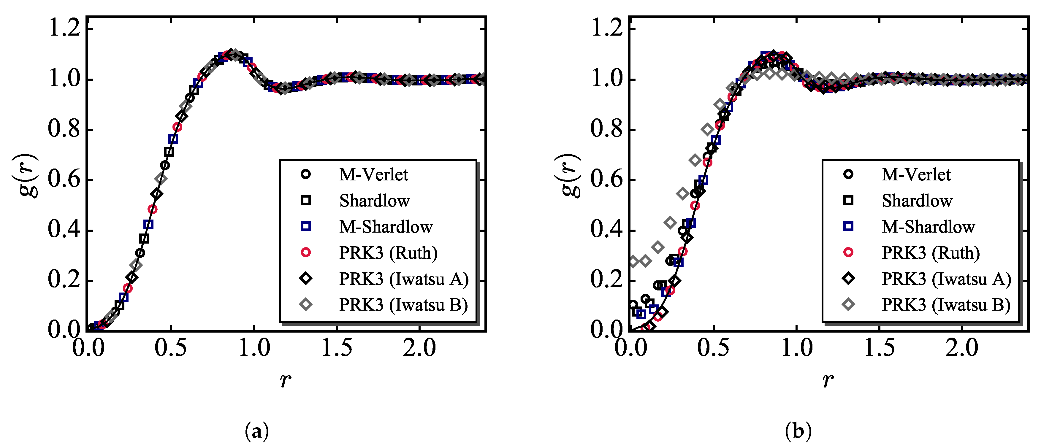
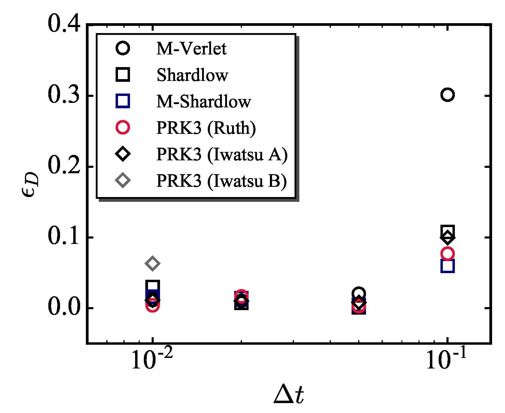
3.3. Errors in Configurational and Dynamic Properties

The computational errors of different time integration schemes in terms of configurational and dynamics properties are also investigated, where radial distribution function, $g\left(r\right)$, and velocity autocorrelation function (VACF), $C_v$, are selected as the representative configurational and dynamic quantities as were chosen in the previous studies [9,13,16]. The $g\left(r\right)$ value can be regarded as the normalized local number density at the distance, r (r: interparticle distance), which can be described in the discrete form as follows:

$$\begin{array}{c}\hfill g\left(r\right)=\frac{〈\Delta n〉}{4\pi r^2{\rho }_{DPD}\Delta r},\end{array}$$

(20)

where $〈\Delta n〉$ is the time-averaged number of DPD particles existing in the volume of $4\pi r^2\Delta r$.

Figure 3a,b show the $g\left(r\right)$ values as a function of the distance r for $\Delta t$ = 0.01 and 0.1, respectively, along with the $g\left(r\right)$ distribution of the M-Verlet scheme for $\Delta t=0.005$ as a reference. As can be seen in Figure 3a, all the $g\left(r\right)$ distributions coincide with each other regardless of time integration scheme. In the cases for $\Delta t$ = 0.1, however, it is observed that the $g\left(r\right)$ distributions in the vicinity of $r=0$ deviate from the reference distribution except for the results of the PRK3 (Ruth) and PRK3 (Iwatsu A) schemes.

In order to evaluate the $g\left(r\right)$ deviation quantitatively, the system potential energy is calculated using the following equation:

$$\begin{array}{c}\hfill 〈U〉={\int }_0^{r_c}4\pi r^{2}g\left(r\right){\rho }_{DPD}U\left(r\right)\mathrm{d}\mathit{r}.\end{array}$$

(21)

Based on the above equation, the error in this value for each time integration scheme can be estimated as follows:

$$\begin{array}{c}\hfill {ϵ}_{〈U〉}=\frac{\left|〈U〉-{〈U〉}_0\right|}{{〈U〉}_0},\end{array}$$

(22)

where ${〈U〉}_0$ is the the potential energy for $\Delta t=0.005$. Figure 4 shows the ${ϵ}_{〈U〉}$ value as a function of $\Delta t$ for different time integration schemes. It can be observed in this figure that the error is not so influenced by the time increment for $\Delta t<0.01$ for all the results. Whereas, for the larger time increments, the error becomes larger as the $\Delta t$ increases on the results of the M-Verlet, Shardlow, and PRK3 (Iwatsu B) schemes. The results of the M-Shardlow, PRK3 (Ruth), and PRK3 (Iwatsu A) schemes, on the other hand, stay at very low values for the entire time increment range. Looking into the results for $\Delta t=0.1$, the errors in potential energy are ranked in the same order of those in configurational temperature (see Figure 1b and Figure 2b). Therefore, it can be verified by this result that the configurational temperature is an indicator having the dimension of temperature to scale how configurational quantities are numerically valid.

VACF, $C_v$, is the measure of self-diffusion coefficient and is expressed as follows:

$$\begin{array}{c}\hfill C_v\left(\tau \right)=〈\overline{\mathbf{v}\left(\tau \right)·\mathbf{v}\left(\tau =0\right)}〉,\end{array}$$

(23)

where $\tau$ is the delay time. The self-diffusion coefficient can be calculated by integrating this value with respect to time, that is;

$$\begin{array}{c}\hfill D=\frac{1}{d}{\int }_0^{\infty }{C}_v\left(s\right)\mathrm{d}\mathit{s}.\end{array}$$

(24)

The discretized form of the above equation can be written as follows if the trapezoidal formula is used:

$$\begin{array}{c}\hfill D=\frac{1}{d}{\Sigma }_0^{\infty }\frac{\left[C_v\left(s+\Delta s\right)+C_v\left(s\right)\right]}{2}\Delta \mathit{s}.\end{array}$$

(25)

Therefore, similar to the error in the potential energy, the error in this value can be expressed as

$$\begin{array}{c}\hfill {ϵ}_D=\frac{\left|D-D_0\right|}{D_0},\end{array}$$

(26)

where $D_0$ is the value for $\Delta t=0.005$. In this study, the $\Delta s$ value is fixed to the maximum value, i.e., $\Delta s=0.1$, in order to eliminate this effect on the D value estimated by the simulations with different time increments.

The $C_v$ distributions as a function of the delay time, $\tau$, on different time integration schemes for $\Delta t$ = 0.005 and 0.1 are shown in Figure 5a,b, respectively. As shown in Figure 5a, all the VACF distributions are almost identical for $\Delta t$ = 0.005 while the result by using the PRK3 (Iwatsu B) already deviates from those by the other results. Also, it can be seen that the $C_v$ value almost converges to zero at $\tau =2$. Figure 5b shows, on the other hand, that the $C_v$ distributions for $\Delta t$ = 0.1 are larger than those for $\Delta t$ = 0.005, which seems to be due to the kinetic temperature error increasing as $\Delta t$ becomes larger.

The error in VACF is quantitatively evaluated using Equation (26) and Figure 6 shows the ${ϵ}_D$ value as a function of $\Delta t$, where the integration was taken up to $\tau =2$. As can be seen in this figure, the ${ϵ}_D$ value increases as $\Delta t$ increases. Also, it can be seen in the results for $\Delta t$ = 0.1 that the order of the error in kinetic temperature is almost reflected to that in the ${ϵ}_D$ value. A notable difference between ${ϵ}_{〈U〉}$ and ${ϵ}_D$ is that the M-Shardlow scheme provides the smallest value in ${ϵ}_D$ while the PRK3 (Iwatsu A) does in ${ϵ}_{〈U〉}$. This seems to be because the non-conservative part is modified in the M-Shardlow scheme [13] which reduces the error in the kinetic quantities larger than the other schemes. Therefore, it can be regarded that the error in kinetic temperature is an indicator to measure how kinetic quantities are accurate.

Recent studies tend to put the emphasis on the configurational temperature for evaluating the DPD error. This seems to be due to their results showing that the discrepancy of this temperature from the target temperature much larger than that of the kinetic temperature. However, this large discrepancy seems to be mainly caused by insufficient resolution in time for the conservative part of the PSP [13] as can be seen in the results of the present study. In addition, as shown in the above discussion, the errors in kinetic and configurational temperatures involve different characteristics. Therefore, both temperatures should be comprehensively used to estimate the computational error of DPD.

3.4. Computational Efficiency

Finally, the computational efficiency of the PRK3 schemes is discussed by using the “scaled-efficiency” (SE) as was used in our previous study in this subsection, where $\mathrm{SE}=\Delta t_C/\Delta t_{CPU}$ in which $\Delta t_C$ and $\Delta t_{CPU}$ are the critical time increment and averaged CPU time per integration step, respectively [16]. The CPU used in the present study is Intel Xeon E-5 2690 (2.6 GHz) and ten nodes are used to perform a single simulation.

In this study, the threshold errors of $\Delta t_C$ are set to be 1% and 10% in configurational temperature and this effect on the SE value is investigated.

Table 2. Scaled-efficiency for the M-Verlet, M-Shardlow, and PRK3 (Ruth) schemes. The efficiencies are normalized by the one for the M-Verlet scheme. (TH: Threshold).

Scheme	10% TH		1% TH
	$\mathbf{\Delta }{\mathit{t}}_{\mathit{C}}$	SE${}_0$	$\mathbf{\Delta }{\mathit{t}}_{\mathit{C}}$	SE${}_0$
M-Verlet	0.05	1	0.01	1
M-Shardlow	0.1	0.39	0.02	0.40
PRK3 (Ruth)	0.1	1.02	0.05	2.55

shows the results for the M-Verlet, M-Shardlow, and PRK3 (Ruth) schemes. SE${}_0$ in Table 2 is the SE value normalized by that for the M-Verlet scheme (SE${}_{\mathrm{MV}}$) where $\Delta t_C$ and $\Delta t_{CPU}$ are 0.05 and 0.0496 sec, respectively, i.e., ${\mathrm{SE}}_0=\mathrm{SE}/{\mathrm{SE}}_{\mathrm{MV}}$. It is observed first in this table that the $\Delta t_C$ value of 10%TH is five times larger than that of 1%TH for the M-Verlet and M-Shardlow scheme, while the ratio for the PRK3 (Ruth) scheme is much smaller. This is because the computational error and its rate of increase for the configurational temperature on the PRK3 (Ruth) scheme is the smallest (see Figure 2b). When looking into the normalized SE value, for the results in which the threshold error is set as 10%, the M-Verlet scheme is still the best. However, for the results when 1% is set as the threshold error, it was found that the PRK3 (Ruth) scheme takes the place of the M-Verlet scheme. When comparing the number of force calculations between the M-Verlet and the PRK3 (Ruth) schemes, the former and latter schemes need once and three times, respectively, which results in the SE value for the PRK3 (Ruth) scheme becoming about 2. However, as described in the previous section, the set of random numbers ${\zeta }_{ij}$ does not change within a time step. Therefore, in the second and third force calculations, the generation and memorization of ${\zeta }_{ij}$ are not required, which is the reason why the SE value cannot be simply estimated by the CPU time for one force calculation. The M-Shardlow scheme, on the other hand, is found to be the worst because of a large number of force calculations. Although there is no study setting the threshold error 1% to evaluate the computational efficiency of either time integration schemes or thermostats, as comparing this result with the recent studies [12,15,16], none of these studies attained less than 1% in the configurational temperature error with $\Delta t=0.05$. This series of results indicates that the value of threshold greatly affects the SE value. In order to discuss about reasonable threshold, the scaling of the DPD normalized temperature is considered as follows.

The unity of the temperature in the DPD simulations is usually equalized to room temperature, i.e., 300${}^{\circ }$ Kelvin. These studies often take into account the dynamics of matters, such as aqueous solutions and biological fluids, at this temperature. These dynamical properties, such as diffusion coefficient and viscosity, are greatly influenced by temperature, and thus the 30${}^{\circ }$ K deviation might not be desirable in this sense. Therefore, in order to obtain more accurate simulation data and compare it with the experiment, we believe that the SE value based on the threshold error of 1% should provide the information including both computational cost and stiffness of the simulation data.

4. Conclusions

In this study, a third-order symplectic partitioned Runge-Kutta (PRK3) time integration scheme was applied for dissipative particle dynamics and the results by performing a set of simulations using this integration scheme as well as the existing schemes lead to the following conclusions.

• The comparison of the temperature errors among three PRK3 schemes showed that the PRK3 (Ruth) scheme can be superior to the existing schemes in both kinetic and configurational temperatures. Whereas the PRK3 (Iwatsu A) scheme has a disadvantage in the kinetic temperature error. Both temperature errors obtained by using the PRK3 (Iwatsu B) scheme were inferior to those by the existing scheme. This series of results are almost ranked in the same order of computational error and degree of dispersibility shown in the previous study though the time integrations of the non-conservative part for these PRK3 schemes differently influence on the error as well as the conservative part. This strongly supports the findings in our previous study that the conservative part of the PSP is significantly influences the time integration in the DPD simulations.
• The radial distribution function and velocity autocorrelation function were estimated for the simulations by using the existing and PRK3 schemes to compare the errors in configurational and kinetic quantities. It was found from this comparison that the PRK3 (Ruth) scheme can be regarded as one of the best scheme among the available schemes.
• Comparison of kinetic/configurational quantities and temperatures showed that the kinetic and configurational temperatures involve errors from different characteristics. Thus, both temperatures are important to scale the computational error in DPD.
• The computational efficiency was finally estimated. The results showed that the PRK3 (Ruth) scheme is more efficient than the existing schemes, and substantially low error can be kept in a wide time increment range.

References

1. Hoogerbrugge, P.J.; Koelman, J.M.V.A. Simulating microscopic hydrodynamic phenomena with dissipative particle dynamics. Europhys. Lett. 1992, 19, 155–160. [Google Scholar] [CrossRef]
2. Petsev, N.D.; Leal, L.G.; Shell, M.S. An integrated boundary approach for colloidal suspensions simulated using smoothed dissipative particle dynamics. Comput. Fluids 2019, 179, 672–686. [Google Scholar] [CrossRef]
3. Howard, M.P.; Truskett, T.M.; Nikoubashman, A. Cross-stream migration of a Brownian droplet in a polymer solution under Poiseuille flow. Soft Matter 2019, 15, 3168–3178. [Google Scholar] [CrossRef] [PubMed] [Green Version]
4. Sevink, G.; Fraaije, J. Efficient solvent-free dissipative particle dynamics for lipid bilayers. Soft Matter 2014, 10, 5129–5146. [Google Scholar] [CrossRef] [PubMed]
5. Waheed, W.; Alazzam, A.; Al-Khateeb, A.N.; Sung, H.J.; Abu-Nada, E. Investigation of DPD transport properties in modeling bioparticle motion under the effect of external forces: Low Reynolds number and high Schmidt scenarios. J. Chem. Phys. 2019, 150, 054901. [Google Scholar] [CrossRef] [PubMed]
6. Liu, H.; Xue, Y.H.; Qian, H.J.; Lu, Z.Y.; Sun, C.C. A practical method to avoid bond crossing in two-dimensional dissipative particle dynamics simulations. J. Chem. Phys. 2008, 129, 024902. [Google Scholar] [CrossRef]
7. Araki, Y.; Kobayashi, Y.; Kawaguchi, T.; Kaneko, T.; Arai, N. Water permeation in polymeric membranes: Mechanism and synthetic strategy for water-inhibiting functional polymers. J. Membr. Sci. 2018, 564, 184–192. [Google Scholar] [CrossRef]
8. Groot, R.D.; Warren, P.B. Dissipative Particle Dynamics: Bridging the Gap Between Atomistic and Mesoscopic Simulation. J. Chem. Phys. 1997, 107, 4423–4435. [Google Scholar] [CrossRef]
9. Shardlow, T. Splitting for dissipative particle dynamics. SIAM J. Sci. Comput. 2003, 24, 1267–1282. [Google Scholar] [CrossRef]
10. Pagonabarraga, I.; Hagen, M.H.J.; Frenkel, D. Self-consistent dissipative particle dynamics algorithm. Europhys. Lett. 1998, 42, 377–382. [Google Scholar] [CrossRef] [Green Version]
11. Serrano, M.; De Fabritiis, G.; Español, P.; Coveney, P.V. A stochastic Trotter integration scheme for dissipative particle dynamics. Math. Comput. Simul. 2006, 72, 190–194. [Google Scholar] [CrossRef] [Green Version]
12. Farago, O.; Grønbech-Jensen, N. On the connection between dissipative particle dynamics and the Itô-Stratonovich dilemma. J. Chem. Phys. 2016, 144, 084102. [Google Scholar] [CrossRef] [PubMed]
13. Yamada, T.; Itoh, S.; Morinishi, Y.; Tamano, S. Improving computational accuracy in dissipative particle dynamics via a high order symplectic method. J. Chem. Phys. 2018, 148, 224101. [Google Scholar] [CrossRef] [PubMed]
14. Lowe, C.P. An alternative approach to dissipative particle dynamics. Europhys. Lett. 1999, 47, 145–151. [Google Scholar] [CrossRef] [Green Version]
15. Leimkuhler, B.; Shang, X. Pairwise adaptive thermostats for improved accuracy and stability in dissipative particle dynamics. J. Comput. Phys. 2016, 324, 174–193. [Google Scholar] [CrossRef] [Green Version]
16. Leimkuhler, B.; Shang, X. On the numerical treatment of dissipative particle dynamics and related systems. J. Comput. Phys. 2015, 280, 72–95. [Google Scholar] [CrossRef] [Green Version]
17. Moshfegh, A.; Jabbarzadeh, A. Dissipative particle dynamics: Effects of parameterization and thermostating schemes on rheology. Soft Mater. 2015, 13, 106–117. [Google Scholar] [CrossRef]
18. Moshfegh, A.; Jabbarzadeh, A. Modified Lees–Edwards boundary condition for dissipative particle dynamics: Hydrodynamics and temperature at high shear rates. Mol. Simul. 2015, 41, 1264–1277. [Google Scholar] [CrossRef]
19. Moshfegh, A.; Jabbarzadeh, A. Fully explicit dissipative particle dynamics simulation of electroosmotic flow in nanochannels. Microfluid. Nanofluid. 2016, 20, 67. [Google Scholar] [CrossRef]
20. Grønbech-Jensen, N.; Farago, O. A simple and effective Verlet-type algorithm for simulating Langevin dynamics. Mol. Phys. 2013, 111, 983–991. [Google Scholar] [CrossRef]
21. Abdulle, A.; Vilmart, G.; Zygalakis, K.C. Long time accuracy of Lie–Trotter splitting methods for Langevin dynamics. SIAM J. Numer. Anal. 2015, 53, 1–16. [Google Scholar] [CrossRef]
22. Stoltz, G. Stable schemes for dissipative particle dynamics with conserved energy. J. Comput. Phys. 2017, 340, 451–469. [Google Scholar] [CrossRef] [Green Version]
23. Butler, B.D.; Ayton, G.; Jepps, O.G.; Evans, D.J. Configurational Temperature: Verification of Monte Carlo Simulations. J. Chem. Phys. 1998, 109, 6519–6522. [Google Scholar] [CrossRef]
24. Ruth, R.D. A canonical integration technique. IEEE Trans. Nucl. Sci. 1983, NS-30, 2669–2671. [Google Scholar] [CrossRef]
25. Iwatsu, R. Two new solutions to the third-order symplectic integration method. Phys. Lett. A 2009, 373, 3056–3060. [Google Scholar] [CrossRef]
26. Allen, M.P. Configurational temperature in membrane simulations using dissipative particle dynamics. J. Phys. Chem. B 2006, 110, 3823–3830. [Google Scholar] [CrossRef]
27. Den Otter, W.K.; Clarke, J.H.R. A new algorithm for dissipative particle dynamics. Europhys. Lett. 2001, 53, 426–431. [Google Scholar] [CrossRef]
28. Español, P.; Warren, P. Statistical mechanics of dissipative particle dynamics. Europhys. Lett. 1995, 30, 191–196. [Google Scholar] [CrossRef]
29. Fan, X.; Phan-Thien, N.; Chen, S.; Wu, X.; Ng, T.Y. Simulating flow of DNA suspension using dissipative particle dynamics. Phys. Fluids 2006, 18, 063102. [Google Scholar] [CrossRef]
30. Li, Z.; Tang, Y.H.; Lei, H.; Caswell, B.; Karniadakis, G.E. Energy-conserving dissipative particle dynamics with temperature-dependent properties. J. Comput. Phys. 2014, 265, 113–127. [Google Scholar] [CrossRef]
31. Pan, W.; Caswell, B.; Karniadakis, G.E. Rheology, microstructure and migration in Brownian colloidal suspensions. Langmuir 2009, 26, 133–142. [Google Scholar] [CrossRef]
32. Azhar, M.; Greiner, A.; Korvink, J.G.; Kauzlarić, D. Dissipative particle dynamics of diffusion-NMR requires high Schmidt-numbers. J. Chem. Phys. 2016, 144, 244101. [Google Scholar] [CrossRef]
33. Morohoshi, K.; Hayashi, T. Modeling and simulation for fuel cell polymer electrolyte membrane. Polymers 2013, 5, 56–76. [Google Scholar] [CrossRef]
34. Gavrilov, A.A.; Chertovich, A.V.; Potemkin, I.I. Phase Behavior of Melts of Diblock-Copolymers with One Charged Block. Polymers 2019, 11, 1027. [Google Scholar] [CrossRef]
35. Yoshida, H. Construction of higher order symplectic integrators. Phys. Lett. A 1990, 150, 262–268. [Google Scholar] [CrossRef]
Figure 1. Errors in (a) k B T K and (b) k B T C as a function of time increment for different time integration schemes.
Fluids 04 00156 g001
Figure 2. Errors in (a) k B T K and (b) k B T C as a function of time increment for different PRK3 schemes.
Fluids 04 00156 g002
Figure 3. Radial distribution function on different time integration schemes for (a) Δ t = 0.01 and (b) Δ t = 0.1. The solid line is the result of the M-Verlet scheme for Δ t = 0.005 .
Fluids 04 00156 g003
Figure 4. Error in potential energy calculated using Equation (22) as a function of Δ t on different time integration schemes.
Fluids 04 00156 g004
Figure 5. Velocity autocorrelation function as a function of delay time on different time integration schemes for (a) Δ t = 0.005 and (b) Δ t = 0.1.
Fluids 04 00156 g005
Figure 6. Error in diffusion coefficient calculated using Equation (26) as a function of Δ t on different time integration schemes.
Fluids 04 00156 g006