1. Introduction
Infragravity (IG) waves are ocean surface waves with frequencies typically ranging from 0.004 to 0.04 Hz. Munk [
1] and Tucker [
2] initially named them “surf beats” when they reported low-frequency oscillations of the sea surface associated with the presence of short-wave groups. Since the observation that these long waves can be quite energetic when reaching the shoreline (e.g., [
3,
4]), their study became increasingly popular among the coastal community. The phenomenon of harbour resonance induced by the presence of IG waves also contributed to their growing interest (e.g., [
5,
6,
7]), in view of the potential severe damages involved. The substantial role of IG waves in nearshore hydrodynamics, sediment transport, or even dune and barrier breaching is now well confirmed by field and laboratory experiments, as well as numerical modeling studies (see Bertin et al. [
8] for a recent review).
The first theoretical demonstration of the existence of IG waves was the one of Biésel [
9], which shows that a modulation of the short-wave amplitude within a wave group causes the mean water level to be lower (respectively, higher) where the short waves are higher (respectively, lower). The low-frequency wave thereby created has the same period as the short-wave group. While also considering a constant water depth, but applying the concept of radiation stress, Longuet-Higgins and Stewart [
10] obtained a similar depression of the mean water level under higher short-waves that they interpreted as a consequence of the negative mass-transport tending to expel the fluid from there. The term “bound wave” (or “group-forced long wave”) was then associated to this second-order oscillation of the water surface.
Later on, Symonds et al. [
11] proposed a model for the generation of IG waves due to the presence of a time-varying breakpoint only (i.e., without considering the short-wave groups outside the surf zone). The so-called (moving) breakpoint mechanism is based on the cross-shore variation of the depth-limited short-wave breaking, due to the difference in short-wave height within the group (i.e., smaller waves break closer to shore than higher waves). Using the depth-integrated, linearized shallow water equations without any forcing effects outside the surf zone, Symonds et al. [
11] obtained free wave solutions consisting in standing and progressive IG waves respectively, shoreward and seaward of the breaking zone.
The first consistent theoretical model accounting for both the bound wave and the moving breakpoint mechanism was then developed by Schäffer [
12] for a uniform bed slope. In his work, the linearized form of the shallow water equations with a forcing term are fully solved. A different approach was used by Bowers [
13] and van Leeuwen [
14] (i.e., a perturbation method) to only focus on the bound wave and analytically study how it is affected by the depth gradient. They showed that the phase difference between the bound wave and its forcing shifts away from
radians as the water depth decreases. This result supported the observations of Mansard and Barthel [
15] and Elgar and Guza [
16] that group-forced long waves were increasingly lagging behind the short-wave envelope when propagating towards the shore. van Dongeren and Svendsen [
17] then pinpointed the potential implications of this phase difference by showing how it is related to the work term in the energy equation of the long waves (i.e., the term which includes the radiation stress gradient), and therefore affects the growth rate of the IG wave in the nearshore. This key role regarding the transfer of energy between the short-wave groups and the bound wave was eventually further analyzed by Battjes et al. [
18]. Interestingly, an analogous link between energy transfer and phase difference within spectral wave components, also associated with a growth in wave amplitude, has been demonstrated in optics through the study of amplifying laser pulses [
19,
20].
Since the relevance of this so-called phase lag (or phase shift) between the short-wave envelope and the bound wave was noticed, the work of Janssen et al. [
21] (hereafter J03) is to our knowledge the only one to propose a solution for the evolution of this bound wave phase lag over a sloping bottom. One must mention that Nielsen [
22] investigated this long wave characteristic (for a single short-wave pulse), but despite the attempt to provide an intuitive understanding of the underlying physical mechanism, the associated approach remains inherently based on the constant-depth solution of the problem while no expression is proposed for actually predicting the phase lag. Similar to the work of van Leeuwen [
14], J03 used a perturbation method to propose a linear model accurate to first order in bottom slope for the evolution of the bound wave phase lag. The main progress compared to the approach of van Leeuwen [
14] was the ability to include the spatial variation of the long wave amplitude in their theoretical model. They proposed two separate solutions for the phase lag, depending on a parameter which quantifies the departure from a resonant situation and thereby specifying an “off-resonant” and “near-resonant” case. While in their study the near-resonant solution agrees qualitatively well with observations from the laboratory experiments of Boers [
23], the fact that it remains a first-order approximation in terms of the bed slope fosters new work on this topic.
The purpose of the present paper is twofold. Firstly, it provides a semi-analytical expression of the bound wave phase lag directly derived from the pioneer work of Schäffer [
12], since the latter furnishes the exact solution to the linearized shallow-water equations (with a forcing term) suiting to the problem of group-forced long waves propagating over a sloping bottom. Secondly, it broadens the range of comparisons between theoretical and observed phase lags, while considering both our new solution and the ones of J03 on the theoretical side.
Section 2 summarizes the approach of Schäffer [
12] and presents the analytical derivation of the phase lag solution. Comparisons with data from the GLOBEX laboratory experiments [
24] are analyzed in
Section 3. The predicted behavior of the bound wave phase lag is then broadly investigated in
Section 4, through an inter-comparison of the two relevant theoretical solutions. Conclusions are given in
Section 5.
3. Comparisons between Theory and GLOBEX Laboratory Data
3.1. Experimental Set-Up
The Gently sLOping Beach EXperiments (GLOBEX) were performed in the Scheldt flume of Deltares (Delft, the Netherlands) in 2012, and are extensively described in Ruessink et al. [
24]. The flume was 100 m long, with as experimental setup a horizontal part with 85 cm water depth at the wave maker, followed by a fixed beach slope of 1:80 over the other 85% of the flume. To avoid re-reflection of waves at the wave maker, an active reflection compensation was used. Sea-surface elevation measurements were taken at 190 locations (obtained by relocating most of the 21 wave gauges before repeating an experiment, ten times), together with velocity measurements at 43 locations. The sampling frequency of the instruments during these experiments was 128 Hz. The present study considered both the three bichromatic conditions of the GLOBEX experiments (Test Series B) and the three random wave conditions (Test Series A), whose characteristics are summarized in
Table 1. Series B1 and B2 differ by their group period, while Series B2 and B3 differ by their amplitude modulation. Series A1 and A2 correspond, respectively, to intermediate and high energy sea wave conditions, while Series A3 represents a narrow-banded swell condition.
3.2. Data Processing
To obtain the phase lag between the infragravity wave and the short-wave group for the laboratory data, firstly the short-wave group envelope
A is determined as:
where
indicates the surface elevation,
and
denotes, respectively, low-pass and high-pass filtered (the cut-off frequency between both being set to
),
indicates the imaginary part, and
denotes the Hilbert transform operator. The infragravity-wave signals are obtained by low-pass filtering of the surface elevation and cross-shore velocity time series. To subsequently extract the surface elevation time series of only the shoreward propagating infragravity wave, collocated pressure and cross-shore velocity time series are used following the time-domain approach of [
26], while assuming shallow water and cross-shore propagation:
where
h is the water depth corrected for sensor height above the bed, and
is the low-pass filtered cross-shore velocity. From here, two different methods are used to obtain the phase lag from either bichromatic or random wave conditions.
For the bichromatic conditions, the correlations (
r) and corresponding time lags (
) between the incoming infragravity wave and the squared short-wave envelope are calculated following:
where
and
are, respectively, the standard deviations of
and
, such that
. The time lag at maximum negative correlation (
) is then extracted, allowing to compute the so-called measured phase lag at position
x as:
A threshold is eventually applied on in order to only keep the phase lags corresponding to relatively high correlation values (the threshold being set to the first offshore value obtained for ). As expected, the phase lag measurements obtained in the surf zone are mostly discarded when applying this method.
The measured phase lags associated with the random wave conditions are computed as in de Bakker et al. [
27]:
where
and
are the real and imaginary parts of the cross-spectrum of
A and
,
. Because this method provides a phase lag per frequency, the power spectrum of the incoming wave signal was computed (with 240 degrees of freedom) in order to select the frequency bin being the closest one to the spectral infragravity peak. The three power spectra associated with GLOBEX test Series A1 to A3 are shown in
Figure 1 for a cross-shore position located in the shoaling zone. One can mainly observe on this figure the two energy peaks corresponding to the gravity band (i.e.,
Hz) and to the IG band (i.e.,
Hz) for each test series. Furthermore, the frequency spreading of these energy peaks is observed to be larger for Test Series A1 and A2 than for A3, according to the narrow-banded nature of the latter compared to the two others (see the corresponding JONSWAP peak enhancement factor in
Table 1). More physical descriptions of these energy density spectra and the involved energy transfers are extensively discussed in de Bakker et al. [
28].
Note that, due to a resampling of the time series required to compute the power spectra, the frequency bins associated with these spectra can differ from those associated with the measured phase lags, the latter being indicated by the red dashed lines on the figure. Peak frequency bins of 0.0611 Hz, 0.05 Hz and 0.0389 Hz were eventually used for Series A1, A2 and A3, respectively, which correspond to peak group periods of 16.36 s, 20 s and 25.71 s.
3.3. Results
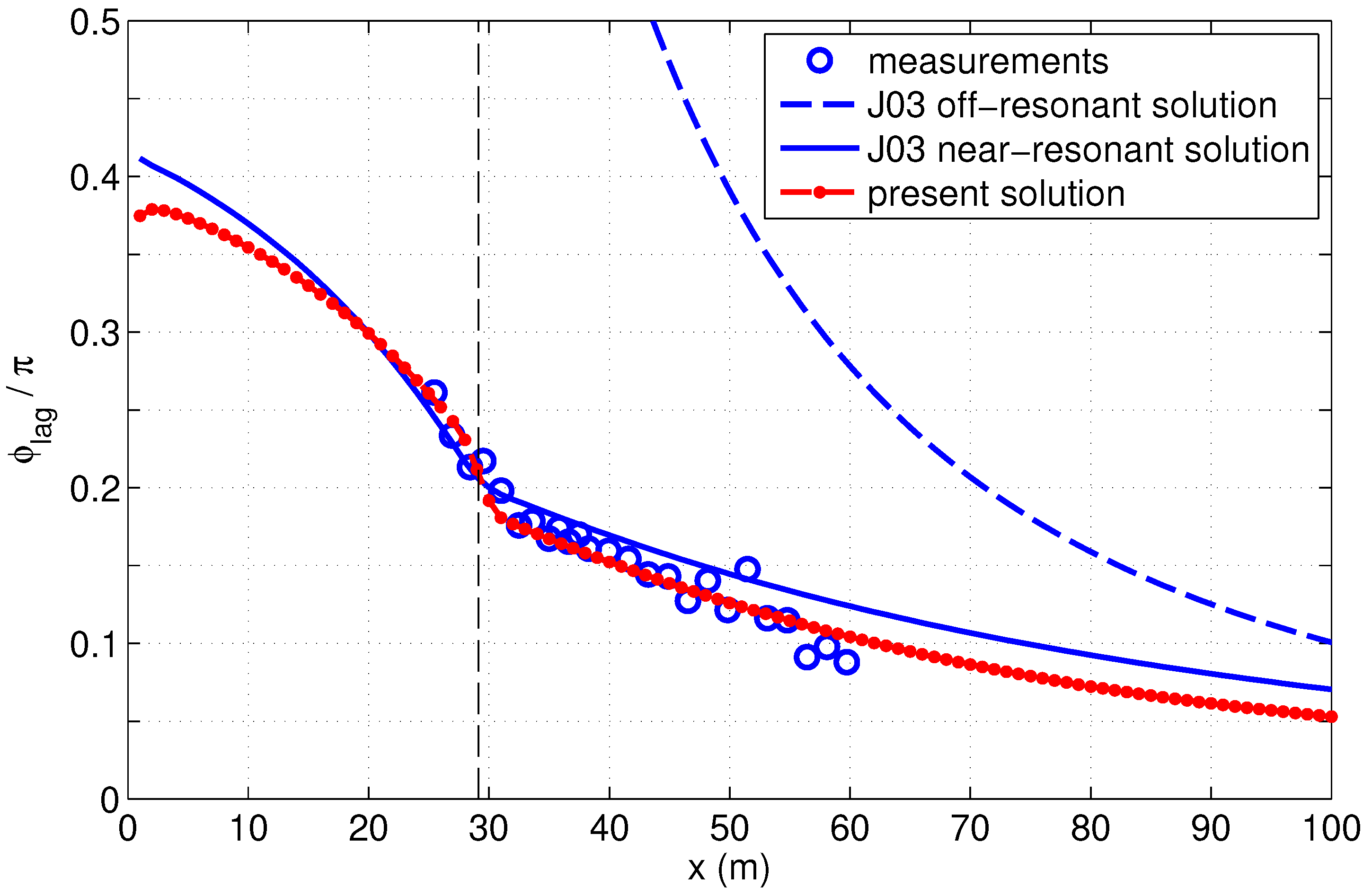
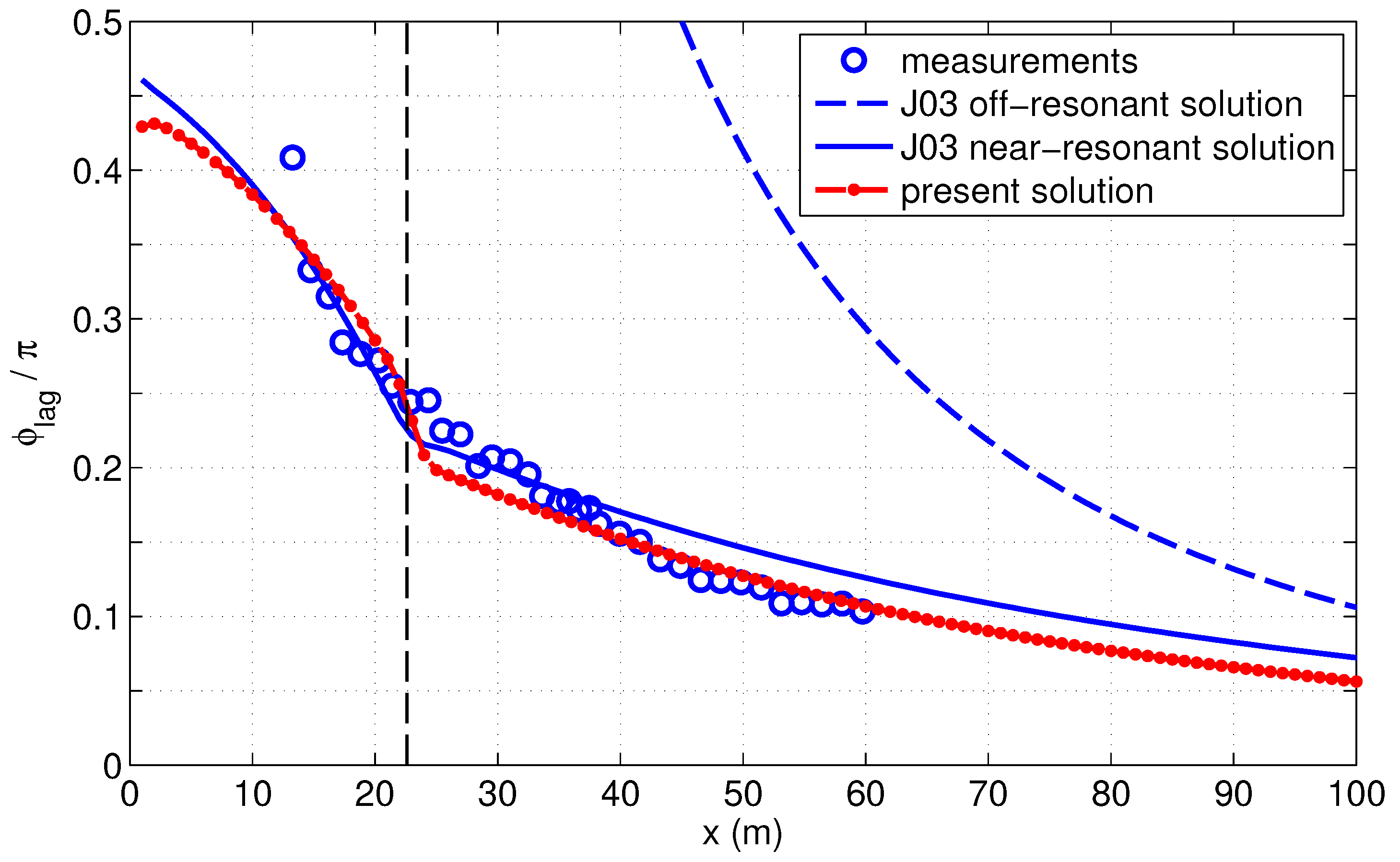
Figure 2,
Figure 3 and
Figure 4 show the measured phase lags for the bichromatic wave conditions B1–B3 compared with both the theoretical solution proposed in the present study (i.e., Equations (
16) and (
17)) and the off-resonant and near-resonant solutions of J03. The breakpoint position indicated on these three figures corresponds to the offshore limit of the breaking zone, which appeared to be a convenient choice for the fixed breakpoint location needed in our theoretical approach. We mention here that the J03 solutions were first replicated according to the bichromatic case considered in their study to ensure our correct computation of these solutions (see
Appendix B).
Figure 5,
Figure 6 and
Figure 7 then show the comparison between measured and theoretical phase lags for the random wave conditions A1–A3, where the mean breakpoint position is indicated. Note that the discrepancy between theory and measurements appeared to increase as the frequency bin considered for the comparison is taken increasingly away from the spectral peak (not shown). A succinct description of these results follows, before enlarging the discussion in
Section 4.
First, the off-resonant solution of J03 can be seen to largely overestimate the phase lag in all conditions. This confirms that, despite its relative straightforwardness to compute because of its local nature (i.e., no integration is required), this solution is not valid in shallow water, as already mentioned by J03. On the contrary, both the theoretical solution proposed in the present study and the near-resonant one of J03 appear to be in close agreement with the measurements, except for bichromatic case B1 where a plateau is observed for the distribution of data points. This unexpected behavior may be related to spurious transverse or cross-mode waves generated close to the breakpoint through resonance in the flume, which induced secondary circulations and therefore modified the mean horizontal velocity field [
29,
30]. The performance skills of the two relevant solutions are synthesized in
Table 2, which globally shows that the present solution yields more accurate phase lag predictions with an overall NRMSE decreasing from 18.1% to 14%, mostly due to a decrease in the overall mean bias (absolute value) from 0.045 to 0.028 rad.
From the measurements, the phase lag is seen to be influenced by the short-wave peak period (compare A1 to A2), by the group period (compare B1 to B2), and by the amplitude modulation (or wave groupiness; compare B2 to B3). The phase lag increases with larger group period and larger short-wave peak period, but decreases with larger wave groupiness. The J03 and the presently proposed solutions do take into account the influence of both the short-wave peak period and the group period on the phase lag, but unfortunately they do not reproduce the observed effect of wave groupiness (more precisely both theoretical solutions appear to be independent of the amplitude modulation). Eventually, the increase of the phase lag when the waves propagate towards shallower water and especially when they enter the surf zone appears to be well reproduced by both theoretical solutions.
While the high-resolution GLOBEX data allowed us to validate both our proposed theoretical solution and the near-resonant one of J03, the latter observations concerning the bound wave phase lag remain tied to the specificity of these experiments. A broader analysis of the phase lag characteristics is thus presented in
Section 4, through an inter-comparison of the two relevant theoretical solutions.
5. Conclusions
The present work provides a new investigation of the bound wave phase lag based on the pioneer and reference work of Schäffer [
12] for modeling group-forced long waves reaching the shore. The proposed semi-analytical solution for the phase lag was tested against the GLOBEX laboratory dataset [
24] involving both bichromatic and random wave conditions over a gently sloping beach, together with the off-resonant and near-resonant solutions of Janssen et al. [
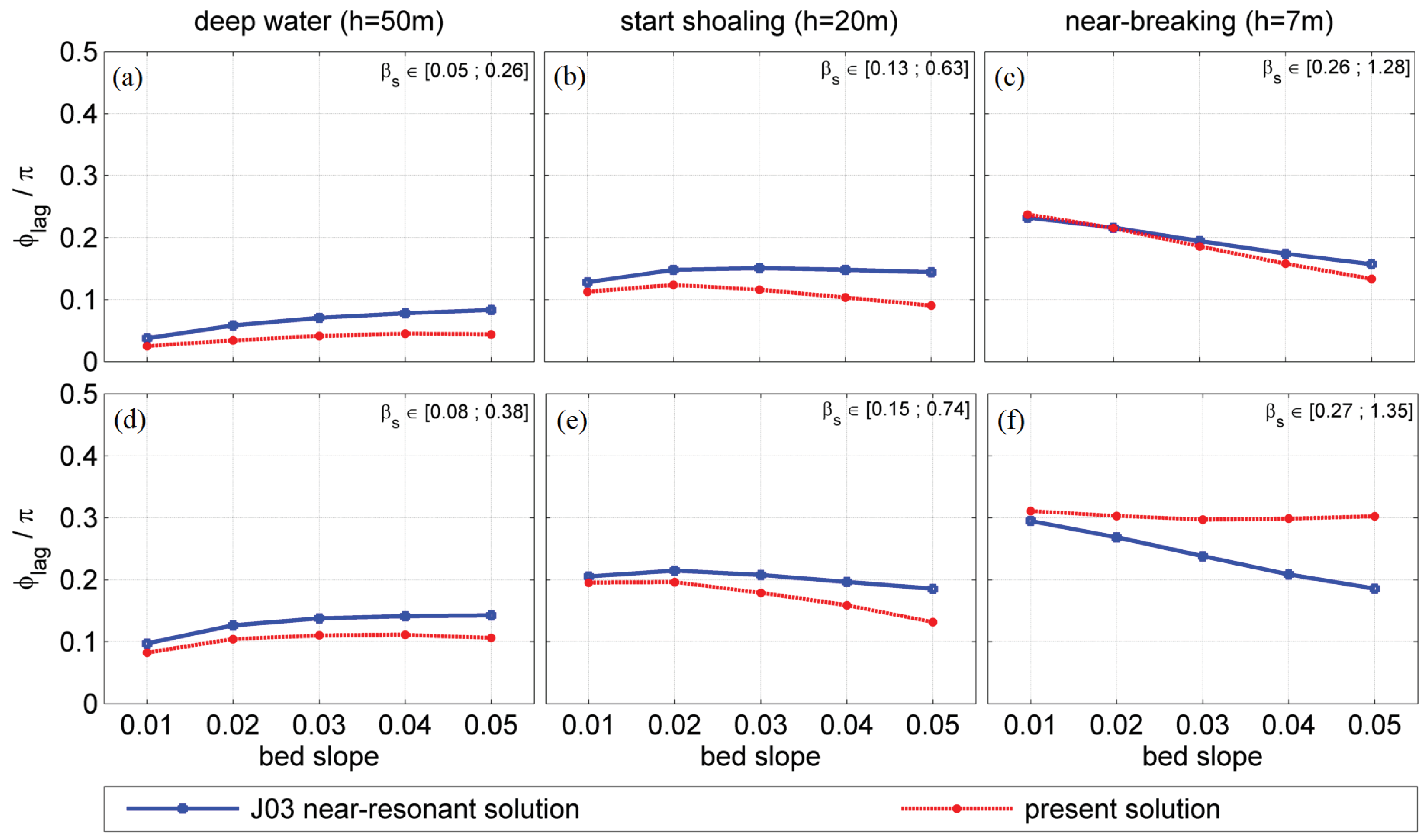
21] (J03). Strong agreement was obtained when comparing the new solution with data for five out of six experiments, while some discrepancy appeared for one experiment (bichromatic conditions B1) due to the presence of an unexpected plateau in the data. In general, despite an occasional slight overestimation of the phase lag in the shoaling zone, these comparisons also extend the applicability of the J03 near-resonant solution to the GLOBEX dataset.
An extensive inter-comparison of our proposed phase lag solution and the one of J03 was performed to investigate in more detail their dependence on the four influencing parameters: the bed slope, the water depth, the incident short-wave peak period and the incident group period. While the bound wave phase lag is mainly seen to increase as the short-wave peak period increases and/or as the water depth decreases, the influence of both the bed slope and the group period on the phase lag is not unequivocal. Indeed, steeper bed slopes induce lower phase lags in shallow water but higher ones in deep water, while higher group periods induce higher phase lags for gentle slopes but lower ones for steep slopes. At the same time, the discrepancy between the two theoretical solutions is seen to increase as the relative bottom slope
increases, in consequence to the first-order approximation in terms of
on which the J03 solution is based. Confronting these phase lag solutions with field data would be of great interest for future studies, provided that the field conditions do not deviate too much from the theoretical framework. In addition, it seems worthwhile also considering the phase difference between the breakpoint-forced long waves and their forcing when analyzing infragravity wave signals in coastal areas [
36].
Finally, as already pointed out in several studies (e.g., [
17,
21,
27]), the growth of IG waves in the nearshore is linked to the phase lag. The interrelated effect of the phase lag on the energy transfer from the short waves to the long waves, which causes the IG waves to grow in amplitude, is thus fundamental to thoroughly understand. While the new insights regarding the bound wave phase lag behavior presented in this work did not allow sufficiently apprehending this relation between phase lag and energy transfers, this important aspect of the IG waves dynamics will hopefully be the focus of a future study.


