Experimental and Numerical Study of Blood Flow in μ-vessels: Influence of the Fahraeus–Lindqvist Effect

Abstract

The study of hemodynamics is particularly important in medicine and biomedical engineering as it is crucial for the design of new implantable devices and for understanding the mechanism of various diseases related to blood flow. In this study, we experimentally identify the cell free layer (CFL) width, which is the result of the Fahraeus–Lindqvist effect, as well as the axial velocity distribution of blood flow in microvessels. The CFL extent was determined using microscopic photography, while the blood velocity was measured by micro-particle image velocimetry (μ-PIV). Based on the experimental results, we formulated a correlation for the prediction of the CFL width in small caliber (D < 300 μm) vessels as a function of a modified Reynolds number (Re_∞) and the hematocrit (H_ct). This correlation along with the lateral distribution of blood viscosity were used as input to a “two-regions” computational model. The reliability of the code was checked by comparing the experimentally obtained axial velocity profiles with those calculated by the computational fluid dynamics (CFD) simulations. We propose a methodology for calculating the friction loses during blood flow in μ-vessels, where the Fahraeus–Lindqvist effect plays a prominent role, and show that the pressure drop may be overestimated by 80% to 150% if the CFL is neglected.

1. Introduction

The characteristics of blood flow in small arteries are of great interest in biomedical engineering. The results of such studies provide information that is useful in understanding in vivo blood flow conditions, in designing medical devices (e.g., organs on a chip), or in the development of more effective diagnostic tools. Although blood flow in large arteries has been extensively studied [1], little work has been done regarding the blood flow in smaller vessels, mainly because both in vivo and in vitro experiments in arterioles and capillaries are difficult to perform. In an experimental study in our laboratory, Anastasiou et al. [2] used a blood substitute, i.e., a fluid that has the viscoelastic properties of blood, and conducted experiments in a D = 600 μm conduit. However, it is well known that in blood vessels with D < 300 μm, the Fahraeus–Lindqvist effect [3,4] must be also taken into account, i.e., during blood flow in such microvessels, the erythrocytes migrate towards the centre of the channel, resulting in the formation of CFL along the vessel wall. The CFL width is defined as the distance from the outer edge of the red blood cell (RBC) core to the luminal surface of the endothelium [5]. This effect has been confirmed by both in-vivo and in-vitro experiments inside glass capillaries [6,7]. Several parameters affect the CFL, such as the diameter of the vessel, H_ct, and flow conditions. The latter can be described by Re_∞, which uses the asymptotic viscosity value, μ_∞. As expected, the CFL exhibits a lower viscosity than the rest of the fluid and this facilitates blood flow through the microvessels. This is clearly pronounced by relevant studies that attempt to estimate wall shear stress [8,9] or pressure drop [10] values in such vessels. Although this phenomenon is significant for diameters less than 300 μm, most of the published work is focused on vessel diameters between 20 and 100 μm, e.g., [6], or on fairly different geometries [11].

Motivated by the importance of these parameters in biomedical engineering, the aim of this study is to provide engineers and physicians with a methodology that could be applied for the prediction of the overall pressure drop (ΔP) and flow characteristics across blood microvessels. To accomplish this, we followed three steps:

• First, estimate the CFL extent. In the relevant published research, either the H_ct value [12] or the vessel diameter [13] was considered when formulating correlations for the prediction of the CFL width. In this study, we investigated the effect of both Re_∞ and H_ct on CFL characteristics in three microvessels with a 50, 100, and 170 μm hydraulic diameter. The experimental data were used for formulating a correlation for estimating the CFL width under the combined effect of the various flow conditions (i.e., Re_∞) and hematocrit values.
• The second one is to investigate the blood velocity profile in such microvessels using the well-established micro-particle image velocimetry (μ-PIV) technique. We employed two different tracing methods, i.e., coloured RBCs or standard PIV tracers. Previous studies suggested that the two tracing methods give significant different results [14]. This issue is clarified in this study. The acquired experimental data was used for validating the computational fluid dynamics (CFD) code.
• The final one is to develop a simplified “two-regions” model using computational fluid dynamics (CFD) by utilizing the outcome of the experimental part of this study in order to set up reliable simulations, a common practice in the literature [15]. The scope of this final step was to calculate the blood flow characteristics as well as the overall pressure drop (ΔP) across the vessels. The CFL flow domain was solved by assuming the blood properties are that of a Newtonian fluid, whereas in the vessel core, the blood rheology is formulated using a non-Newtonian model. Simulations were executed for various blood velocities and vessel diameters.

2. Experimental Procedure

The fluids used in our experiments were mixtures of red blood cells (RBCs) and physiological saline, whose physical properties were similar to those of blood. A small amount of ethylenediaminetetraacetic acid (EDTA), an anticoagulant of choice for hematological applications, was added to prevent coagulation. Consequently, we can assume that the extent of cell aggregation is similar to that of a healthy man. The RBCs were collected from healthy adult volunteers. The experimental study was performed in accordance with the Ethical Guidelines of the Aristotle University of Thessaloniki (European Communities Directive of 24 November 1986-86/609/EEC) for the use of human material in experimental procedures and approved by the Ethical Committee of the School of Dentistry, Aristotle University of Thessaloniki, Thessaloniki, Greece (no. 343/2013). The RBC purification process comprised the following steps:

• Separation of RBCs from plasma by centrifugation (at 3200 rpm) of the whole blood sample.
• Purification of the separated RBCs by washing with saline water and centrifuging twice.

The acquired RBCs were then used to produce “blood” of a known H_ct. The composition of all fluids used in our experiments are presented in

Table 1. Fluids’ composition (% v/v).

Fluid	Red Blood Cell (RBC)	Saline	EDTA
H10	10	89.5	0.5
H20	20	79.5	0.5
H30	30	69.5	0.5
H40	40	59.5	0.5

. The viscosity of the samples was measured using a cone plate rheometer (AR-G2, TA Instruments) at 24 °C. To verify the similarity with “real” blood, the measured viscosity of the samples was compared to the Quemada model (Equation (1)) [16]:

$$\mu =\frac{{\mu }_p}{{(1-0.5\cdot k\cdot H_{ct})}^2},$$

(1)

$$\mathrm{where}k=\frac{k_0+k_{\infty }\cdot \sqrt{{\gamma }_r}}{1+{\gamma }_r},$$

(2)

$$\mathrm{and}{\gamma }_r=\frac{\gamma }{{\gamma }_c},$$

(3)

where k₀, k_∞, and γ_c are, in general, functions of hematocrit [17].

From Figure 1, where the Quemada model is compared with the experimental data, it can be deduced that the prepared fluids exhibit non-Newtonian behaviour and can be used as blood analogues.

It is known that RBCs absorb light. The areas of low RBC concentration are identified as brighter areas when a light source is placed at the bottom of the micro channel and the flow is recorded from above using a high-speed camera. All experiments were conducted in three channels with a square cross sections measuring 50 × 50, 100 × 100 and 170 × 170 μm, respectively, etched on a Poly(methyl methacrylate) (PMMA) plate and sealed with the same material. Square cross section channels were preferred over cylindrical ones to minimize problems caused by light refraction.

3. Cell Free Layer (CFL) and Velocity Measurements

A widely applied technique for determining the velocity in microvessels is the μ-PIV [2], which is based on measurement of the velocity of tracing particles. The method can determine two-dimensional velocity fields with high accuracy and spatial resolution. The measuring section is illuminated by a double cavity Nd:YAG laser emitting at 532 nm, while the flow is recorded using a high sense CCD camera, connected to a Nikon microscope. Also, a 20X air immersion objective lens with NA = 0.45 is used resulting to 2.8 μm depth of field. The experimental set-up used in this study is presented in Figure 2. Τwo kinds of tracing particles were used in this study, namely:

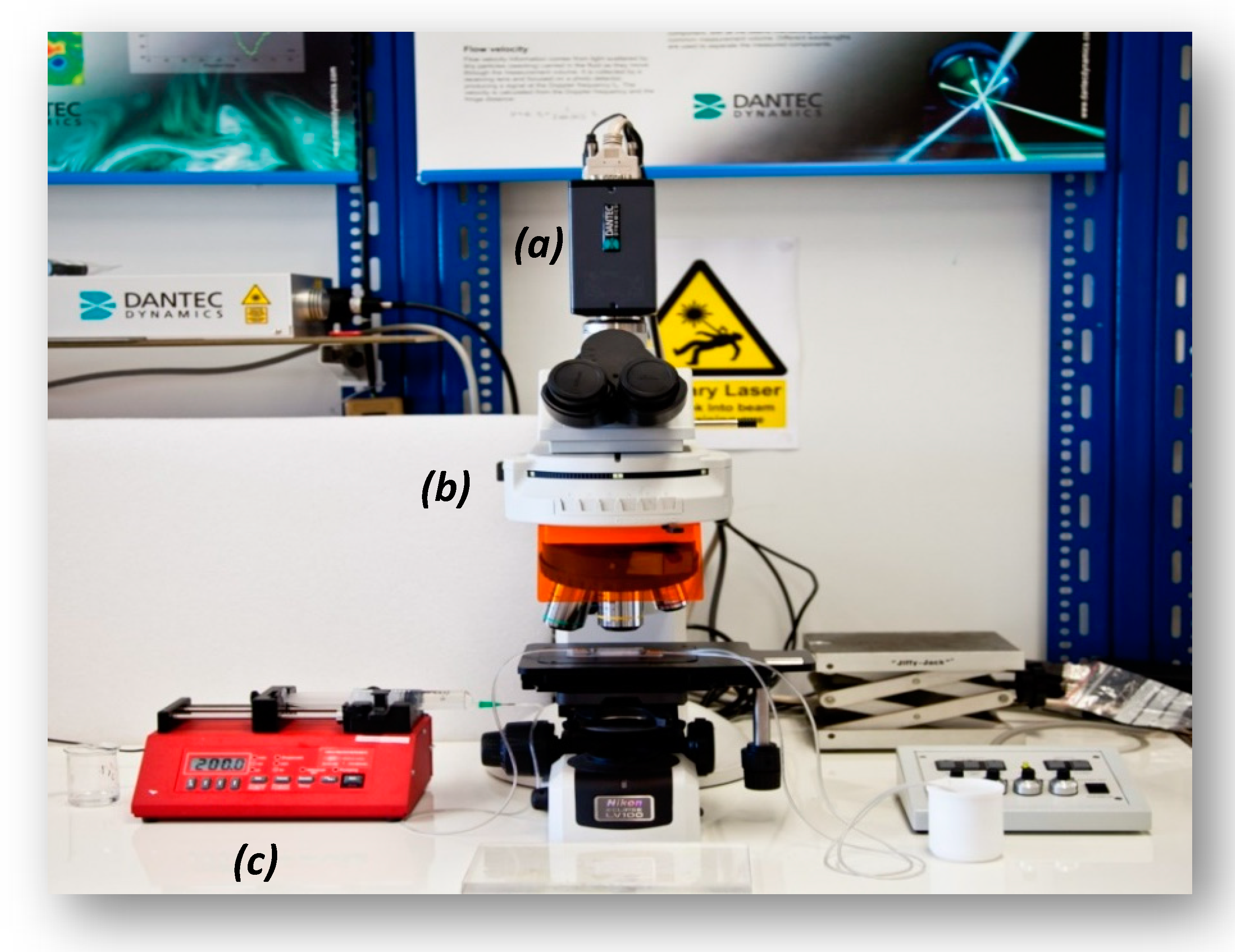
• Spherical fluorescent particles (Invitrogen) with 1.1 μm mean diameter.
• RBCs coloured with fluorescent dye (Rhodamine B).

The fluorescence dye was added to the RBCs right after the centrifugation and before the final mixing with saline water. The measurement of blood velocity can be strongly affected by the settling of RBCs inside the liquid phase. According to Stokes law [18], the settling velocity, U_t (Equation (4)), is a function of the density difference between the two phases, the particle size, and the viscosity of the fluid:

$$U_t=\frac{g_{}^{}({\rho }_p-{\rho }_l)D^2}{18\mu }.$$

(4)

In our experiments the direction of the settling velocity of the erythrocytes was perpendicular to the direction of the fluid velocity as the test section was placed in horizontal position.

An objective of this study was to investigate the effect of hematocrit and flow rate on CFL width. Thus, we performed experiments using RBC dispersions with H_ct 10%, 20%, 30%, and 40% and Re_∞ 0.3–6.0. The reference viscosity used for calculating the Re_∞ is the one obtained from the Quemada model for very high shear rates (γ > 1000 s⁻¹). The effect of the channel diameter on the CFL was investigated by conducting experiments in the three μ-channels. The experimental setup used (Figure 3) employs the microscope of the μ-PIV set up with the same lens, but in this case, the flow was recorded by a high-speed camera.

We determined the CFL at steady-state conditions by acquiring and analysing an appropriate number of consecutive frames and then using the data for the construction of CFL traces and calculation of the average CFL width (Figure 4).

4. Experimental Results

Blood velocity measurements for flow rates ranging from 5 to 10 mL/h, presented in Figure 5, reveal that the axial velocity distribution, i.e., blunted parabolic velocity profiles, is practically the same regardless of the tracing method employed. However, Pitts and Fenech [14],who used the same tracing methods, found a significant difference between the velocities obtained by the two methods. We believe that this discrepancy may be attributed to the low volumetric flow rates they had in their experiments (two orders of magnitude lower than our flow rates). More precisely, for low volumetric flowrates, the settling velocity of the RBCs is of the same order of magnitude as the axial velocity of the main flow. To confirm this belief, we performed experiments with similar flow rates as those reported [14]; that is, 0.01 mL/h, and we recorded the motion of the RBCs at three planes of the micro-channel, i.e., bottom, middle, and top (Figure 6). As the fluid velocity decreases, the settling velocity of the RBCs (vertical velocity component U_t = 6.2 × 10⁻⁴ m/s) is comparable to their horizontal velocity, resulting in the settling of the RBCs before exiting the test section. Thus, instead of a dispersed flow, a separated flow is maintained, where the majority of the RBCs migrate near the bottom, leaving the upper part of the vessel filled with saline. However, in the second method, i.e., the method employing the tracing particles, the settling velocity is much lower (due to the smaller diameter compared to RBCs) and thus they can follow the flow even for very low flow rates.

During μ-PIV measurements, the effect of the out-of-focus particles on the measurements is expressed in terms of the depth of correlation. The depth of correlation is defined as the axial distance from the object plane in which a particle becomes sufficiently out of focus so that its contribution to the signal peak in the particle–image correlation function is neglected [19]. This distance is a function of the characteristics of the objective lens, the diameter of the tracing particles, and the wavelength of the light. For the coloured RBCs and our illumination system, the depth of correlation is estimated to be about 40 μm.

When the RBCs are uniformly distributed throughout the vessel volume, the measured velocity profile is mainly due to the RBCs that lie on the focusing plane and thus the two measuring methods give practically identical results. However, when the RBCs settle, their concentration becomes greater towards the bottom of the microvessel. In this case, the measured velocity is greatly affected by the slow-moving RBCs that lie on a lower plane.

Typical blunted parabolic velocity profiles for various H_ct are shown in Figure 7, where for the same volumetric flow rate, the maximum velocity decreases and the velocity profile becomes blunter as the H_ct is increased. A similar behaviour was also observed in the numerical work of Fedosov et al. [20] and Sriram et al. [21], who both found a great reduction of the maximum axial velocity as H_ct increased.

Figure 8 shows the RMS (root mean square) value of the instantaneous velocity measurement along the middle plane of the conduit reduced with respect to the mean velocity defined as U_mean = Q/A. The detected velocity fluctuations can be attributed to the fact that due to the depth of the field (i.e., approximately 3 μm), particles located on different planes may contribute to the measurement. As expected, the fluctuations are more pronounced in the vicinity of the walls, due to higher axial velocity gradients. The present results clearly show that the RMS value increases with the hematocrit, a fact that is in accordance with the findings of Lima et al. [22] and Lauri et al. [11].

The measurements reveal that that the quantity CFL/D, i.e., the CFL value normalized with respect to the hydraulic diameter, decreases with increasing H_ct, which is in accordance with Namgung et al. [6]. This can be attributed to the fact that as the concentration of the RBCs increases, the viscous forces increase and hinder the movement of the cells in the middle of the channel. Additionally, the normalized CFL decreases as the diameter of the microchannel increases, a fact that is also confirmed by Namgung et al. [6] The results also showed that in the flow rate range where migration started, there is still a low cell concentration near the wall and not a total absence of cells.

We measured the CFL at steady-state conditions by acquiring and analysing an appropriate number of consecutive frames and then we used the data both for the construction of CFL traces (a typical one is presented in Figure 9) and for calculation of the average CFL width and its corresponding standard deviation (SD). Figure 10 shows that the CFL variation increases for low flow velocities, i.e., low pseudo shear rate, and this was confirmed by Kim et al. [16].

Measurements for several volumetric flow rates revealed that the CFL increases by increasing the flow rate until it reaches a constant value for Re_∞ > 4. This can be explained as follows. As the RBCs are migrating towards the centre of the vessel, their concentration increases up to the point where viscous forces hinder additional migration. Using response surface methodology (RSM), a second order polynomial equation, also known as the quadratic model (Equation (5)) [23], is formulated:

$$y=a_0+{\displaystyle \sum _{j=1}^k{a}_j{x}_j}+{\displaystyle \sum _{j=1}^k{a}_{jj}{x}_j^2}+{\displaystyle \sum {\displaystyle \sum _{i\ne j}^k{a}_{ij}{x}_i{x}_j}},$$

(5)

where a₀, a_j, a_jj and a_ij are the unknown coefficient of the polynomial equation, whereas x_i,x_j are the selected design variables. In our case, we calculated the quantity CFL/D as a function of Re_∞ and H_ct (Equation (6)). The values of the coefficients of the polynomial were determined using the experimental data for two (k = 2) variables and are given in

Table 2. Coefficients of the CFL correlation.

Coefficient	Value	Coefficient	Value
a0	0.066384	a11	0.000002
a1	−0.000887	a22	−0.001414
a2	0.017796	a12	−0.000005

:

$$\raisebox{1ex}{$CFL$}\!\left/ \!\raisebox{-1ex}{$D$}\right.=a_0+a_1{H}_{ct}+a_{2}R{e}_{\infty }+a_{11}{H}_{ct}^2+a_{22}R{e}_{\infty }^2+a_{12}{H}_{ct}R{e}_{\infty }.$$

(6)

Equation (6) can predict the quantity CFL/D with uncertainty better than 10% for Re_∞ 0.3 to 6 and H_ct 10% to 40% (Figure 11 and Figure 12). The accuracy of the equation was calculated by comparing the correlation with the experimental results. For Re_∞ > 4, the CFL/D quantity approaches a constant value, which depends on H_ct. The novelty in our approach was the inclusion of two parameters, namely Re_∞ and H_ct, in the proposed correlation, a combination that is often omitted in existing research [12,13] but adds a significant amount of credibility in the proposed model.

CFL/D values predicted by the proposed correlation were found to be in good agreement with the limited published experimental data [24] (Figure 13).

5. CFD Simulations

In our simulations, the Fahraeus effect [25] was taken into consideration and was modelled using a relative correlation (Equation (7)) [26]:

$$\begin{array}{c}\frac{H_T}{H_{ct}}=H_{ct}+\left(1-H_{ct}\right)\left(1+1.7e^{-0.415D}-0.6e^{-0.011D}\right),\end{array}$$

(7)

where $H_T$, is the tube hematocrit in the microvessel caused by the Fahraeus effect.

The RBC concentration, i.e., the local $H_{ct}$ value, was modelled using the Lih [27] model distribution, fitted for each case, as shown in Equation (8):

$$\begin{array}{c}{H}_{ct}\left(r\right)=H_m{\left(1-\frac{r}{D/2}\right)}^6,\end{array}$$

(8)

where r is the radius and $H_m$ is the mean hematocrit value in the core area for each case.

The blood density was set at a constant value (ρ_b = 1050 kg/m³). In the CFL zone, blood was modelled as a Newtonian fluid having the viscosity of human blood plasma (μ_p = 1.2 cP), whereas, in the core area blood, it was modelled as non-Newtonian shear thinning fluid. This was achieved through a modified Quemada model, where local μ is expressed by Equation (1), K is expressed by Equation (2), and its coefficients ($k_0,k_{\infty },{\gamma }_c$) are expressions of $H_{ct}$ as formulated by Das et al. [17], described in Equations (9)–(11):

$$\begin{array}{c}{k}_0=m_0+\frac{2}{m_1+\phi },\end{array}$$

(9)

$$\begin{array}{c}{k}_{\infty }=\exp \left(b_0+b_1\phi +b_2{\phi }^2+b_3{\phi }^3\right),\end{array}$$

(10)

$$\begin{array}{c}\dot{{\gamma }_c}=\exp \left(c_0+c_1\phi +c_2{\phi }^2+c_3{\phi }^3\right),\end{array}$$

(11)

where φ = $H_{ct}\left(r\right)/100.$ The remaining constants are presented in

Table 3. Coefficients used in Equations (9)–(11).

Coefficient	Value	Coefficient	Value
$m_0$	0.275363	$m_1$	0.100158
$b_0$	1.3435	$b_1$	−2.803
$b_2$	2.711	$b_3$	−0.6479
$c_0$	−6.1508	$c_1$	27.923
$c_2$	−25.60	$c_3$	3.697

.

A typical viscosity distribution, representative of the above model, is shown in Figure 14a. CFD modelling in this study was conducted using the ANSYS CFX commercial code (v. 19, ANSYS Inc., Canonsburg, PA, USA).

The blood vessels (length (L) = 2 mm) were modelled as two-dimensional computational domains with axial symmetry and an adjustable radius (R). The geometry of the domain and the mesh were designed on the ANSYS Workbench package. The blood flow was designed as a single computational domain, where all the blood properties and the flow characteristics varied continuously. Namely, the viscosity alteration between the Newtonian CFL and the non-Newtonian core was modelled using a steep sigmoid curve, in order to avoid numerical instabilities on the CFL border (Figure 14a). As Re_∞ values are low, the flow is laminar. Thus, the direct numerical simulation (DNS) model was used, while the high-resolution advection scheme was employed for the discretization of the momentum equations. The simulations were run in steady state, the vessel walls were considered smooth, and a no-slip boundary condition was imposed. At the inlet, constant velocity, i.e., a Dirichlet boundary condition, was imposed. The outlet pressure was set constant and equal to atmospheric. As for the meshing procedure, an optimum grid density was chosen by performing a grid-dependency study. The inlet pressure was used as a parameter for the grid-dependency study. Typical results are presented in

Table 4. Grid dependency study results (D = 50 μm, Re_∞ = 4.9).

Maximum Cell Face Size (μm)	Inlet Pressure (Pa)
5.0	2610
4.0	2578
3.0	2555
2.5	2553

. Furthermore, the mesh was refined along the CFL border, where viscosity changes are more pronounced. Consequently, cells with a maximum face size of 2.5 μm were used, while mesh refinement was applied in areas where viscosity changes were pronounced, e.g., near the wall.

Simulations were performed for diameters varying between 50 and 170 μm, H_ct between 10% and 40%, and Re_∞ between 0.3 and 5. In Figure 14b, the blood viscosity distribution is illustrated for one of the cases tested (D = 100 μm, Re_∞ = 0.8, H_ct = 30%). In the CFL zone, depicted in blue colour, the viscosity is that of blood plasma, whereas in the non-Newtonian core, the viscosity gradually decreases as the radial distance increases.

The CFD results were compared with our relevant experimental data (Figure 15). It is evident that the CFD results are in very good agreement with the corresponding experimental data. In Figure 16, the data by Gaehtgens et al. [28] concerning axial velocity distribution are compared with the corresponding CFD case (i.e., D = 80 μm, Re_∞ = 0.3, H_ct = 37%). There seems to be a relatively good agreement between the experimental and computational results, bound with deviations less than 5%.

Additionally, during the CFD simulations, the overall pressure drop (ΔP_CFL) in various vessels was calculated across the whole length of the vessel and was compared with three values, namely:

• The ΔP_HP, calculated analytically using the Hagen–Poiseuille equation for straight circular tubes and considering the blood as a Newtonian fluid (e.g., μ_∞ = 3.5 cP for H_ct = 40%).
• The ΔP_nCFL calculated numerically considering that there is no CFL and that the blood behaves as a non-Newtonian fluid (in the same way the non-Newtonian core was modelled) [29].
• The ΔP_[10] calculated iteratively using the equations proposed in [10], considering blood as a Casson fluid.

As presented in

Table 5. Pressure drop for various cases.

Re∞	D (μm)	Hct (%)	ΔPCFL (Pa)	ΔPnCFL (Pa)	ΔPHP (Pa)	ΔP[10] (Pa)	ΔPnCFL/ΔPCFL	ΔPHP/ΔPCFL
0.8	100	30	132	238	302	184	1.8	2.29
1.4	170	40	42	103	105	67	2.5	2.50
2.5	170	40	105	187	186	117	1.8	1.77
4.9	170	40	204	377	372	229	1.8	1.82
1.2	50	20	1463	2753	2984	1629	1.9	2.04
1.1	50	40	1466	2772	3256	1978	1.9	2.22

, omitting consideration of the existence of CFL in vessels where the Fahraeus–Lindqvist effect occurs leads to overestimation of pressure drop values by 80% to 150%.

It is obvious that the main factor influencing the pressure drop in such vessels is the wall frictions, via the wall shear stresses, which in turn, is highly affected by the fluid viscosity and the velocity gradient near the wall. As shown in Figure 7, the near-wall velocity distribution seems to be the same regardless of the hematocrit value. This could possibly explain the fact that wall frictions in vessels where the CFL is present are practically independent of the hematocrit value. Lastly, it is evident that there is good accordance between our estimated pressure drop values with values calculated using the methodology proposed by Chandran et al. [10], where the deviation is between 10% and 30%.

6. Conclusions

It is known that the calculation of the pressure drop in small calibre blood vessels (i.e., D < 300 μm), which is directly related to the wall shear stress, is not straight forward and it is a rather difficult task. Based on the acquired experimental data, a correlation for predicting CFL was formulated and its validity was checked with published experimental data. This correlation along with the lateral distribution of $H_{ct}$ can be used as input to the CFD code. The reliability of the code is further supported by the very good agreement between the experimentally obtained axial velocity profiles and those calculated by the CFD simulations.

In the present study, we proposed a methodology for calculating the friction loses during blood flow in microvessels, where the Fahraeus–Lindqvist effect is prominent. In cases that the blood hematocrit and the flow conditions (Re_∞) are known, someone can utilize the proposed correlation (Equation (6)) to predict the CFL width. In the CFL zone, blood is modelled as a Newtonian fluid having the viscosity of blood plasma, whereas in the core area, blood is modelled as a non-Newtonian shear thinning fluid. Consequently, a complicated problem, the Fahraeus–Lindqvist effect, which occurs during blood flow, is now simplified to a single-phase flow simulation that can converge relatively fast without the need of high computational power. The results of the CFD simulation give valuable information, like the pressure drop, in blood μ-vessels and wall shear stress estimation.

A possible next step of the current study would be to formulate a generalised expression for the prediction of the friction factor for blood flow in microcirculation, including the Fahraeus–Lindqvist phenomenon, in an attempt to modify already existing models [29].

References

1. Tuma, R.F.; Duran, W.N.; Ley, K. Microcirculation; Academic Press: Cambridge, MA, USA, 2011; ISBN 978-0-08-056993-2. [Google Scholar]
2. Anastasiou, A.D.; Spyrogianni, A.S.; Koskinas, K.C.; Giannoglou, G.D.; Paras, S.V. Experimental investigation of the flow of a blood analogue fluid in a replica of a bifurcated small artery. Med. Eng. Phys. 2012, 34, 211–218. [Google Scholar] [CrossRef] [PubMed]
3. Fåhræus, R.; Lindqvist, T. The viscosity of the blood in narrow capillary tubes. Am. J. Physiol.-Leg. Content 1931, 96, 562–568. [Google Scholar] [CrossRef]
4. Albrecht, K.H.; Gaehtgens, P.; Pries, A.; Heuser, M. The Fahraeus effect in narrow capillaries (i.d. 3.3 to 11.0 μm). Microvasc. Res. 1979, 18, 33–47. [Google Scholar] [CrossRef]
5. Ong, P.K.; Namgung, B.; Johnson, P.C.; Kim, S. Effect of erythrocyte aggregation and flow rate on cell-free layer formation in arterioles. Am. J. Physiol. Heart Circ. Physiol. 2010, 298, H1870–H1878. [Google Scholar] [CrossRef] [PubMed]
6. Namgung, B.; Ju, M.; Cabrales, P.; Kim, S. Two-phase model for prediction of cell-free layer width in blood flow. Microvasc. Res. 2013, 85, 68–76. [Google Scholar] [CrossRef]
7. Pries, A.R.; Schönfeld, D.; Gaehtgens, P.; Kiani, M.F.; Cokelet, G.R. Diameter variability and microvascular flow resistance. Am. J. Physiol. Heart Circ. Physiol. 1997, 272, H2716–H2725. [Google Scholar] [CrossRef]
8. Sriram, K.; Intaglietta, M.; Tartakovsky, D.M. Non-Newtonian Flow of Blood in Arterioles: Consequences for Wall Shear Stress Measurements. Microcirculation 2014, 21, 628–639. [Google Scholar] [CrossRef]
9. Balogh, P.; Bagchi, P. Three-dimensional distribution of wall shear stress and its gradient in red cell-resolved computational modeling of blood flow in in vivo-like microvascular networks. Physiol. Rep. 2019, 7, e14067. [Google Scholar] [CrossRef]
10. Chandran, K.B.; Rittgers, S.E.; Yoganathan, A.P.; Rittgers, S.E.; Yoganathan, A.P. Biofluid Mechanics: The Human Circulation, 2nd ed.; CRC Press: Boca Raton, MA, USA, 2012; ISBN 978-0-429-10607-1. [Google Scholar]
11. Lauri, J.; Bykov, A.; Fabritius, T. Quantification of cell-free layer thickness and cell distribution of blood by optical coherence tomography. J. Biomed. Opt. 2016, 21, 040501. [Google Scholar] [CrossRef]
12. Sriram, K.; Vázquez, B.Y.S.; Yalcin, O.; Johnson, P.C.; Intaglietta, M.; Tartakovsky, D.M. The effect of small changes in hematocrit on nitric oxide transport in arterioles. Antioxid. Redox Signal. 2011, 14, 175–185. [Google Scholar] [CrossRef]
13. Al-Khazraji, B.K.; Jackson, D.N.; Goldman, D. A Microvascular Wall Shear Rate Function Derived From In Vivo Hemodynamic and Geometric Parameters in Continuously Branching Arterioles. Microcirculation 2016, 23, 311–319. [Google Scholar] [CrossRef] [PubMed]
14. Pitts, K.L.; Fenech, M. High speed versus pulsed images for micro-particle image velocimetry: A direct comparison of red blood cells versus fluorescing tracers as tracking particles. Physiol. Meas. 2013, 34, 1363–1374. [Google Scholar] [CrossRef] [PubMed]
15. Sharan, M.; Popel, A.S. A two-phase model for flow of blood in narrow tubes with increased effective viscosity near the wall. Biorheology 2001, 38, 415–428. [Google Scholar] [PubMed]
16. Kim, S.; Kong, R.L.; Popel, A.S.; Intaglietta, M.; Johnson, P.C. Temporal and spatial variations of cell-free layer width in arterioles. Am. J. Physiol. Heart Circ. Physiol. 2007, 293, H1526–H1535. [Google Scholar] [CrossRef] [PubMed] [Green Version]
17. Das, B.; Johnson, P.C.; Popel, A.S. Effect of nonaxisymmetric hematocrit distribution on non-Newtonian blood flow in small tubes. Biorheology 1998, 35, 69–87. [Google Scholar] [CrossRef]
18. Batchelor, G.K. An Introduction to Fluid Dynamics; Cambridge University Press: Cambridge, UK, 2000; ISBN 978-0-521-66396-0. [Google Scholar]
19. Wereley, S.T.; Meinhart, C.D. Micron-Resolution Particle Image Velocimetry. In Microscale Diagnostic Techniques; Breuer, K.S., Ed.; Springer: Berlin/Heidelberg, Germany, 2005; pp. 51–112. ISBN 978-3-540-26449-1. [Google Scholar]
20. Fedosov, D.; Caswell, B.; Popel, A.S.; Karniadakis, G. Blood Flow and Cell-Free Layer in Microvessels. Microcirculation 2010, 17, 615–628. [Google Scholar] [CrossRef] [Green Version]
21. Sriram, K.; Tsai, A.G.; Cabrales, P.; Meng, F.; Acharya, S.A.; Tartakovsky, D.M.; Intaglietta, M. PEG-albumin supraplasma expansion is due to increased vessel wall shear stress induced by blood viscosity shear thinning. Am. J. Physiol. Heart Circ. Physiol. 2012, 302, H2489–H2497. [Google Scholar] [CrossRef] [Green Version]
22. Lima, R.; Wada, S.; Takeda, M.; Tsubota, K.; Yamaguchi, T. In vitro confocal micro-PIV measurements of blood flow in a square microchannel: The effect of the haematocrit on instantaneous velocity profiles. J. Biomech. 2007, 40, 2752–2757. [Google Scholar] [CrossRef] [Green Version]
23. Box, G.E.P.; Wilson, K.B. On the Experimental Attainment of Optimum Conditions. J. R. Stat. Soc. Ser. B Methodol. 1951, 13, 1–45. [Google Scholar] [CrossRef]
24. Reinke, W.; Gaehtgens, P.; Johnson, P.C. Blood viscosity in small tubes: Effect of shear rate, aggregation, and sedimentation. Am. J. Physiol. 1987, 253, H540–H547. [Google Scholar] [CrossRef]
25. Fåhraeus, R. The suspension stability of the blood. Physiol. Rev. 1929, 9, 241–274. [Google Scholar] [CrossRef]
26. Pries, A.R.; Secomb, T.W.; Gaehtgens, P.; Gross, J.F. Blood flow in microvascular networks. Experiments and simulation. Circ. Res. 1990, 67, 826–834. [Google Scholar] [CrossRef]
27. Lih, M.M. A mathematical model for the axial migration of suspended particles in tube flow. Bull. Math. Biophys. 1969, 31, 143–157. [Google Scholar] [CrossRef]
28. Gaehtgens, P.; Meiselman, H.J.; Wayland, H. Velocity profiles of human blood at normal and reduced hematocrit in glass tubes up to 130 μ diameter. Microvasc. Res. 1970, 2, 13–23. [Google Scholar] [CrossRef]
29. Mouza, A.A.; Skordia, O.D.; Tzouganatos, I.D.; Paras, S.V. A Simplified Model for Predicting Friction Factors of Laminar Blood Flow in Small-Caliber Vessels. Fluids 2018, 3, 75. [Google Scholar] [CrossRef]
Figure 1. Experimental data of “blood” viscosity vs. shear rate compared with the Quemada correlation (Hct = 40%).
Fluids 04 00143 g001
Figure 2. Micro-particle image velocimetry (μ-PIV) experimental setup used in this study (a): high-speed camera, (b): microscope, (c): syringe pump.
Fluids 04 00143 g002
Figure 3. Depiction of the: (a) cell free layer (CFL) measurement setup used in our study, (b) detail of the test section.
Fluids 04 00143 g003
Figure 4. Typical images for: (a) Q = 0.5 mL/h; (b) Q = 1.2 mL/h. (D = 100 μm, Hct = 20%) and (c) identification of the CFL boundaries and measurement of its width (Δ).
Fluids 04 00143 g004
Figure 5. Typical velocity profiles for Hct = 10% for both tracing methods (microparticles vs. RBCs) employed (D = 170 μm, Q = 5 mL/h). Comparison shows that the RBC slip velocity is practically zero.
Fluids 04 00143 g005
Figure 6. Typical images: (a) at the bottom of the micro-channel, (b) in the middle, and (c) at the top of the channel. (D = 170 μm, Hct = 10%, Q = 0.01 mL/h).
Fluids 04 00143 g006
Figure 7. Typical velocity profiles at D = 170 μm for three different Hct values (Q = 10 mL/h) using the micro particle method.
Fluids 04 00143 g007
Figure 8. RMS/Umean variation for Hct = 10% and 20% with respect to the radial position (Q = 5 mL/h, D = 170 μm).
Fluids 04 00143 g008
Figure 9. Typical CFL traces for Q = 0.3 and 1.0 mL/h; Hct = 20%, D = 100 μm (wall y = 0 μm).
Fluids 04 00143 g009
Figure 10. Typical variation of CFL standard deviation (SD) vs. pseudo shear rate (Hct = 10%, D = 100 μm).
Fluids 04 00143 g010
Figure 11. Comparison of the current correlation (Equation (6)) with CFL experimental data of this study for: (a) Hct = 10% and (b) Hct = 20% (7% error bars).
Fluids 04 00143 g011
Figure 12. CFL thickness dependence on Hct and Re based on the proposed correlation (Equation (6)).
Fluids 04 00143 g012
Figure 13. Comparison of Equation (6) with Reinke et al.’s [24] experimental data for CFL thickness (10% error bars).
Fluids 04 00143 g013
Figure 14. (a) Radial viscosity distribution (Hct = 10%, Re = 4.4); (b) graphical representation of the viscosity distribution on a cross section (Re = 0.8, Hct = 40%).
Fluids 04 00143 g014
Figure 15. Comparison of computational and experimental velocity results for three cases with D = 170 μm: (a) Hct = 20%, Re = 2.1; (b) Hct = 20%, Re = 4.2; (c) Hct = 10%, Re = 2.1.
Fluids 04 00143 g015
Figure 16. Comparison of numerically calculated axial velocity with published experimental data [28] (D = 80 μm, Re = 0.3, Hct = 37%).
Fluids 04 00143 g016