1. Introduction
In the field of fluid mechanics, experimental techniques for the measurement of velocity play a crucial role. Non-intrusive techniques such as particle image velocimetry (PIV) continue to develop year-on-year. With the advent of high-speed optical diagnostics equipment and ever more powerful processing equipment, the potential data yield has never been higher. However, a persistent problem in any experimental technique is how to deal with erroneous data. In PIV experimental data this often is realised as single spurious vectors or sparse velocity regions.
The causes of spurious vectors are myriad and varied; sub-optimal experimental set-up, misaligm ent of optics, mismatched sheet thickness, high external noise (such as background light and reflections/glare), seeding density inhomogeneity, choice of processing parameters such as window size for example. Some presence of erroneous vectors is inevitable regardless of how competently the experiments are carried out. Therefore, research and development effort in this area focuses on the identification and replacement of spurious vectors during vector post-processing [
1].
One of the first and still most commonly used techniques is based on a local test where vectors are compared to their neighbouring vectors to identify potential outliers based on significant deviations in magnitude or direction. Many variations of ‘tests’ are suggested in literature [
2,
3,
4], including the widely used local median test [
5]. Once spurious vectors have been detected and removed, interpolation methods are then typically used to replace the removed vector and smoothing applied [
1].
Due to the significance placed on experimentally obtained velocity measurements, research on alternative methods for both improved detection and replacement of spurious vectors is on-going. As a starting point, multiple studies suggest how human sight is able to very effectively identify outliers [
6]. Thus, some approaches are based around this idea. Velocity gradients and thresholds form the basis for some techniques [
3,
7], others consider adaptive local coherency [
8].
Similarly, artificial neural networks (ANNs), consisting of elements or neurons are commonplace in many image analysis and computer vision processes. Liang et al. presents a technique using cellular neural networks, claiming the technique offers improved identification of spurious vectors when compared to median methods due to simulating the procedure through which the human brain detects vector errors [
9].
Once spurious vectors are detected, there must be a procedure for determining the replacement vector. For some processes, the same proposed techniques may both detect spurious vectors and offer a replacement. Statistical based approaches such as the penalized least-squares method [
10] or Kriging regression [
11] are two such techniques. More recently, proper orthogonal decomposition (POD) based techniques have been introduced for the purpose of invalid vector detection and replacement, named POD-OC (outlier correction). Wang et.al. [
12] uses low-order POD modes to construct a reference velocity field allowing for outlier detection and correction using an iterative approach, assuming instantaneous spurious vectors will not influence the lower order modes. The approach requires iteration of the POD calculation and includes a user-defined parameter.
Higham et al. [
13] remark on the computational expense of iterative POD-OC methods and propose a non-iterative method (PODDEM). This is achieved through the analysis of generated temporal coefficients, specifically a spike detection. However, the authors suggest that their current approach is most suited to datasets with outliers in every vector field; suggesting that if this is not the case, alternative approaches to spike detection should be carried out. Further, the authors remark on the requirement of a user-defined parameter which impacts the accuracy of the estimation, t
r which they suggest may be estimated from a visual inspection of the PIV data.
The currently presented work introduces the two-point statistical technique, linear stochastic estimation (LSE) as an alternative vector post-processing routine to identify and replace spurious vectors in grid velocity vector fields such as those obtained through PIV measurements without the need for multiple iterations or user defined parameters. Replacement of vectors in such a manner allows their inclusion in the calculation of any derived parameters required such as turbulent kinetic energy (TKE). LSE is discussed in the context of fluid mechanics research and mathematically defined. The vector replacement methodology (LSEVR) is then introduced and described in the application to PIV data. Finally, the performance of the technique is compared to the widely used interpolation approach.
2. Linear Stochastic Estimation
Linear stochastic estimation was introduced to the field of turbulent fluid flows by Adrian [
14,
15] as a way to approximate conditional averages of turbulent flow. In brief, the LSE technique exploits the conditional (or instantaneous) information contained within a flow and its relationship with the two-point correlation tensor,
to allow estimations within the flow. It should be noted that there is a class of techniques related to LSE that use higher-order correlations; quadratic stochastic estimation (QSE). However as well as the increase in computational demand there is often little improvement to be gained from these approaches [
16]. Therefore, application in the presented work will be using the linear, or first order technique (LSE).
In fluid mechanics the LSE technique has found many beneficial applications. A typical application is the replacement of high spatial density measurements—such as PIV—with simpler sensors such as microphones [
17] or wall mounted pressure arrays [
18,
19,
20,
21]. In each of these studies, the correlation between planar velocity measurements and the sensor readings is determined. This in turn allows synchronised estimation of velocity from only the sensor measurements. The limitation of using this sensor type is described, particularly the importance of the proximity and distribution of these sensors [
22].
Further, given flow field knowledge a priori, sensor location may be optimised to improve correlation [
23] provided there is flexibility regarding selection of sensors. As an alternative, point velocity measurements may be used to predict velocity elsewhere in the velocity vector field [
24]. By using velocity as a sensor in this manner there is an increase in correlation between the field and sensors within it. However it is shown that despite the increased spatial correlation of velocity, the proximity of sensors and the location of vectors to be estimated is significant [
25]. Therefore, for the application presented here, the sensor locations should be carefully considered. However, unlike other interpolation-based techniques the adjacent vectors (provided they are not used as sensors) have no impact on the estimation, allowing the technique to be used in regions with more than a single, isolated spurious vector.
In application, LSE is often combined with Proper orthogonal decomposition. The two techniques are complementary given that POD may identify coherent motions, represented as lower order, higher energy modes, while LSE can effectively estimate these structures from a reduced dataset. Butcher and Spencer reveal a coupling due to this effect [
24]. Druault and Guibert introduce the combination of POD and LSE for the purpose of the replacement of spurious vectors [
26]. It is important to note that when POD filtering data, small scale structures are effectively removed, leaving only coherent, typically large-scale motions. Druault and Guibert show how these structures are successfully estimated using the combination of POD and LSE. However, as several of the approaches in literature such as POD-OC and PODDEM require user defined inputs [
13], in order to develop a robust vector replacement approach, they will not be considered further within the presented work.
The application of LSE is best described in two steps. Firstly, the correlation matrix, ‘
a’ is computed. This describes the relationship between each sensor and the location where an estimation is desired. For this step, a valid data set is required with good data at all sensor locations and the location of desired estimation simultaneously—in the case of PIV experimental data, the time series may be scanned to compile a set of valid snapshots (referred to as slave fields). The calculation of the correlation matrix is defined by Equation (1) where
u,
p and
NS are velocity, sensor reading and number of sensors respectively.
Equation (2) defines how the correlation matrix is combined with values at the sensor locations to generate the estimation, where
uest is the estimated velocity.
According to the definition, it is possible to use one velocity component in the estimation of another, i.e., using a cross-correlation—this term is often weaker than a correlation with the same velocity component—therefore the estimations should when possible be calculated for each required velocity component independently.
3. Vector Replacement Methodology
In the current section, the LSE vector replacement methodology (LSEVR) is described and demonstrated on a PIV test case. The performance of LSEVR is then compared to commonly used techniques.
The LSEVR methodology deals only with the replacement of an identified invalid vector and not the identification process itself and therefore this section will cover the replacement of vector which is already identified as spurious (or sparse). By implication, LSEVR may only be used as part of an iterative PIV process after the first pass which would identify spurious vectors.
To apply the LSE technique, it is important that there exist valid data at some time at the point of interest. Therefore, any perpetually occurring invalid regions may not be corrected using the suggested technique. Whilst this requirement seems obvious, its implications are not trivial in the intended application of the correction of spurious experimental data. Common experimental set-up issues such as glare, shadows or insufficiently illuminated regions may not be corrected with this technique, in these cases it is possible that other methods such as interpolation may perform sufficiently. However, it is expected that regions in which there are incidentally sparse multiple vector measurements, LSEVR would perform favourably. Therefore, the first step of the technique is to assess the suitability of the site.
Assuming the vector meets the criteria, information about the vector’s relationship with the surrounding vector field should be determined. Two-point statistics and in-particular the cross-correlation function (CCF) coefficient provides a suitable metric for this purpose. At each point in the flow, the CCF coefficient,
Rij may be calculated according to Equation (3) where subscripts
i and
j are velocity components to be correlated,
r and
τ are the separation in space and time respectively. In this context, only the spatial correlation is required and therefore
τ = 0.
The integral length scales may then be calculated in each direction,
k and for each velocity component,
i and
j. Integrating
Rij according to Equation (4) provides the length scales but in practice is only evaluated up until the first zero crossing of
Rij. In the case of 2D/2C experimental data there are four length scales. For 3D/3C experiments there are nine.
As there are four resulting length scales, they may be used as a guide or limit for the distribution of LSEVR sensors. I.e., sensors should not be selected that sit outside of the area defined by these length scales. It is possible to bypass this calculated and computational expense, if there is an understanding of the flow dynamics a priori which allow a suitable region size to otherwise be defined.
Within the region defined, a number of valid vectors surrounding the one to be replaced should be identified; there is no requirement for these to be immediately adjacent and it may be beneficial for them not to be due to proximity effects [
25].
At all other instances, and where only valid data at the site of uest and sensors exist, Equation (1) should be applied to calculate the correlation matrix, ar which relates each sensor location to the uest site. The ar matrix may be combined with sensor values according to Equation (2) to generate a replacement vector, uest.
The LSEVR process may be summarised in the following steps:
Check probability density of spurious/sparse occurrences at the site
For valid only instances generate spatial correlation distribution and assess length scales in region
Select number of sensors within region of high-correlation (i.e., within length scale) analogous to a filter region size in other approaches. These locations should be valid at instance of required replacement
For valid only instances generate ar matrix using Equation (1)
At the instance of required replacement, use sensors combined with ar matrix according to Equation (2) to generate estimated velocity component(s)
It should be noted that while points 1–5 above describe the full approach for LSEVR, it is possible to carry out the technique with fewer steps. This is particularly the case when flow information is known a priori. For example, if the user is confident that the experimental set-up is such that there are no shadow or glare affected regions within the area over which the vector field is calculated then step 1 may be omitted.
Similarly, if the approximate expected integral length scales are known then step 2 may also be omitted. These steps would be by-passed by appropriate manual selection of sensor region size in step 3. Such an approach would significantly reduce the computational effort required for the application, but should be used with caution as reducing the sensor region size may reduce the effectiveness of the estimation obtained due to the proximity of the sensors [
25].
3.1. LSEVR—Application to Test Case
The process described is applied to an experimental data set from a test case to demonstrate and assess the accuracy of replaced vectors. For this purpose, vectors are removed as required from an other-wise complete and spurious vector-free set. As the underlying data is known in this case, any LSEVR replaced vector may be compared to the original as a direct assessment.
3.2. Experimental Set-Up and Data Acquisition
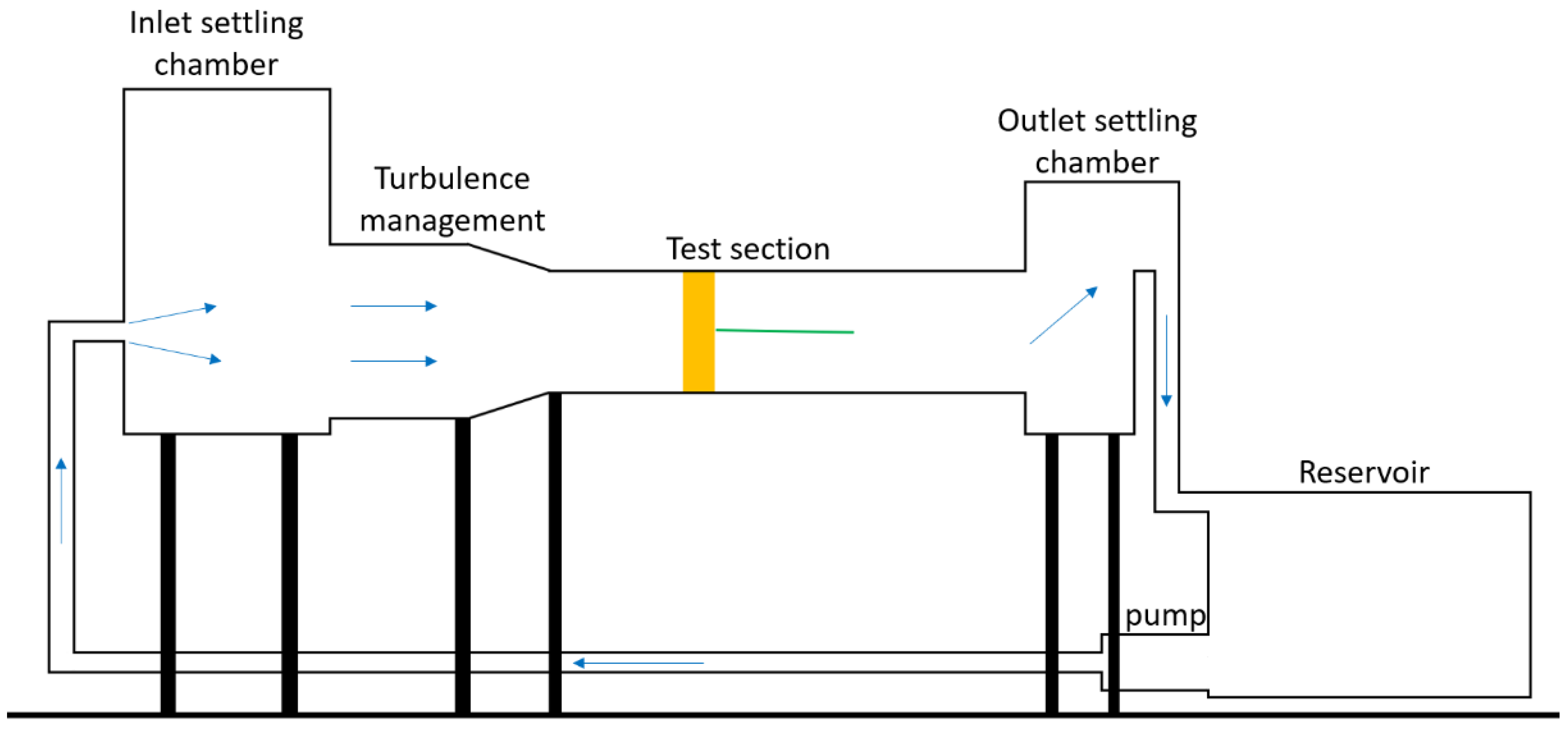
The demonstration and validation of the LSEVR technique will be carried out on measurements taken downstream of a cylinder mounted in cross-flow. A single 1” (25.4 mm) diameter brass cylinder was placed in an experimental water flow tunnel, arranged as depicted in
Figure 1. The working section was 0.3 m × 0.37 m and the cylinder was spanned the full height of the working section. Further details of the tunnel may be found in [
27].
Two-component PIV measurements were carried out on a plane at half-height of the working section (0.15 m) and covered a region of approximately 0.12 m × 0.12 m immediately downstream of the cylinder. Illumination was provided by a New Wave Pegasus 527 nm laser operating at 1 kHz with 10 mJ/pulse. Images were acquired using a Photron APX 1MP camera (Photron, Tokyo, Japan). Timing and synchronisation of the components were controlled using LaVision PTU 8 and DaVis v7 software. Calculation of the PIV vector fields was carried out within the DaVis software using multi-pass, reducing interrogation region. A single initial pass at 64 × 64, 50% overlap was followed by two passes at 32 × 32, 50% overlap. The final vector spatial resolution of 1.905 mm × 1.905 mm and temporal resolution of 1 kHz.
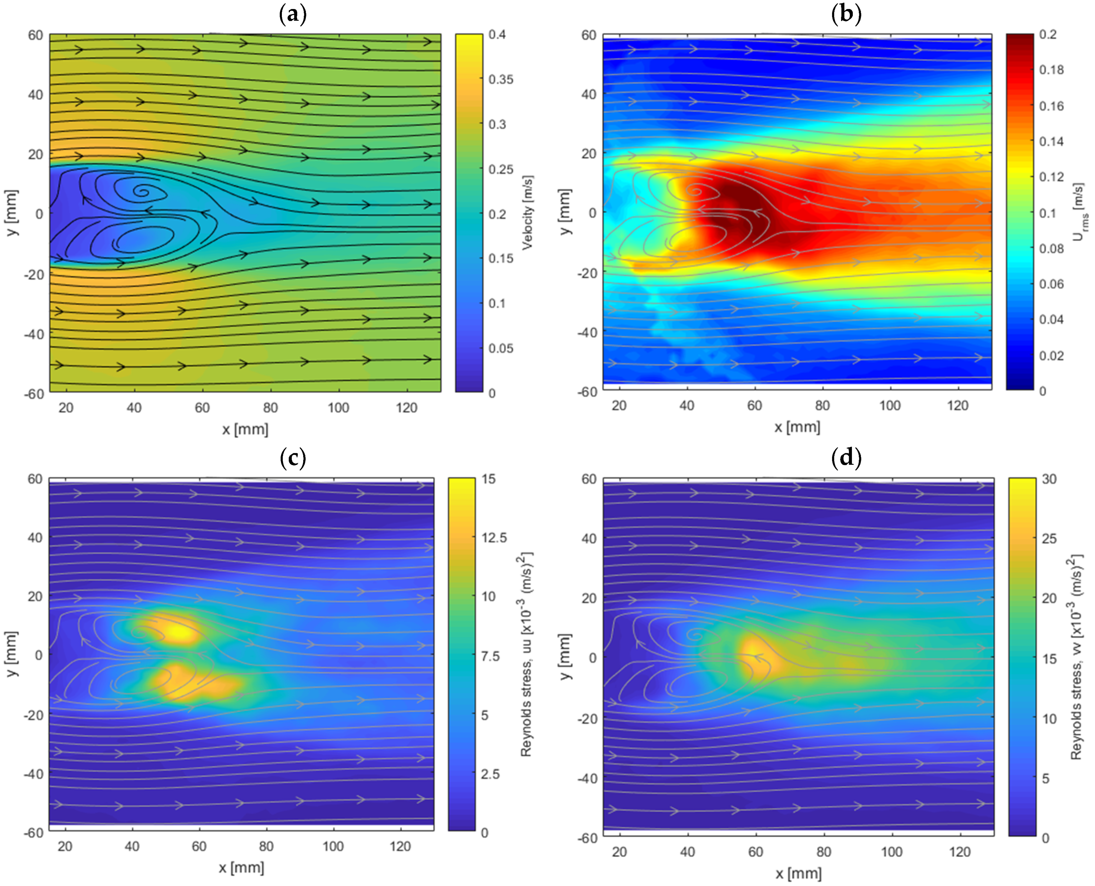
A total of 3072 vector fields were calculated and a summary of the flow fields is provided in
Figure 2. The ensemble average (
Figure 2a), velocity RMS (
Figure 2b) and Reynolds stresses (
Figure 2c,d) exhibit the well-known downstream wake region and vortex shedding behaviour commonly reported for this flow case [
28,
29]. Considering the turbulent areas in which the vortex shedding is occurring, one would expect high spatial velocity gradients. It is in this condition where modelling of the velocity field (by interpolation or otherwise) for the purposes of vector replacement would be most challenging. Therefore, a point is selected in this region, approximately half-way downstream in the measured area as a site for analysis and demonstration of the LSEVR technique. It should be noted that it would be possible to demonstrate the technique elsewhere within the domain such as the free-stream region. However, in this region with high spatial uniformity, it is expected that linear interpolation techniques would be fully capable of performing well and should have a lower computational cost than the LSEVR technique.
3.3. Validation Point, VP1 Analysis
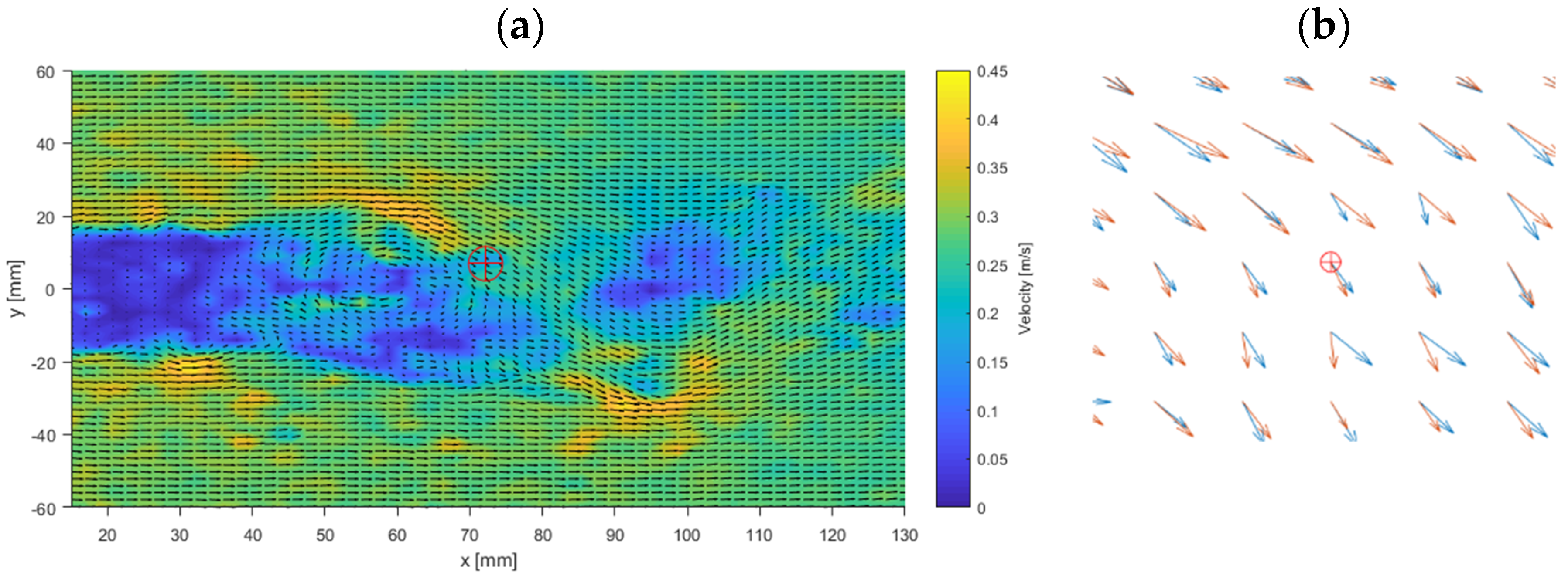
A validation point,
VP1 located at x = 72.14 mm, y = 6.90 mm is chosen as the site for demonstration and validation. It is important that this point be within the free-sheer layer and be exposed to turbulent vortex shedding in order to test the robustness of the technique. To demonstrate the nature of the turbulent flow, an example of an instantaneous velocity field (t
fr = 1) is presented in
Figure 3a with
VP1 marked. A zoomed view showing only the few surrounding vectors is presented in
Figure 3b where the unsteady nature is demonstrated by presentation of another timestep overlaid (t
fr = 10). Observing the differences between the two flow field time steps in
Figure 3b shows how due to an approaching eddy at that time, there is significant change in a few of the vectors surrounding
VP1. However,
VP1 itself does not change significantly. This illustrates the potential difficulties that need to be overcome by any vector replacement technique applied.
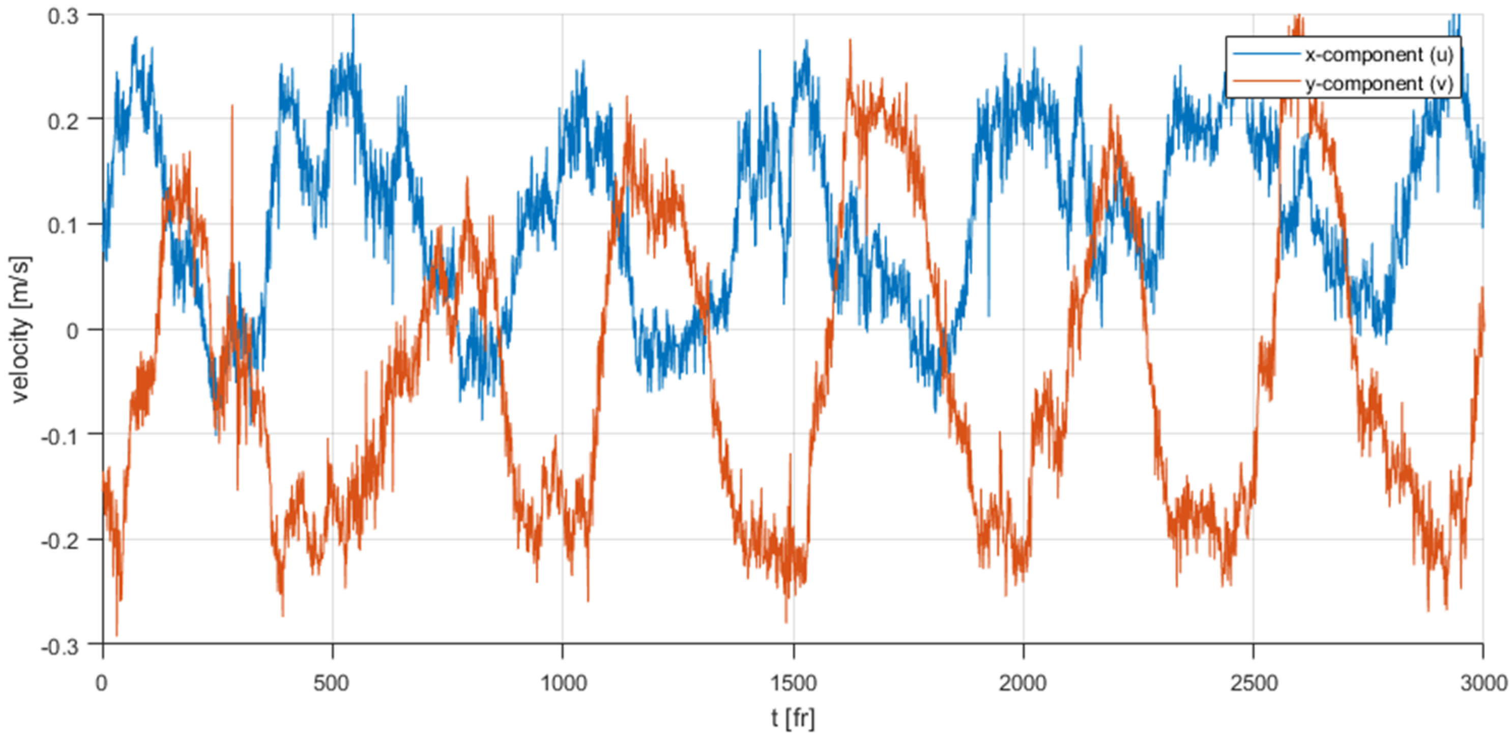
The true oscillatory nature of the flow in this region is not revealed so far, however by plotting the time history for
VP1 this is revealed in
Figure 4. A frequency related to the shedding of vortices in this region is revealed and evidence of turbulence is further exhibited. It is therefore recommended that the point
VP1 be considered as a worst case for application of the LSEVR technique.
In order to apply the technique, the vector data at VP1 will be removed from a number of time steps to emulate the situation requiring the replacement of a spurious vector. To clarify, this would be the situation once the vector has already been identified as spurious, removed and requires calculation of an estimate for replacement.
Firstly,
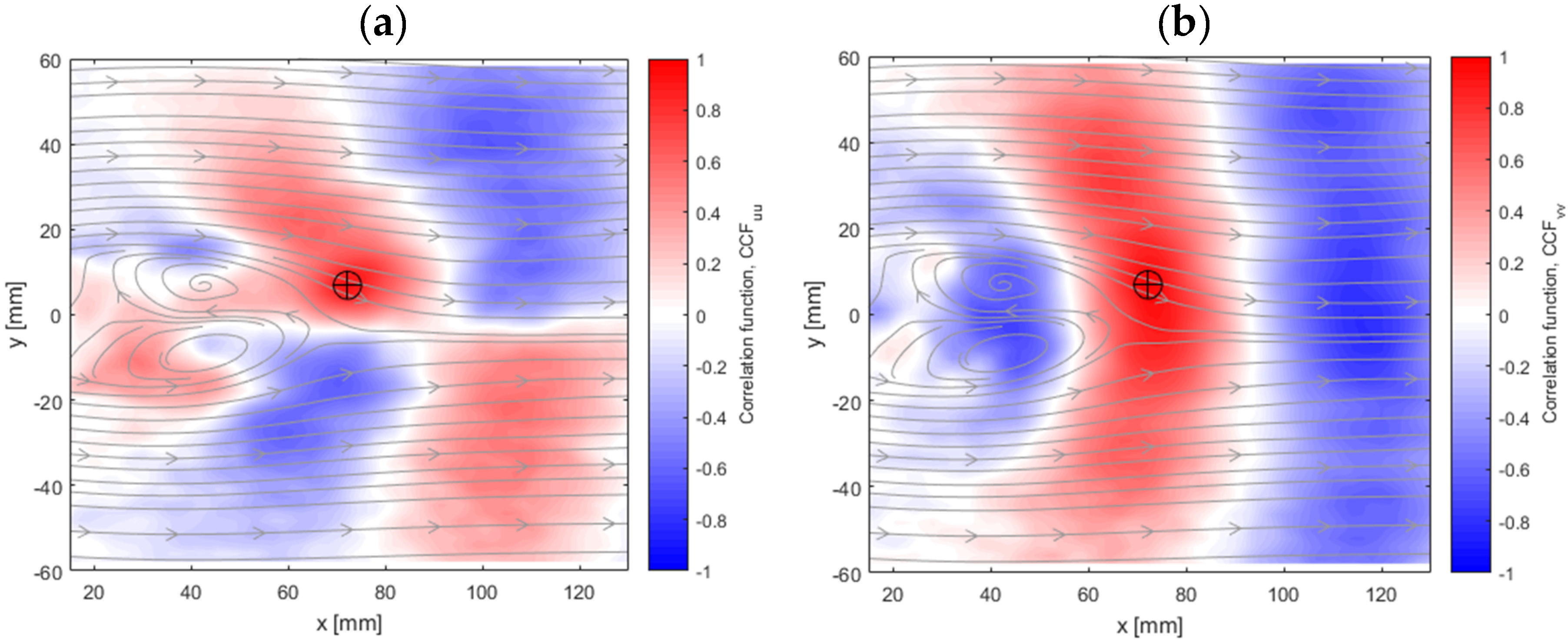
Figure 4 presents evidence that the site does regularly have valid, non-sparse data and therefore is suitable for LSEVR. Following this step, using valid time samples, the spatial correlation for each velocity component, in this case two-component, is calculated (according to Equation (3)) and presented in
Figure 5.
Before proceeding, there are some interesting observations about the flow revealed by
Figure 5. Firstly, the oscillatory nature is further evidenced in
Figure 5b which shows a vertical band of high-correlation with two adjacent highly negative correlations. Secondly, a chequerboard effect is exhibited in
Figure 5a.
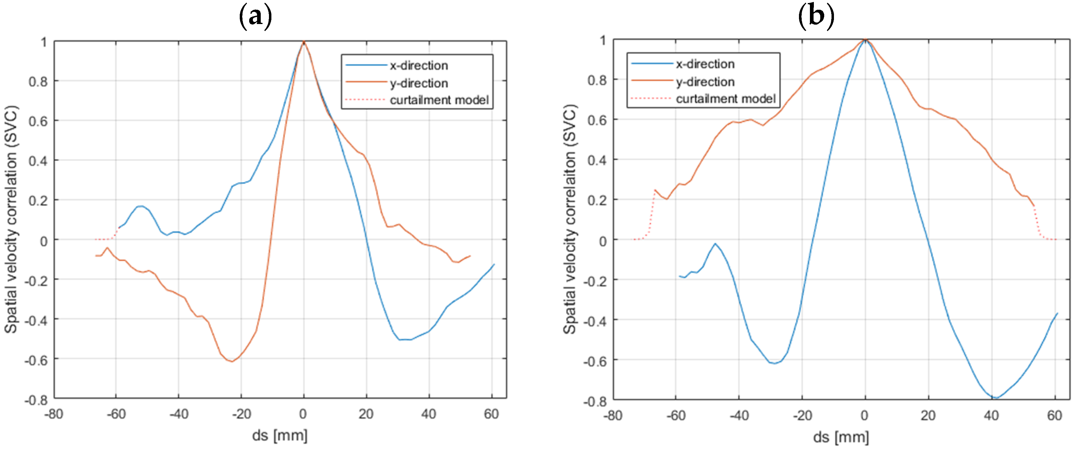
Taking straight-line profiles through
VP1 in
Figure 5 allows the spatial velocity correlation (SVC) for each component in each direction to be quantified and is presented in
Figure 6. Further, this allows for calculation of the integral length scales.
It should be noted that for this calculation, all profiles are required to have a zero-crossing by definition of integral length scale. Often in experimentally determined SVCs and therefore integral length scales, it is possible that there is no zero crossing. This may be the case when there is large correlation in one (or more) directions, the measurement region is not sufficient to capture all scales of flow structure or the point selected is close to an extremity of the measurement region. The former is demonstrated in
Figure 5b and subsequently
Figure 6b. It can be observed that a highly anisotropic correlation exists in the y-component of velocity. Hollis discusses how this may be overcome with a curtailment model, Equation (5), where subscript
c denotes the value at curtailed point [
30]. Hollis discusses several approaches to modelling the curtailment and the impact on obtained length scales. However, for the purposes of the calculation here, it is desired that a robust method be used that is suitable for many areas within the flow, and whilst Equation (5) may effect the absolute obtained length scale, it would not significantly impact on the selection of sensors and subsequent LSEVR calculation.
The length-scales may be calculated in all directions for all components. A summary of the resulting length scales is presented in
Table 1. Firstly, it should be noted that all but the aforementioned y-direction, y-component velocity have a length scale of approximately 10 mm. This value should be carefully considered when selecting the region in which sensors should be selected. It is therefore determined that the points to be selected as sensors for the LSEVR should be within 10 mm of
VP1 to maximise LSEVR effectiveness. Given the vector grid resolution of 1.90 mm × 1.90 mm, a region of no greater than 5 × 5 should be considered. Again, it could be noted that the region need not be square, and the anisotropy of the correlations could be considered if required; however, that is not the case here.
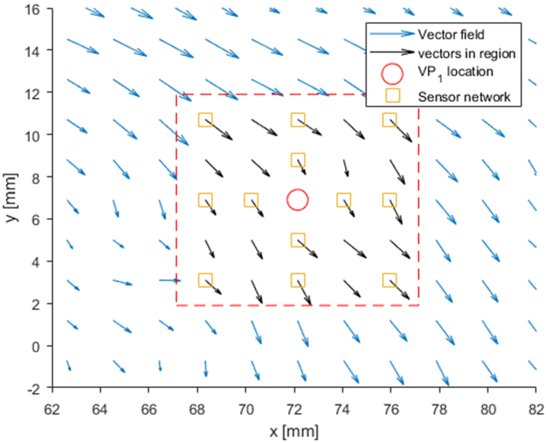
The next step of the procedure requires a sensor network to be distributed around the site (
VP1) to calculate the ‘
a’ matrix and allow subsequent estimation of the missing vector at
VP1. It is suggested that for accuracy of 75%, then at least 7 sensors should be used [
24]. However, it should be noted in that work by Butcher, the points were distributed randomly around the domain with no optimisation or effects of proximity to the point to be estimated exploited. It is expected in this application, a greater accuracy may be achieved due to the previous step of identifying highly correlated regions. Nonetheless, these values may serve as an upper limit to the number of points that should be required.
Within the defined limits and within the indicated region, a network of sensors is distributed as depicted in
Figure 7. Sensors are selected along the lines of the profiles represented in
Figure 6 with an additional point at each corner of the region giving a total of 12 sensors.
The next step involves the calculation of the ‘
a’ matrix over a number of time-step in which valid data exists. For this exercise, 100 randomly selected instances; from the 3072 available, shall have the vector at
VP1 deleted in order to emulate a removed spurious vector. This is achieved using random permutation function in Matlab for 1–3072 to generate frame number. For each condition, a symmetrical temporal window with the span of 100 time-steps shall be used to generate the ‘
a’ matrix. It should be noted that while 100 is used nominally (±50 excluding t), in the case where any of the time steps contain erroneous data, or t < 51 (i.e., there are less than 50 preceding time steps available), there may be less than 100 frames used as inputs to Equation (1). This approach is selected to improve efficiency of LSEVR by not carrying out the calculation unnecessarily. Further, given the periodic nature demonstrated in
Figure 4, the approach could lead to improved performance by selecting only data in the temporal vicinity of the vector to be estimated. For brevity, only the steps for the first randomly selected timestep are presented (t = 2503), however all further analysis and performance evaluation will be carried out on the full set of 100 estimations.
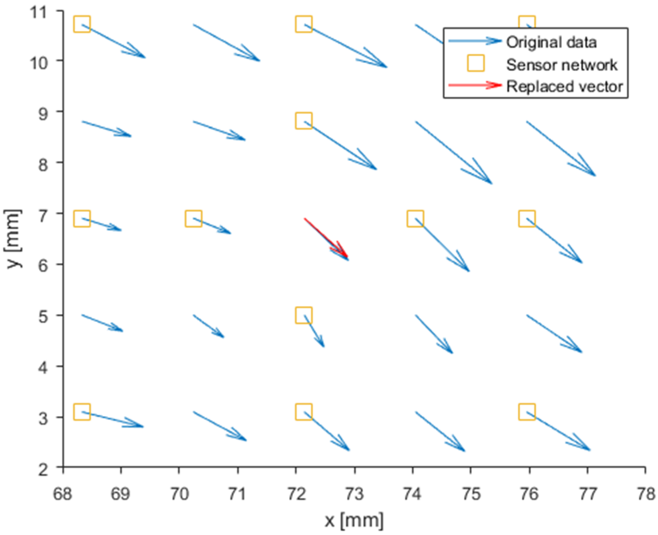
For the test case to be presented, t = 2503, the velocity component values at sensor location at t = 2453 to 2502 and 2504 to 2553 are extracted and used together with the
VP1 values to generate the ‘
a’ matrix according to Equation (1). Then, only the sensor values at t = 2503 are used with the ‘
a’ matrix and Equation (2) to produce the estimate of vector at
VP1 at t = 2503. This is plotted together with the original data for comparison in
Figure 8. The plot reveals a high similarity of the replacement vector with the original data set. It should be emphasised that while the original vector at
VP1, t = 2503 was known, it was not used in the calculation of the ‘
a’ matrix nor in the estimation. The purpose of retaining the value at this point was to provide a direct comparison to replacement for validation purposes.
3.4. Performance Relative to Other Approaches
To fully test the effectiveness of LSEVR, it shall be compared to other common techniques of data replacement. For this purpose, 2 techniques of interpolation shall be considered: bilinear and bicubic, both of which will be implemented using Matlab and only the values at sensor locations for the applicable time step. Similar to the previous demonstration, the comparison will be presented for a single time, t = 2503, but performance shall be assessed and summarised based on applying the technique to the 100 test cases randomly selected from all time steps.
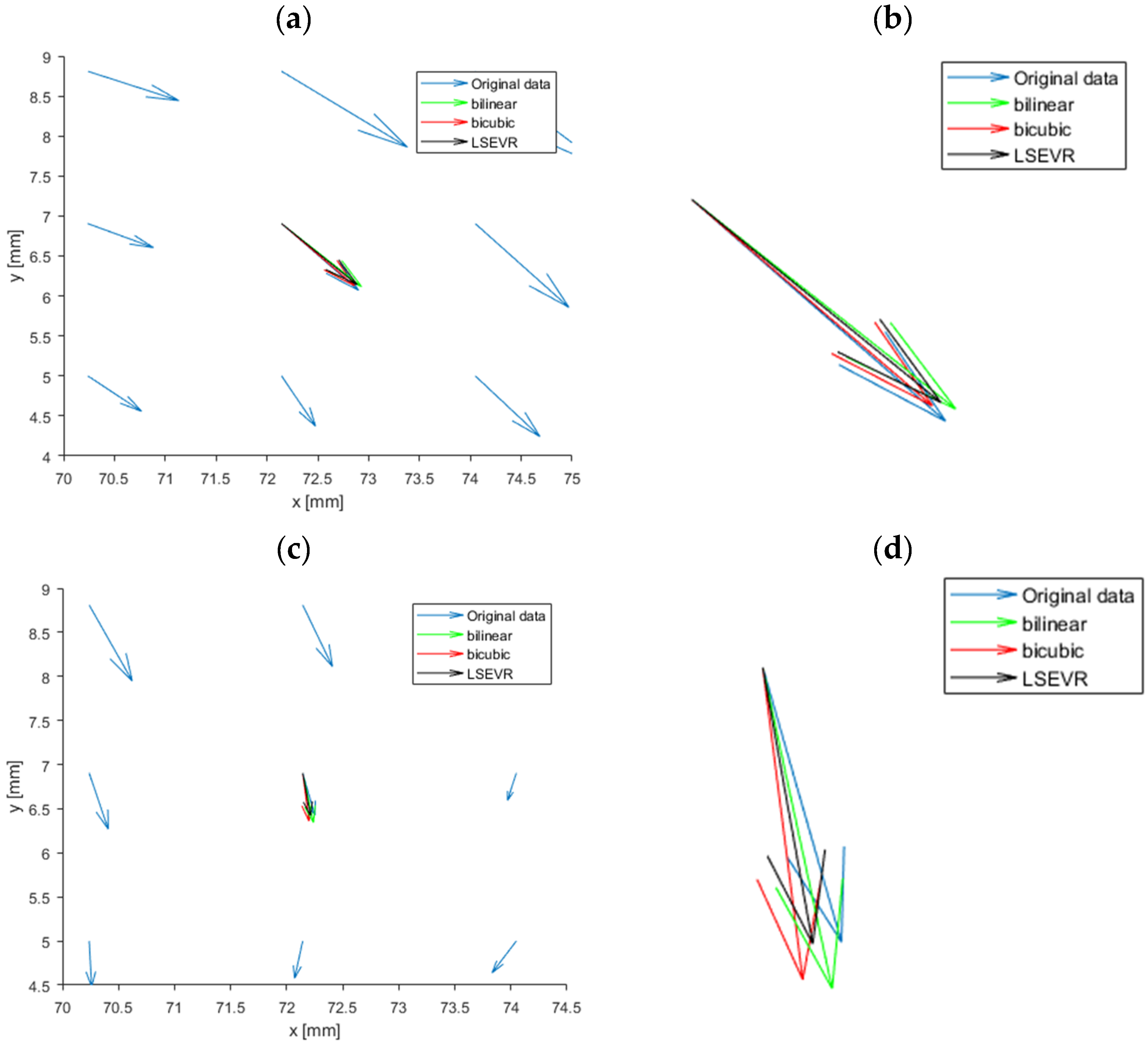
A direct comparison to bilinear and bicubic interpolation for the time step t = 2503 is presented in
Figure 9a with a zoomed view of the replaced vector in
Figure 9b. It can be deduced that in this particular situation, there is minimal difference between the replacement methods with bicubic interpolation performing marginally better, however it is reasonable in this case that either bicubic or LSEVR would be suitable. The similarity of performance may be attributed to smaller velocity gradients within the immediate vicinity at this time instance. Analysing the next randomly selected timestep, t = 2782 reveals a condition with increased velocity gradients.
Figure 9c,d present the estimations and zoomed views respectively. In this condition, there is some difference between the estimations. The magnitude for both bilinear and bicubic are overestimated while the LSEVR magnitude is closer to the original data. However, all show some difference in the vector direction. It is expected that with further increases in velocity gradient the disparity between the interpolation methods and LSEVR may increase.
Further to the two presented conditions, the vectors at
VP1 are estimated for the remaining 98 of 100 randomly selected test conditions. For each time condition, the error is calculated according to Equation (6), where
Uoriginal refers to the original velocity at
VP1 for that timestep, i.e., the value that should be estimated.
Equation (6) is evaluated across all timesteps and for each of the three replacement methods independently.
Table 2 summarises the resulting performance metrics for each method. Firstly, there is compelling evidence that on average the LSEVR technique outperforms both bilinear and bicubic interpolation techniques over the range tested. It should be noted that a region was purposefully selected in the flow in which reconstruction techniques would typically suffer, and this is evident in the average errors. Further, analysis of the results revealed that many of the high errors from all three techniques occur when the real velocity magnitude at
VP1 is close to zero. If the low velocity conditions are disregarded, the percentage errors for all techniques reduce to 13.03%, 10.62% and 7.12% for bilinear, bicubic and LSEVR respectively.
The number of instances in which there is greater than 10% error is also reduced using the LSEVR technique in comparison to the two interpolation methods which themselves rank as expected. However, the cost of LSEVR is increased computational expense. It has been shown how the computation time for ‘
a’ matrix generation in proportional to the square of the number of sensors [
24]. It would therefore be possible to reduce the cost by reducing number of sensors at potential expense of increased estimation error.
3.5. Further Validation Points, VP2 and VP3
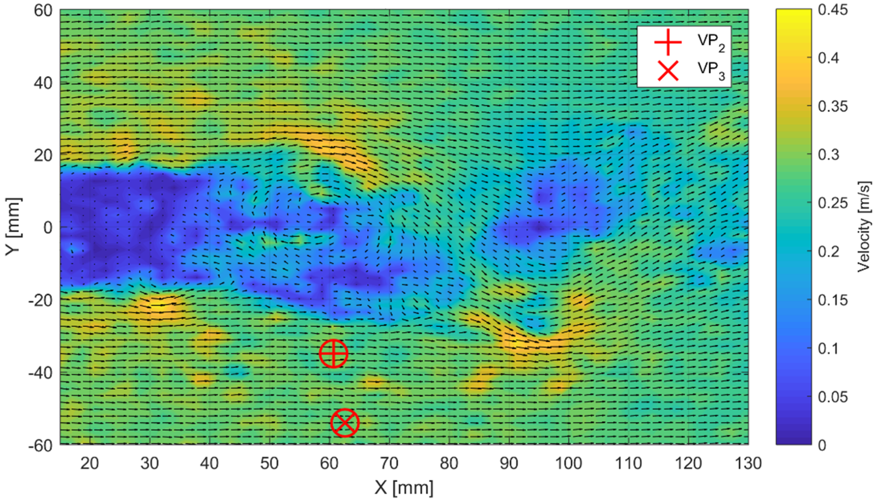
The previous section has demonstrated the ability of LSEVR in an area which would typically be problematic for interpolation-based techniques due to the high velocity gradients present in a turbulent, free-shear region. For completeness, this section will apply LSEVR within the free-stream area, comparing the relative performance against bilinear and bicubic interpolation. The points selected,
VP2 and
VP3 are presented in
Figure 10.
For each of the two additional test points, the process set out in
Section 3.3 and
Section 3.4 have been followed, with the additional bounding of the wall proximity of
VP3. This has resulted in the same sensor configuration style as that applied to
VP1. For brevity, equivalent cross-correlation plots for each of these points is not presented here as this is described in detail for
VP1. The resulting error for
VP2 and
VP3 are presented in
Table 3.
There are a few observations to note about the performance and relative performance of each of the replacement techniques for each VP2 and VP3. Firstly, all techniques for both points perform better than was the case for VP1 due to smaller velocity gradients in the case of interpolation and fewer significant velocity fluctuations in the case of LSEVR. Of the two points, VP3 is closer to free-stream behavior, and each technique performs well. In this situation, it could be beneficial to perform interpolation rather than LSEVR, due to the reduction in computational requirement with little benefit gained from LSEVR in this situation.
3.6. Regions with Multiple Removed Vectors
It was shown in the previous section how the performance of LSEVR produced more accurate replacement vectors than the bilinear and bicubic techniques over a range of tests conducted in a turbulent region of flow for a single removed vector. The condition in which LSEVR offers a more significant advantage is when multiple vectors in close proximity have been removed. This can commonly occur in experimental measurements, for example inhomogeneity in seeding creating sparse or overly-dense regions can affect multiple interrogation regions (in the case of PIV) for example and therefore vector locations.
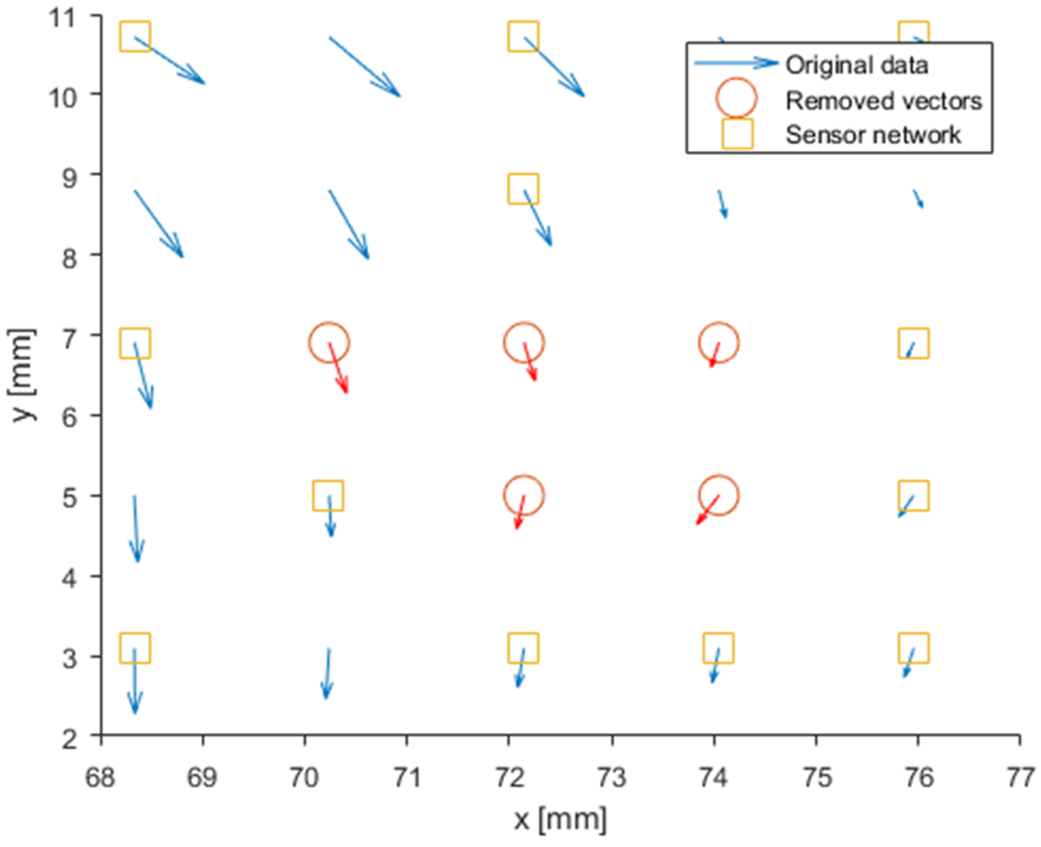
Interpolation methods rely on information from the nearest neighbours to estimate gradient and therefore value at the missing location. The LSEVR technique allows freedom to distribute the sensor network freely within the defined region. Considering the vector field partially presented in
Figure 9c (t = 2782), multiple vectors may be removed. These removed vectors and reconfigured sensor network are presented in
Figure 11.
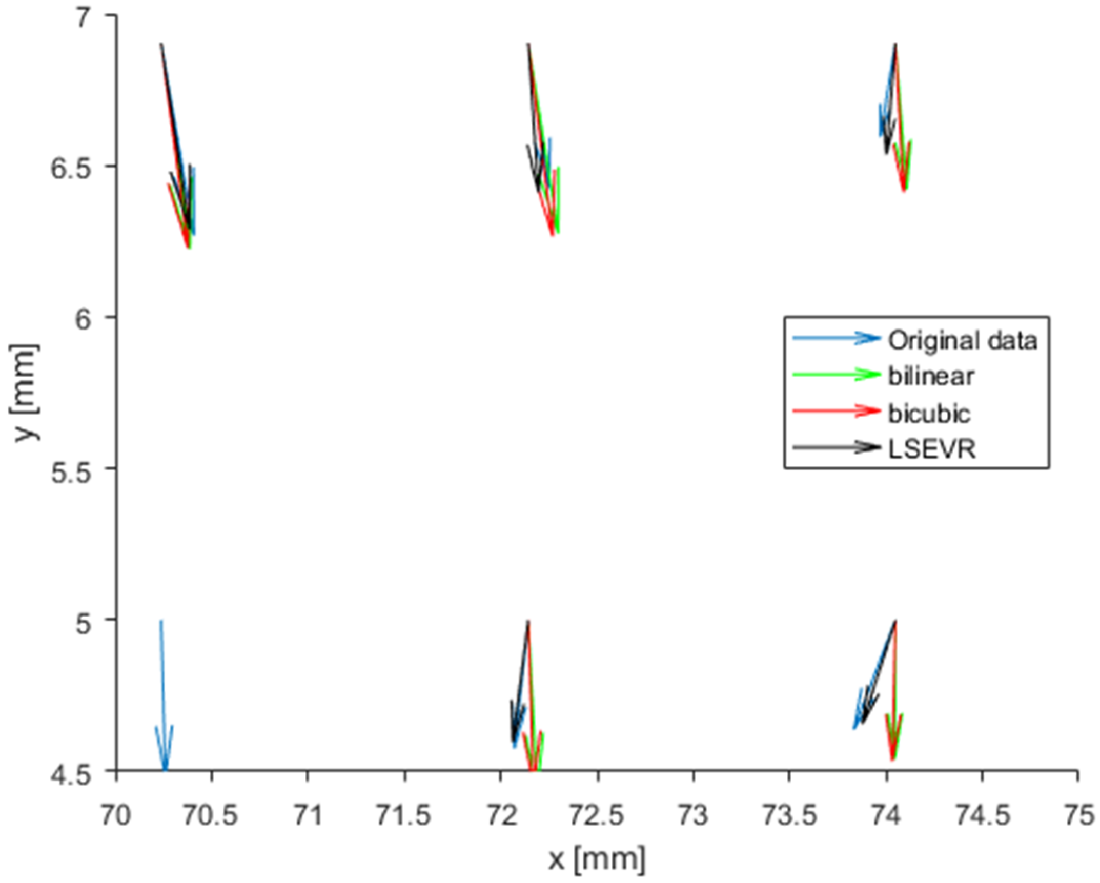
The resulting replacement vectors are compared in
Figure 12. For all but one vector replacement, the LSEVR technique produces a visibly closer representation of the originally removed vector. Further, its accuracy does not appear impacted for any one vector in comparison to another, evidence of the insensitivity to velocity gradient. In general, the bilinear and bicubic methods offer similar vectors, but both are significantly different to the LSEVR vector and original data.
The error at each vector position is calculated in the same manner as previous discussed and the results are summarised in
Table 4. It should be noted that all of the technique performed well for the vector located at x = 70.2 mm, y = 6.9 mm with errors of 7.33%, 8.06% and 4.61% for bilinear, bicubic and LSEVR respectively. This has contributed to a lower average error than was stated in
Table 2 for LSEVR, but in general the average is representative of the approximate error expected. Certainly, the two interpolation methods may suffer up to 55–70% error in the worst case; the two lower vectors in
Figure 12.
Applying the same approach of using 100 randomly selected timesteps, statistics are calculated the three approaches and compared in
Table 4. Here, the error is broken down to the error angle, that is the angle between the original vector and the replacement vector, and the error in magnitude (as %). This further reveals how errors manifest in each technique. It can be seen that each technique performs satisfactorily in estimating the vector magnitude, with LSEVR proving the most accurate. However, when the vector angle is considered, the two interpolation methods are significantly less representative than the LSEVR approach. This is visibly evident in the example provided in
Figure 11 where whilst some error in magnitude is just visible, the LSEVR angle is well estimated.
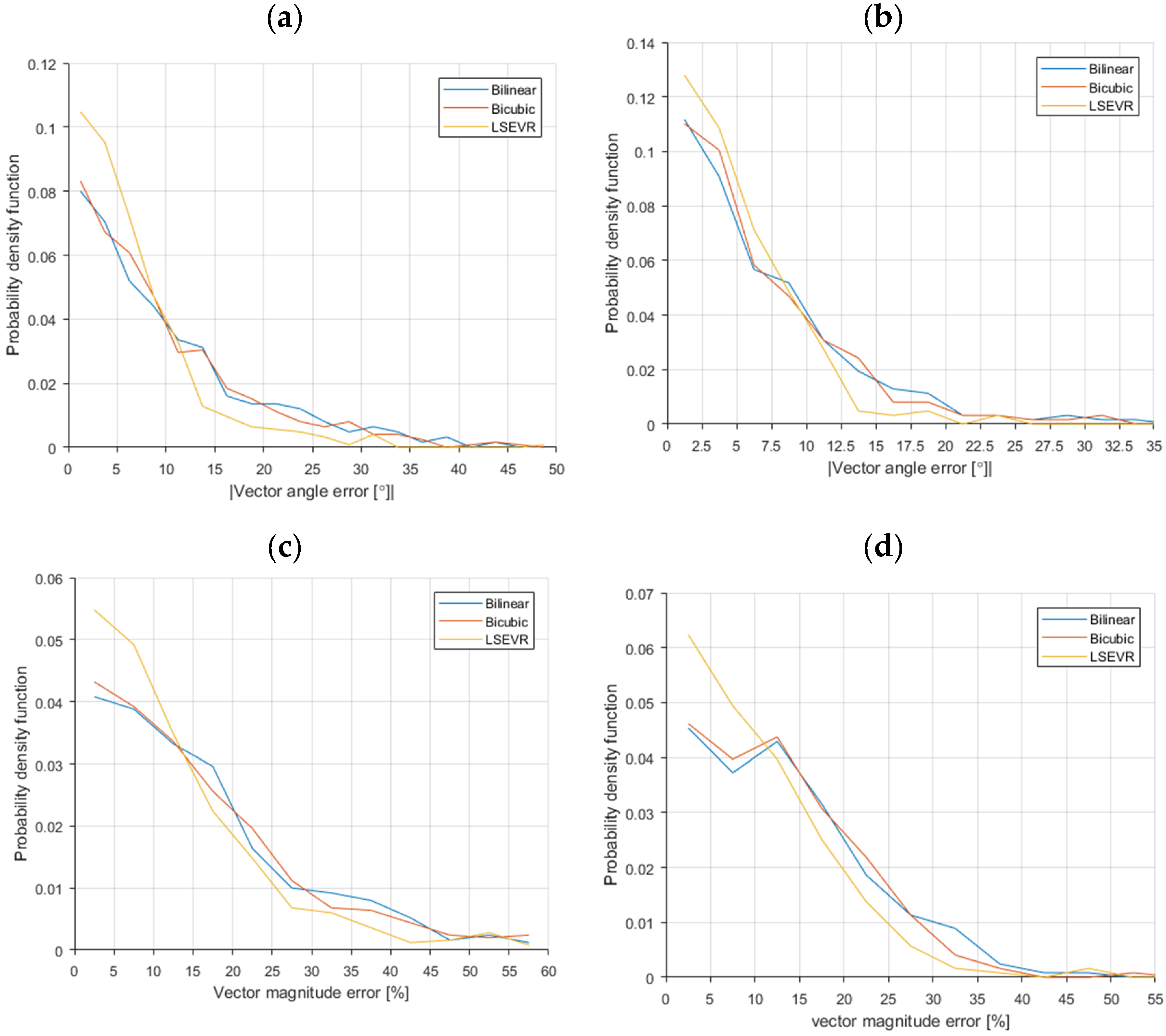
In addition to the average values presented in
Table 4, it is useful to consider the distribution of the errors associated with each of the three techniques in the form of probability density functions (PDFs), presented in
Figure 13. This is calculated on all five vectors to be replaced in the clumped sparse region (according to
Figure 11) over 100 time-steps, i.e., 500 total vectors for each technique.
Considering
Figure 13a,c, the vector angle and magnitude errors respectively, the LSEVR technique provides a significant reduction in error of the replacement vector. In terms of the vector error angle there are far fewer occurrences of high angle error in comparison to the other two techniques. When considering the error in vector magnitude, the advantage is less significant, however the LSEVR offers a clear advantage.
It is in this condition, when there are multiple adjacent or blocks of vectors that the LSEVR is most useful. Here, interpolation techniques have been shown to perform poorly, particularly in the estimation of vector angle.
Throughout the examples and values presented thus far, it has been discussed how close to zero values for the vector to be replaced can result in a disproportionally large error across all three techniques. Therefore, an additional two PDFs are presented in
Figure 13b,d which are based only on data with a greater (original) magnitude of 0.1 ms
−1. As one may expect, all three techniques show reduced error.
A noteworthy observation from this part of the study is that due to the independent application of LSE equations for each vector to be replaced, the technique is readily adapted for parallelisation which was the case here. The result is that there was no significant increase in computational time to replace five vectors rather than one (considering wall time not CPU time), providing there are the necessary computational provisions available.
4. Conclusions
In the experimental determination of velocity fields, there are myriad potential causes of erroneous vectors. These may present themselves either as clumps or regions of sparse vectors, individual erroneous vectors or a combination within the measurement volume. The erroneous regions may be persistent or instantaneously occurring. Much research effort has been carried out particularly in the field of PIV analysis to detect and replace these problematic vectors.
The presented work introduces the use of LSE as a vector replacement methodology LSEVR, highlighting advantages over commonly employed techniques and discussing the limitations and drawbacks. A five-step explanation of the technique is presented with suggestions of when the steps can be missed and the process streamlined, notably when there is more flow information known a priori. Two-point statistics, specifically the spatial velocity correlation function is utilised to identify a suitable region size for selection of the sensor network.
To demonstrate and test LSEVR, an experimental PIV data set is used of a commonly studied flow case of a single, stationary cylinder in cross-flow. From the complete dataset, a point is identified in the most turbulent region, the free-sheer layer. Analysis presented about this point, VP1 shows there is vortex shedding and some oscillatory behaviour of the flow velocities. Vector replacement at 100 randomly selected time steps is carried out alongside bilinear and bicubic interpolation for comparison.
In the majority of conditions, the LSEVR methodology performed better than both interpolation approaches but with increased computational cost. Typically, the LSEVR was shown to have a reduced error of 3–6%. The performance of all techniques may be acceptable and interpolation methods are widely used for this purpose. This is particularly the case if the spatial resolution of the experiment allows multiple vectors to represent flow structures.
To further demonstrate the robustness of the technique, two further points in the flow fields with significantly different characteristics were chosen to evaluate the relative performance. Points in the free stream were reasonably well estimated by both interpolation techniques and slightly better by LSEVR. In these conditions, where interpolation typically performs well, it may be more efficient to interpolate, applying LSEVR in areas where interpolation would suffer accuracy loss.
However, the strength of the technique lies in the cases with multiple sparse or removed spurious vectors in close proximity or clumps. In this condition, interpolation methods performed poorly with errors in the region of 40%+ while LSVR exhibited significantly reduced errors of approximately 10% with no detrimental impact identified when the sensor network requires reconfiguration. Further, due to the LSE equations being applied independently for each required vector replacement, the technique can readily be parallelised as was the case here. The result was no discernible increase in wall time calculation for the five replacements in comparison to a single replacement. This will depend on the configuration of the processing machine.
Finally, it was considered throughout this work that an adapted LSEVR routine could be implemented to detect spurious vectors as well as estimating a replacement. However, the increase in computational requirements would be too great if LSEVR were applied at every spatial and temporal data point in the flow. Therefore, it could be incorporated once a median test has identified a potential spurious vector, LSEVR could provide a comparative vector to use rather than a vector based on the standard deviation of neighbours as is often the case.


