Semi-Analytical Solutions for the Poiseuille–Couette Flow of a Generalised Phan-Thien–Tanner Fluid

Abstract

This work presents new analytical and semi-analytical solutions for the pure Couette and Poiseuille–Couette flows, described by the recently proposed (Ferrás et al., A Generalised Phan-Thien–Tanner Model, JNNFM 2019) viscoelastic model, known as the generalised Phan-Thien–Tanner constitutive equation. This generalised version considers the Mittag–Leffler function instead of the classical linear or exponential functions of the trace of the stress tensor, and provides one or two new fitting constants in order to achieve additional fitting flexibility. The analytical solutions derived in this work allow a better understanding of the model, and therefore contribute to improve the modelling of complex materials, and will provide an interesting challenge to computational rheologists, to benchmarking and to code verification.

1. Introduction

It is well known that much can be learned about a physical phenomenon if a mathematical model exists that can mimic and predict its behavior. The world of complex fluids is no different, and, therefore, several models have been proposed over the years for that purpose. These models can be more or less complex, depending on the properties of the fluids that are taken into account.

In this work, we are interested in viscoelastic materials [1], for which several models have been proposed in the past. One can classify these models as: differential (that make use of the local deformation field only) and integral (that take into account all the past deformation at each instant). Differential models usually allow a faster numerical solution of the differential equations involved, while integral models are computationally expensive and may lead to error propagation. On the other hand, integral models allow a better modelling, since they incorporate the real world fluid memory (the present state is influenced by all past weighted deformations). It is therefore of major importance to improve the fitting capabilities of differential models and reduce the computational effort needed to compute integral models.

In a recent work, Ferrás et al. [2] proposed an improved differential model based on the model by Nhan Phan-Thien and Roger Tanner (PTT [3]), derived from the Lodge–Yamamoto type of network theory for polymeric fluids. The constitutive equation proposed by Nhan Phan-Thien and Roger Tanner, for the case of an isothermal flow, is given by:

$$f\left({\tau }_{kk}\right)\mathbf{\tau }+\lambda \mathring{\mathbf{\tau }}=2{\eta }_p\mathbf{D}$$

(1)

with

$$f\left({\tau }_{kk}\right)=1+\frac{\epsilon \lambda }{{\eta }_p}{\tau }_{kk},$$

(2)

where $\mathbf{D}$ is the rate of deformation tensor, $\mathbf{\tau }$ is the stress tensor, $\lambda$ is a relaxation time, ${\eta }_p$ is the polymeric viscosity, ${\tau }_{kk}$ is the trace of the stress tensor, $\epsilon$ represents the extensibility parameter and $\mathring{\mathbf{\tau }}$ represents the Gordon–Schowalter derivative defined as

$$\mathring{\mathbf{\tau }}=\frac{\partial \mathbf{\tau }}{\partial t}+\mathbf{u}·\nabla \mathbf{\tau }-{\left(\nabla \mathbf{u}\right)}^T·\mathbf{\tau }-\mathbf{\tau }·\left(\nabla \mathbf{u}\right)+\xi \left(\mathbf{\tau }·\mathbf{D}+\mathbf{D}·\mathbf{\tau }\right).$$

(3)

Here, $\mathbf{u}$ is the velocity vector, $\nabla \mathbf{u}$ is the velocity gradient and the parameter $\xi$ accounts for the slip between the molecular network and the continuous medium (it should be remarked that for the derivation of the analytical solutions we will consider $\xi =0$). Later, Phan-Thien proposed a new model, based on an exponential function form [4] and showed that this new function would be quite adequate to represent the rate of destruction of junctions, but the parameter $\epsilon$ should be of the order 0.01. The function $f\left({\tau }_{kk}\right)$ is given by:

$$f\left({\tau }_{kk}\right)=\exp \left(\frac{\epsilon \lambda }{{\eta }_p}{\tau }_{kk}\right).$$

(4)

Ferrás et al. [2] considered a more general function for the rate of destruction of junctions, the Mittag–Leffler function where one or two fitting constants are included, in order to achieve additional fitting flexibility [2]. The Mittag–Leffler function is defined by,

$$E_{\alpha ,\beta }\left(z\right)=\sum _{k=0}^{\infty }\frac{z^k}{\Gamma \left(\alpha k+\beta \right)},$$

(5)

with $\alpha$, $\beta$ real and positive. When $\alpha =\beta =1$, the Mittag–Leffler [5] function reduces to the exponential function. When $\beta =1$, the original one-parameter Mittag–Leffler function, $E_{\alpha }$, is obtained. Thus, the new function of the trace of stress tensor (now denoted by $K(.)$ instead of $f(.)$, to distinguish from the classical cases) describing the network destruction of junctions is written as:

$$K\left({\tau }_{kk}\right)=\Gamma \left(\beta \right)E_{\alpha ,\beta }\left(\frac{\epsilon \lambda }{{\eta }_p}{\tau }_{kk}\right),$$

(6)

where $\Gamma$ is the Gamma function and the normalisation $\Gamma \left(\beta \right)$ is used to ensure that $K\left(0\right)=1$, for all choices of $\beta$.

The linear and the exponential model of the Phan-Thien–Tanner has been frequently used in the literature, and in fact Ferrás et al. [6] considered a new quadratic version of the PTT model, i.e., a second-order expansion of the exponential model given by:

$$f\left({\tau }_{kk}\right)=1+\frac{\epsilon \lambda }{{\eta }_p}{\tau }_{kk}+\frac{1}{2}{\left(\frac{\epsilon \lambda }{{\eta }_p}{\tau }_{kk}\right)}^2.$$

(7)

Here, we compare the generalised Phan-Thien–Tanner (gPTT), given by Equation (6), with the linear, the exponential and the quadratic versions of the PTT (Equations (2), (4) and (7), respectively).

To compare these models, we study the dimensionless material properties in steady shear flow of the three versions of the PTT model and compare them with the new gPTT model, considering different values of $\alpha$ and $\beta$.

The material functions can be obtained considering a steady-state Couette flow in the x-direction, $\mathbf{u}=\left(\dot{\gamma }y,0,0\right)$, where $\dot{\gamma }$ is the shear rate. For this flow, considering the parameter $\xi =0$, the constitutive Equation (1) reduces to:

$$\left\{\begin{array}{cc}\hfill K\left({\tau }_{kk}\right){\tau }_{xx}& =2\lambda \dot{\gamma }{\tau }_{xy}\hfill \\ \hfill K\left({\tau }_{kk}\right){\tau }_{xy}& ={\eta }_p\dot{\gamma }.\hfill \\ \hfill {\tau }_{yy}={\tau }_{zz}& ={\tau }_{xz}={\tau }_{yz}=0\hfill \end{array}\right.$$

(8)

From the system of Equation (8), ${\tau }_{kk}={\tau }_{xx}$ and applying some algebra in the first two equations, a relationship between the shear stress and the normal stress is found,

$${\tau }_{xx}=2\frac{\lambda }{{\eta }_p}{\tau }_{xy}^2.$$

(9)

We can also obtain the viscometric material functions: the steady shear viscosity, $\mu \left(\dot{\gamma }\right)$, the first normal stress difference coefficient, ${\Psi }_1\left(\dot{\gamma }\right)$, and the second normal stress difference coefficient, ${\Psi }_2\left(\dot{\gamma }\right)$, which are given by:

$$\mu \left(\dot{\gamma }\right)=\frac{{\tau }_{xy}}{\dot{\gamma }},$$

(10)

$${\Psi }_1\left(\dot{\gamma }\right)=\frac{{\tau }_{xx}-{\tau }_{xy}}{{\dot{\gamma }}^2},$$

(11)

$${\Psi }_2\left(\dot{\gamma }\right)=\frac{{\tau }_{yy}-{\tau }_{zz}}{{\dot{\gamma }}^2}.$$

(12)

As for other versions of the simplified PTT models for which $\xi =0$, the second normal stress coefficient is null, ${\Psi }_2\left(\dot{\gamma }\right)=0$, so, we only need to find $\mu \left(\dot{\gamma }\right)$ and ${\Psi }_1\left(\dot{\gamma }\right)$. Therefore, manipulating the second equation of the system of Equations (8) we get,

$${\tau }_{xy}=\frac{{\eta }_p\dot{\gamma }}{K\left({\tau }_{xx}\right)}.$$

(13)

The dimensionless expression for the steady shear viscosity becomes,

$$\frac{\mu \left(\dot{\gamma }\right)}{{\eta }_p}=\frac{{\tau }_{xy}}{{\eta }_p\dot{\gamma }}=\frac{1}{K\left({\tau }_{xx}\right)}$$

(14)

and the dimensionless first normal stress coefficient is given by,

$$\frac{{\Psi }_1\left(\dot{\gamma }\right)}{2{\eta }_p\lambda }=\frac{{\tau }_{xx}}{2{\eta }_p\lambda {\dot{\gamma }}^2}=\frac{1}{{\left[K\left({\tau }_{xx}\right)\right]}^2}.$$

(15)

In [6], it was shown that, for the linear PTT, the quadratic PTT and the exponential PTT, the dimensionless material functions depend on the generalised Deborah number, $\sqrt{\epsilon }\left(\lambda \dot{\gamma }\right)$. We show that the same happens for the gPTT model. To obtain the material function for the gPTT model, we need to solve the non-linear system of equations (Equation (8)), which can be written in terms of ${\tau }_{xx}$ in the non-linear form:

$$\frac{1}{2}K{\left({\tau }_{xx}\right)}^2\frac{\epsilon \lambda }{{\eta }_p}{\tau }_{xx}=\epsilon {\left(\lambda \dot{\gamma }\right)}^2.$$

(16)

Giving values to $\frac{\epsilon \lambda }{{\eta }_p}{\tau }_{xx}$, we can find $\sqrt{\epsilon }\left(\lambda \dot{\gamma }\right)$ using Equation (16). Then, the function $K\left({\tau }_{xx}\right)$ is directly calculated, allowing us to obtain the material functions given by Equations (14) and (15).

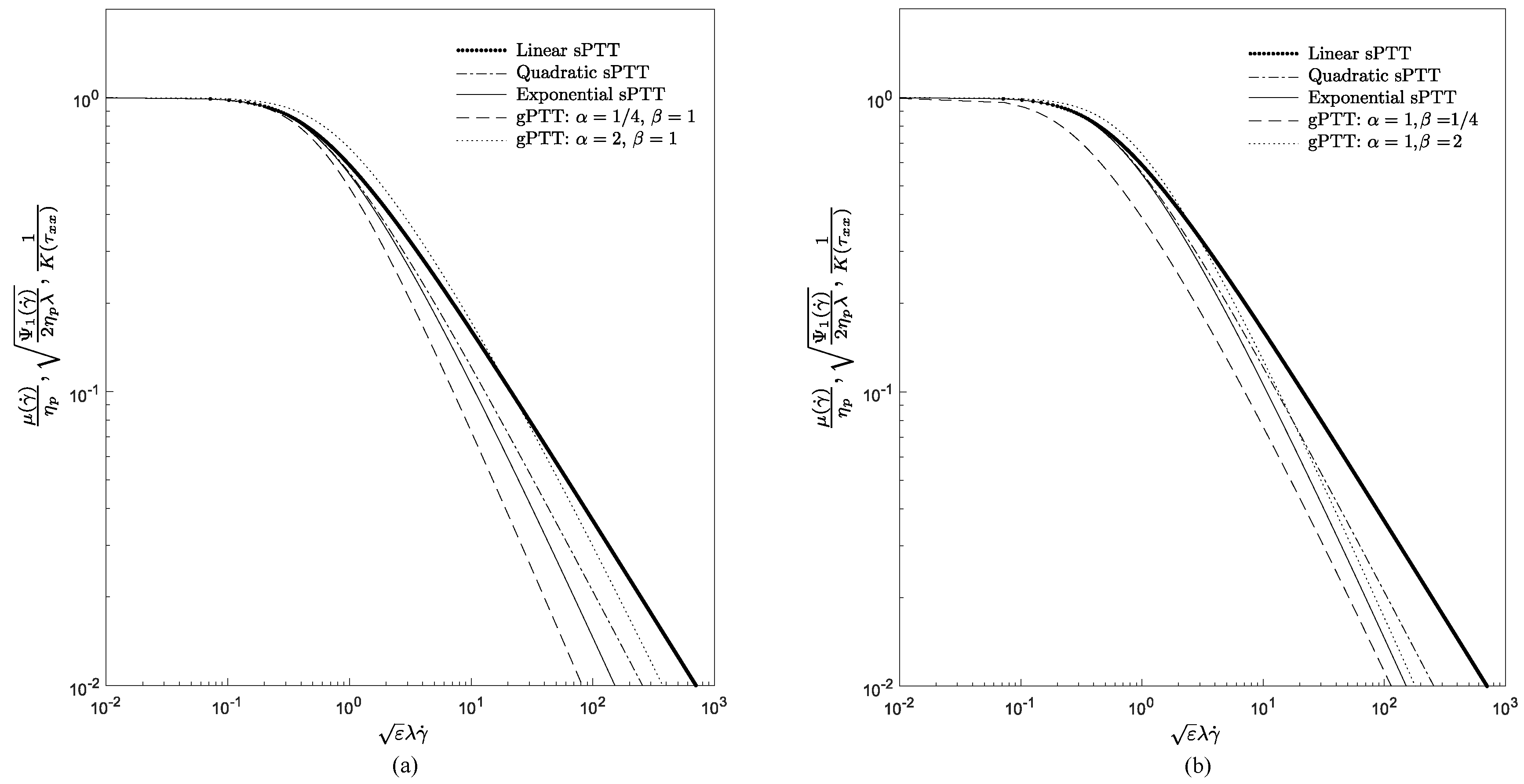
Figure 1 presents the dimensionless material properties for the steady-state Couette flow using three versions of the PTT (linear, quadratic, and exponential) and also the gPTT model. In Figure 1a, we set $\beta =1$ and use different values of $\alpha$, and, in Figure 1b, we set $\alpha =1$ and use different values to $\beta$.

We observe that the new generalised function allows a broader description of the thinning properties of the fluid. Both the thinning rate and the onset of the thinning behavior can be controlled by the new model parameters. Therefore, this new model must be further explored for weak flows, such as Couette flows.

This model was extensively studied for strong flows in [2], where an explanation on the influence of the new model parameters was provided.

Note that the exponential version of the model was developed to take into account the strong destruction of network junctions, which occurs, for example, in strong flows (e.g., extensional flows). Although the exponential model was derived for such strong flows, it was shown in [2] that the gPTT model could slightly improve the fitting for shear (weak) flows, considering polymer solutions. Here, we consider polymer melts.

Figure 2 shows that the gPTT model provides a much better fitting to weak flows of polymer melts (low density polyethylene melt [7]), even when using only one extra parameter ($\alpha$).

To quantify the error incurred during the fitting process, we used a mean square error given by

$${\displaystyle error=\sum _i^{N_{\mu }}{\left[log\mu {\left(\dot{\gamma }\right)}_i-log\mu {\left(\dot{\gamma }\right)}_{fi{t}_i}\right]}^2+\sum _j^{N_{{\Psi }_1}}{\left[log{\Psi }_1{\left(\dot{\gamma }\right)}_j-log{\Psi }_1{\left(\dot{\gamma }\right)}_{fi{t}_j}\right]}^2,}$$

(17)

$${\displaystyle erro{r}_{\mu }=\sum _i^{N_{\mu }}{\left[log\mu {\left(\dot{\gamma }\right)}_i-log\mu {\left(\dot{\gamma }\right)}_{fi{t}_i}\right]}^2,}$$

(18)

$${\displaystyle erro{r}_{{\Psi }_1}=\sum _j^{N_{{\Psi }_1}}{\left[log{\Psi }_1{\left(\dot{\gamma }\right)}_j-log{\Psi }_1{\left(\dot{\gamma }\right)}_{fi{t}_j}\right]}^2,}$$

(19)

with $N_{\mu }$ and $N_{{\Psi }_1}$ the number of experimental points obtained for $\mu \left(\dot{\gamma }\right)$ and ${\Psi }_1\left(\dot{\gamma }\right)$, respectively.

A better fit was obtained for the new generalised model when compared to the original exponential PTT model. The total mean square error obtained for the exponential PTT model was $29.7$, being five times the error obtained for its generalised version (for which a value of $6.0$ was obtained). The new model allows a better fit for low and high shear rates for the first normal stress difference (where the $erro{r}_{{\Psi }_1}$ obtained for the exponential PTT model is 20 times higher than the error obtained for the gPTT). For the shear viscosity, the gPTT model predicts a lower value (when compared to experimental data) for high shear rates (although it should be remarked that the $erro{r}_{\mu }$ is four times smaller when compared to the exponential model).

Based on what is described above, this work presents analytical and semi-analytical solutions for pure Couette and Poiseuille–Couette flows, described by the generalised Phan-Thien–Tanner constitutive equation. It is well known that the rate of destruction of junctions increases for strong flows (e.g., extensional flows), but, in this case, we consider weak flows, and study the capability of this new model to describe them. This is done by performing a parametric study for the influence of the gPTT parameters.

2. Analytical Solution for the gPTT Model in Couette flow

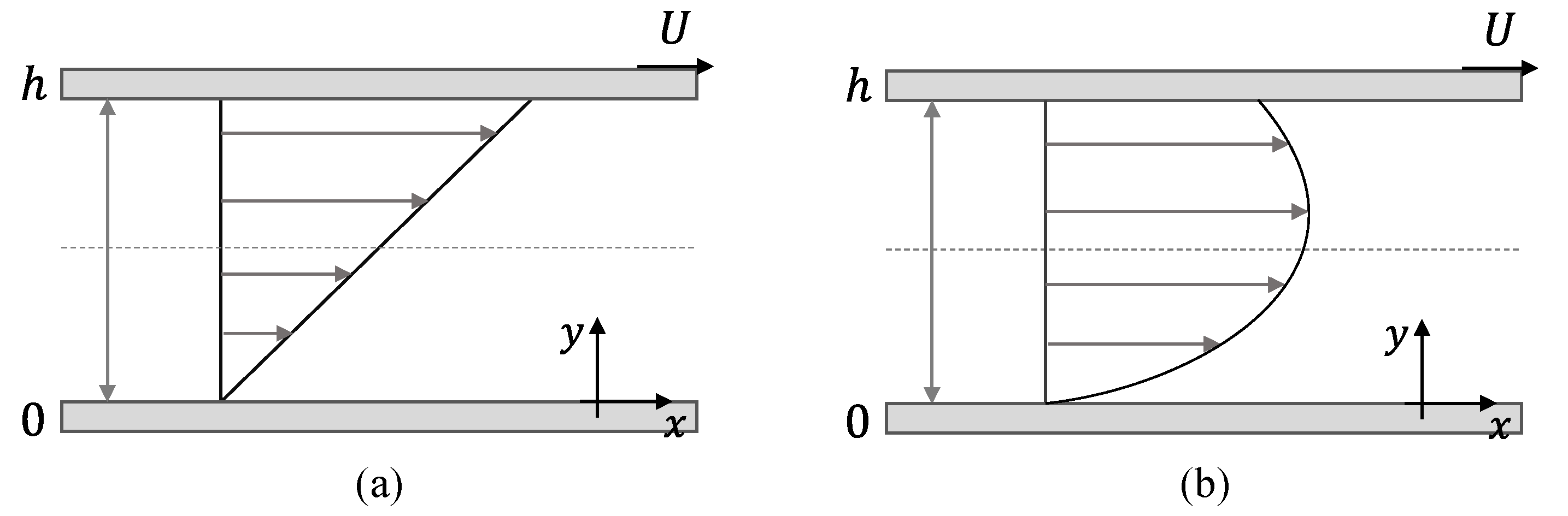
In this section, we derive the analytical solution for the fully developed flow of the gPTT model considering both Couette and Poiseuille–Couette flows (cf. Figure 3). To obtain closed form analytical solutions, the slip parameter in the Gordon–Schowalter derivative is set to $\xi =0$.

The equations governing the flow of an isothermal incompressible fluid are the continuity,

$$\nabla ·\mathbf{u}=0$$

(20)

and the momentum equation,

$$\rho \frac{D\mathbf{u}}{Dt}=-\nabla p+\nabla ·\mathbf{\tau }$$

(21)

together with the constitutive equation,

$$\Gamma \left(\beta \right)E_{\alpha ,\beta }\left(\frac{\epsilon \lambda }{{\eta }_p}{\tau }_{kk}\right)\mathbf{\tau }+\lambda \mathring{\mathbf{\tau }}=2{\eta }_p\mathbf{D},$$

(22)

where $\frac{D}{Dt}$ is the material derivative, p is the pressure, t is the time and $\rho$ is the fluid density.

We consider a Cartesian coordinate system with x, y, and z being the streamwise, transverse and spanwise directions, respectively. The flow is assumed to be fully-developed and therefore the governing equations can be further simplified since

$$\frac{\partial }{\partial x}=0\left(\mathrm{except}\mathrm{for}\mathrm{pressure}\right),\frac{\partial v}{\partial y}=0,\frac{\partial p}{\partial y}=0.$$

(23)

Therefore, Equation (21) can be integrated, leading to the following general equation for the shear stress:

$${\tau }_{xy}=P_{x}y+c_1,$$

(24)

where $P_x$ is the pressure gradient in the x direction, ${\tau }_{xy}$ is the shear stress and $c_1$ is a stress constant. This equation is valid regardless of the rheological constitutive equation. The constitutive equations for the generalised PTT model describing this flow can be further simplified leading to:

$$K\left({\tau }_{kk}\right){\tau }_{xx}=(2-\xi )\left(\lambda \dot{\gamma }\right){\tau }_{xy},$$

(25)

$$K\left({\tau }_{kk}\right){\tau }_{yy}=-\xi \left(\lambda \dot{\gamma }\right){\tau }_{xy},$$

(26)

$$K\left({\tau }_{kk}\right){\tau }_{xy}={\eta }_p\dot{\gamma }+(1-\frac{\xi }{2})\left(\lambda \dot{\gamma }\right){\tau }_{yy}-\frac{\xi }{2}\left(\lambda \dot{\gamma }\right){\tau }_{xx},$$

(27)

where the shear rate $\dot{\gamma }$ is a function of y ($\dot{\gamma }\left(y\right)\equiv \frac{du}{dy}$) and ${\tau }_{kk}={\tau }_{xx}+{\tau }_{yy}$ is the trace of the stress tensor. Assuming $\xi =0$, Equation (26) implies that ${\tau }_{yy}=0$, and the trace of the stress tensor becomes ${\tau }_{kk}={\tau }_{xx}$. Dividing Equation (25) by Equation (27), $K\left({\tau }_{xx}\right)$ cancels out, and we get the explicit relationship between the streamwise normal stress and the shear stress given by Equation (9).

Now, combining Equations (9), (24) and (27), the following shear rate profile is obtained,

$$\dot{\gamma }\left(y\right)=\Gamma \left(\beta \right)E_{\alpha ,\beta }\left(\frac{2\epsilon {\lambda }^2}{{\eta }_p^2}{\left(P_{x}y+c_1\right)}^2\right)\frac{\left(P_{x}y+c_1\right)}{{\eta }_p}.$$

(28)

The velocity profile can be obtained integrating the shear rate subject to the Couette boundary conditions (null velocity at the immobile wall),

$$u\left(0\right)=0$$

(29)

and an imposed constant velocity, U, at the moving wall,

$$u\left(h\right)=\mathrm{U}.$$

(30)

This leads to the following velocity profile:

$$u\left(y\right)=\mathrm{U}-\frac{\Gamma \left(\beta \right)}{{\eta }_p{P}_x}\sum _{k=0}^{\infty }\left({\left(\frac{2\epsilon {\lambda }^2}{{\eta }_p^2}\right)}^k\frac{{\left(P_{x}h+c_1\right)}^{2k+2}-{\left(P_{x}y+c_1\right)}^{2k+2}}{\Gamma (\alpha k+\beta )\left(2k+2\right)}\right),$$

(31)

where $c_1$ can be obtained by solving numerically the following equation,

$$\mathrm{U}=\frac{\Gamma \left(\beta \right)}{{\eta }_p{P}_x}\sum _{k=0}^{\infty }\left({\left(\frac{2\epsilon {\lambda }^2}{{\eta }_p^2}\right)}^k\frac{1}{\Gamma (\alpha k+\beta )}\frac{{\left(P_{x}h+c_1\right)}^{2k+2}-{c_1}^{2k+2}}{2k+2}\right).$$

(32)

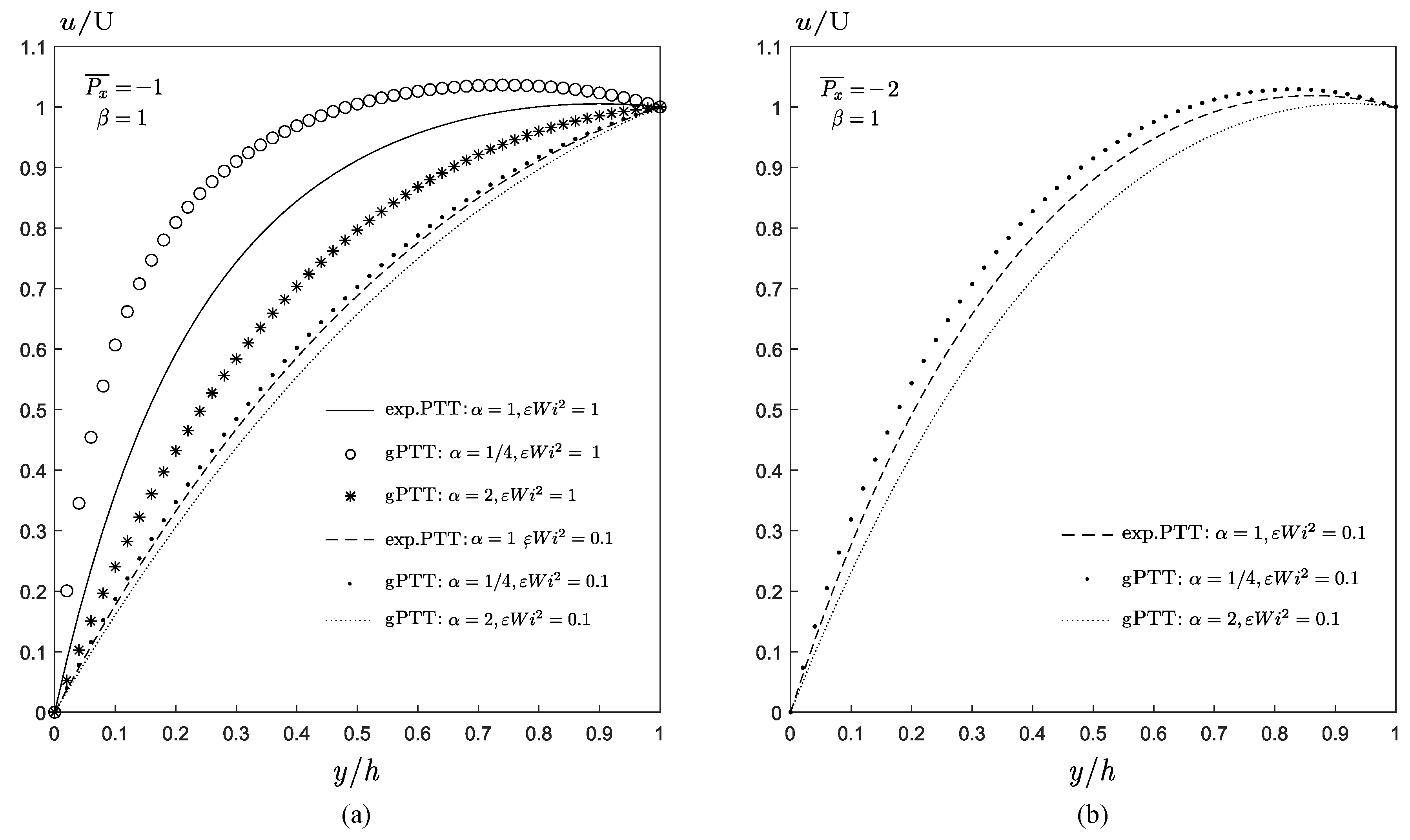
Combining Equations (31) and (32) leads to the following dimensionless velocity profile:

$$\overline{u}\left(\overline{y}\right)=\frac{\Gamma \left(\beta \right)}{\overline{P_x}}\sum _{k=0}^{\infty }\left({\left(2\epsilon {Wi}^2\right)}^k\frac{1}{\Gamma (\alpha k+\beta )}\frac{{\left(\overline{P_x}\overline{y}+\overline{c_1}\right)}^{2k+2}-{\overline{c_1}}^{2k+2}}{2k+2}\right)$$

(33)

with $\overline{y}=\frac{y}{h}$, $\overline{u}\left(y\right)=\frac{u\left(\overline{y}\right)}{\mathrm{U}}$, $\overline{c_1}=\frac{c_{1}h}{{\eta }_p\mathrm{U}}$, $\overline{P_x}=\frac{P_x{h}^2}{{\eta }_p\mathrm{U}}$ and $Wi=\frac{\lambda \mathrm{U}}{h}$ the Weissenberg number.

Remark 1.

Note that, if $c_1=-P_x\frac{h}{2}$, Equation (31) becomes,

$$u\left(y\right)=\mathrm{U}-\frac{\Gamma \left(\beta \right)}{{\eta }_p{P}_x}\sum _{k=0}^{\infty }\left({\left(\frac{2\epsilon {\lambda }^2}{{\eta }_p^2}\right)}^k\frac{1}{\Gamma (\alpha k+\beta )}\frac{{\left(P_x\frac{h}{2}\right)}^{2k+2}-{\left(P_x\left(y-\frac{h}{2}\right)\right)}^{2k+2}}{2k+2}\right),$$

(34)

and Equation (32) leads to $u\left(h\right)=0$, corresponding to Poiseuille flow with no slip boundary conditions.

The velocity profile can be written in dimensionless form as:

$$\overline{u}\left(\overline{y}\right)=\frac{\Gamma \left(\beta \right)}{\overline{P_x}}\sum _{k=0}^{\infty }\left({\left(2\epsilon {Wi}^2\right)}^k\frac{1}{\Gamma (\alpha k+\beta )}\frac{{\left(\overline{P_x}\left(\overline{y}-\frac{1}{2}\right)\right)}^{2k+2}-{\left(\frac{\overline{P_x}}{2}\right)}^{2k+2}}{2k+2}\right).$$

(35)

When we consider $\alpha =\beta =1$, this equation reduces to the one presented by Oliveira and Pinho [8] for the planar channel flow of an exponential PTT fluid:

$$\overline{u}\left(\overline{y}\right)=\frac{1}{4\epsilon {Wi}^2\overline{P_x}}\left(exp\left(2\epsilon {Wi}^2{\overline{P_x}}^2{\left(\overline{y}-\frac{1}{2}\right)}^2\right)-exp\left(\frac{2\epsilon {Wi}^2{\overline{P_x}}^2}{4}\right)\right).$$

(36)

Figure 4 shows a comparison between the gPTT model and exponential PTT (Equations (35) and (36)) for different values of $\epsilon W{i}^2$. As expected, the results are identical, confirming the solution limit for $\alpha =\beta =1$ on the Mittag–Leffler function.

3. Analytical Solution for the gPTT Model in Pure Couette flow.

For the pure Couette flow, $P_x=0$, therefore Equation (24) becomes,

$${\tau }_{xy}=c_1.$$

(37)

The shear rate is then given by Equation (38),

$$\dot{\gamma }\left(y\right)=\Gamma \left(\beta \right)E_{\alpha ,\beta }\left(\frac{2\epsilon {\lambda }^2}{{\eta }_p^2}{c_1}^2\right)\frac{c_1}{{\eta }_p}.$$

(38)

Integrating Equation (38) and taking into account Equation (29), the velocity field for the pure Couette flow is obtained,

$$u\left(y\right)=\frac{\Gamma \left(\beta \right)}{{\eta }_p}\sum _{k=0}^{\infty }\left({\left(\frac{2\epsilon {\lambda }^2}{{\eta }_p^2}\right)}^k\frac{c_1^{2k+1}}{\Gamma (\alpha k+\beta )}y\right).$$

(39)

Making use of the boundary condition given in Equation (30), we obtain the following nonlinear equation on $c_1$, which must be solved numerically,

$$\frac{\mathrm{U}}{h}=\frac{\Gamma \left(\beta \right)}{{\eta }_p}\sum _{k=0}^{\infty }\left({\left(\frac{2\epsilon {\lambda }^2}{{\eta }_p^2}\right)}^k\frac{c_1^{2k+1}}{\Gamma (\alpha k+\beta )}\right).$$

(40)

Equations (39) and (40) can be written in dimensionless form as:

$$\overline{u}\left(\overline{y}\right)=\Gamma \left(\beta \right)\overline{c_1}\overline{y}\sum _{k=0}^{\infty }\left({\left(2\epsilon W{i}^2{\overline{c_1}}^2\right)}^k\frac{1}{\Gamma (\alpha k+\beta )}\right)$$

(41)

and

$$1=\Gamma \left(\beta \right)\overline{c_1}\sum _{k=0}^{\infty }\left({\left(2\epsilon W{i}^2{\overline{c_1}}^2\right)}^k\frac{1}{\Gamma (\alpha k+\beta )}\right),$$

(42)

respectively.

4. Discussion of Results

In the previous section, semi-analytical equations were derived for the gPTT model in Poiseuille–Couette flow. In this section, we investigate the influence of the Mittag–Leffler function parameters $\alpha$ and $\beta$ on the velocity profile of the Poiseuille–Couette flow. We consider different $\epsilon W{i}^2$ values, and also different values of $\alpha$ and $\beta$, and we compare the results with the ones obtained for the exponential PTT model. Figure 5 shows the velocity profiles obtained for the Poiseuille–Couette flow considering two different $\epsilon W{i}^2$ values and different values of $\alpha$ ($\beta =1$).

Figure 6 shows the velocity profiles obtained for the Poiseuille–Couette flow considering two different $\epsilon {Wi}^2$ and different values of $\beta$ ($\alpha =1$).

We observe in Figure 5a that for $\alpha >1$ the flow rate decreases while for $\alpha <1$ it increases. As expected, for a constant pressure drop, the flow rate increases with $\epsilon W{i}^2$. In Figure 5b, we can observe that with the increase of the absolute value of the pressure drop, the velocity profile becomes more sensitive to small changes in $\alpha$.

For the case of constant $\alpha =1$ and varying $\beta$ (Figure 6), the trends are similar to the ones obtained in Figure 5 (varying $\alpha$), but now the velocity profile is less sensitive to large vales of $\beta$ (with $\beta >1$). In Figure 6b, we observe that the combined effects of pressure drop and large values of $\epsilon W{i}^2$ lead to a substantial increase of the flow rate for $\beta <1$.

5. Conclusions

In this work, we develop new analytical solutions for the Poiseuille–Couette flow of a viscoelastic fluid modelled by the generalised PTT model. We study the influence of the model’s new parameters on the velocity profile and we discuss the role of the new function of the stress tensor on weak flows. The new model allows a broader description of flow behavior, and therefore it should be considered in the modelling of complex viscoelastic flows. The analytical solutions developed in this work are helpful for validating CFD codes, and also allow a further understanding of the model behavior in weak flows.

References

1. Bird, R.B.; Armstrong, R.C.; Hassager, O. Dynamics of Polymeric Liquids. Volume 1: Fluid Mechanics; John Wiley & Sons: Hoboken, NJ, USA, 1987. [Google Scholar]
2. Ferrás, L.L.; Morgado, M.L.; Rebelo, M.; McKinley Gareth, H.; Afonso, A.M. A Generalised Phan-Thien-Tanner Model. J. Non-Newton. Fluid Mech. 2019, 269, 88–99. [Google Scholar] [CrossRef]
3. Phan-Thien, N.; Tanner, R. A new constitutive equation derived from network theory. J. Non-Newton. Fluid Mech. 1977, 2, 353–365. [Google Scholar] [CrossRef]
4. Phan-Thien, N. A Nonlinear Network Viscoelastic Model. J. Rheol. 1978, 22, 259–283. [Google Scholar] [CrossRef]
5. Podlubny, I. Fractional Differential Equations: An Introduction to Fractional Derivatives, Fractional Differential Equations, to Methods of Their Solution and Some of Their Applications; Elsevier: Amsterdam, The Netherlands, 1998; Volume 198. [Google Scholar]
6. Ferrás, L.L.; Afonso, A.M.; Alves, M.A.; Nóbrega, J.M.; Pinho, F.T. Annular flow of viscoelastic fluids: Analytical and numerical solutions. J. Non-Newton. Fluid Mech. 2014, 212, 80–91. [Google Scholar] [CrossRef] [Green Version]
7. Laun, H.M. Description of the non-linear shear behaviour of a low density polyethylene melt. Rheol. Acta 1978, 17, 1–15. [Google Scholar] [CrossRef]
8. Oliveira, P.J.; Pinho, F.T. Analytical solution for fully developed channel and pipe flow of Phan-Thien-Tanner fluids. J. Fluid Mech. 1999, 387, 271–280. [Google Scholar] [CrossRef]
Figure 1. Dimensionless material properties in steady-state Couette flow using the three versions of the sPTT and for the gPTT model: (a) β = 1 ; and (b) α = 1 .
Fluids 04 00129 g001
Figure 2. Fitting of the shear viscosity and the first normal stress difference coefficient to rheological data from Laun [7]. The generalised PTT model only considers the one-parameter Mittag–Leffler function, E α . By adding only one parameter, we obtain a fitting error (Equation (17)) of 29 . 7 and 6 for the exponential and gPTT models, respectively. The symbols represent the experimental data from Laun [7] for a low density polyethylene melt.
Fluids 04 00129 g002
Figure 3. Geometry of: (a) the pure Couette flow; and (b) the Couette flow with an imposed pressure gradient (Poiseuille–Couette flow).
Fluids 04 00129 g003
Figure 4. Comparison between the gPTT model and exponential PTT considering a Poiseuille flow with different values of ε W i 2 and different values of imposed P x ¯ .
Fluids 04 00129 g004
Figure 5. Velocity profiles obtained for the Poiseuille–Couette flow considering different values of ε W i 2 and different values of α ( β = 1 ): (a) P x ¯ = - 1 ; and (b) P x ¯ = - 2 .
Fluids 04 00129 g005
Figure 6. Velocity profiles obtained for the Poiseuille–Couette flow considering different values of ε W i 2 and different values of β ( α = 1 ): (a) P x ¯ = - 1 ; and (b) P x ¯ = - 2 .
Fluids 04 00129 g006