A New Exact Solution for the Flow of a Fluid through Porous Media for a Variety of Boundary Conditions

 ,
,  and
and 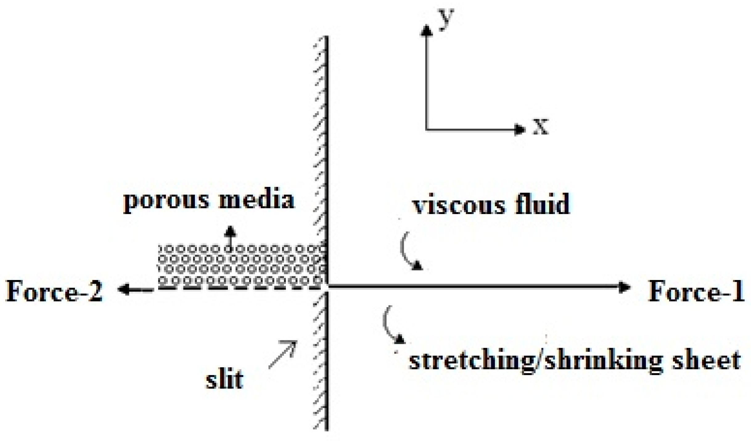
Abstract
1. Introduction
2. Theoretical Model
3. The Analytical Solution
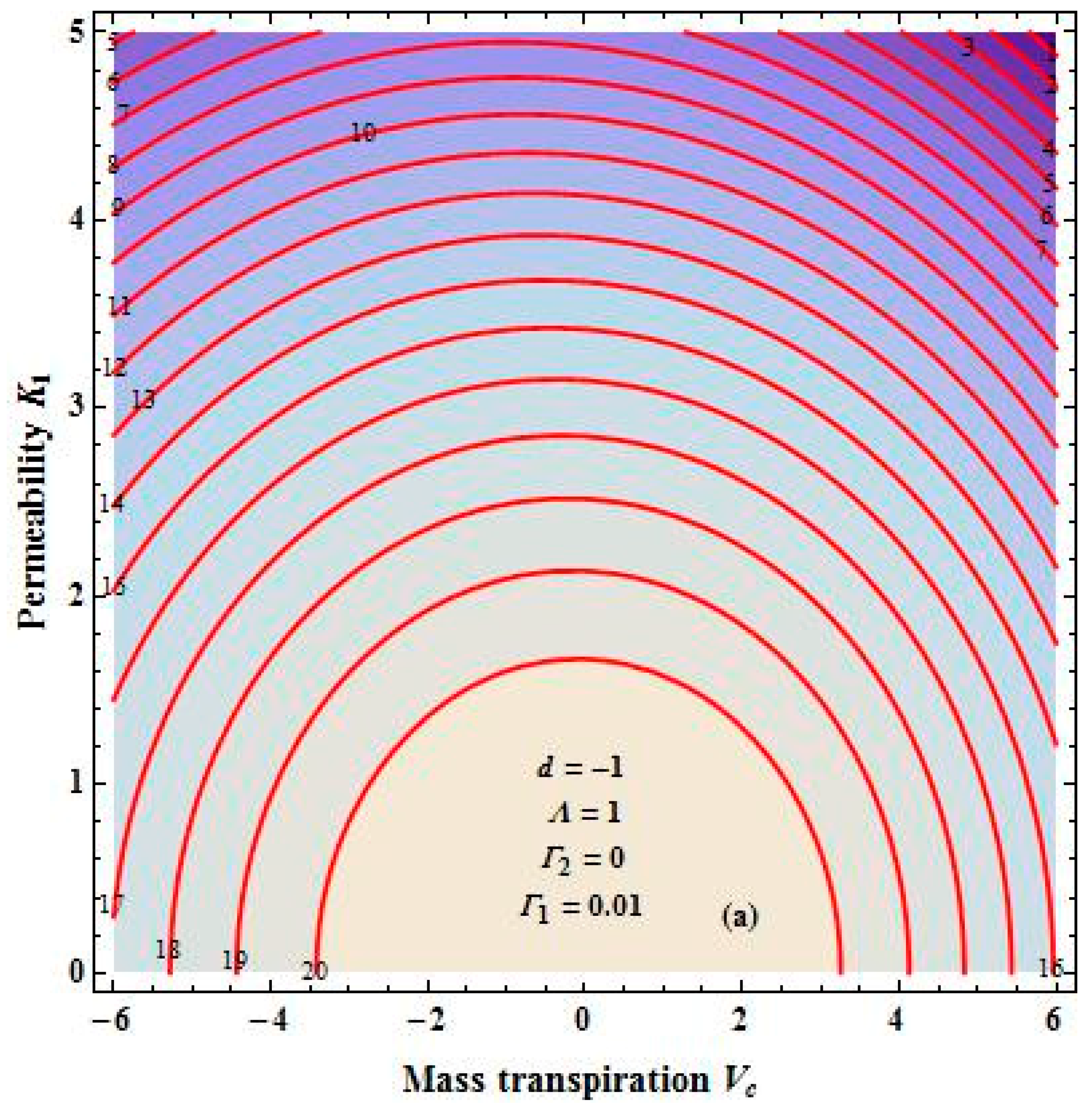
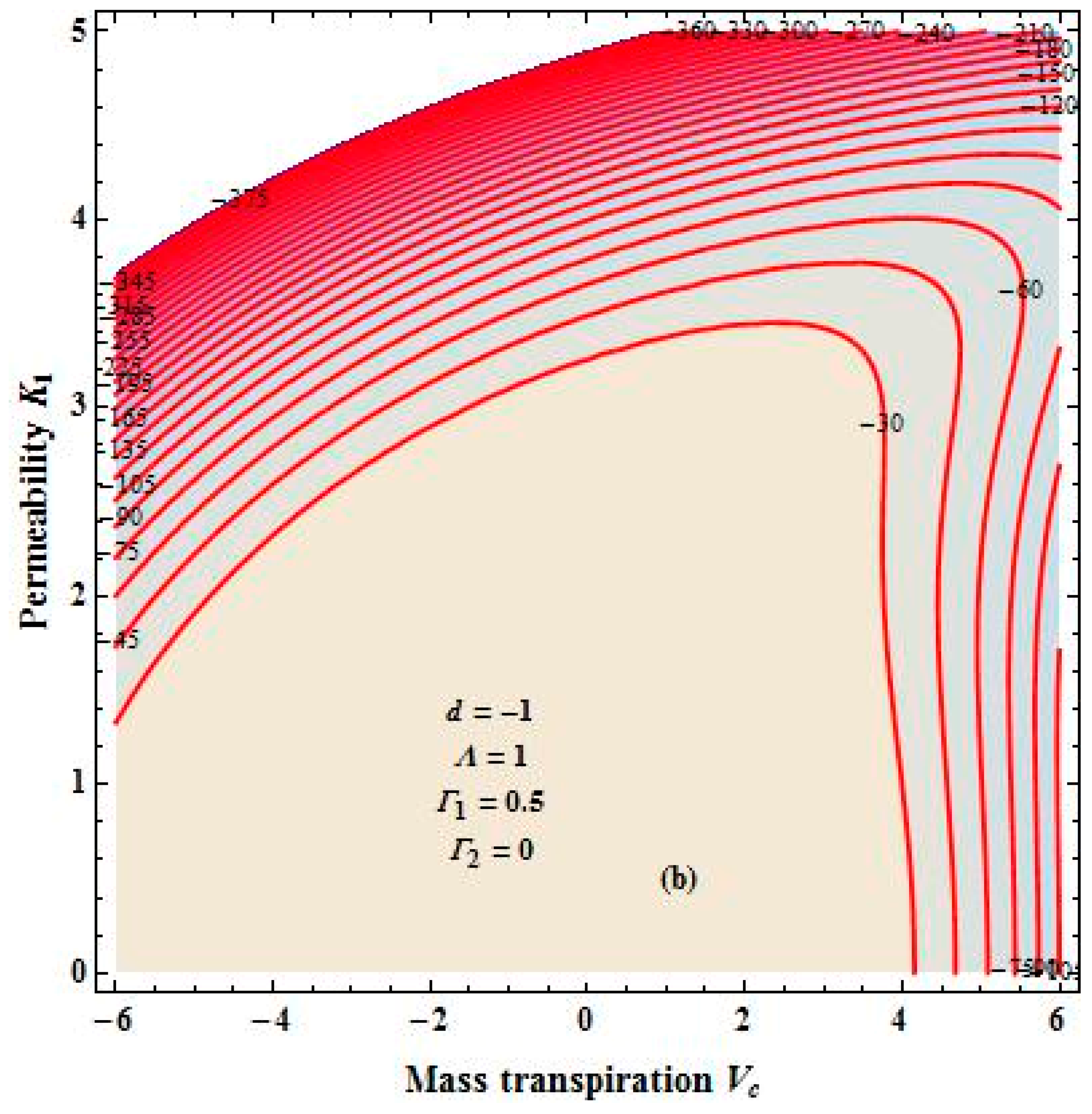
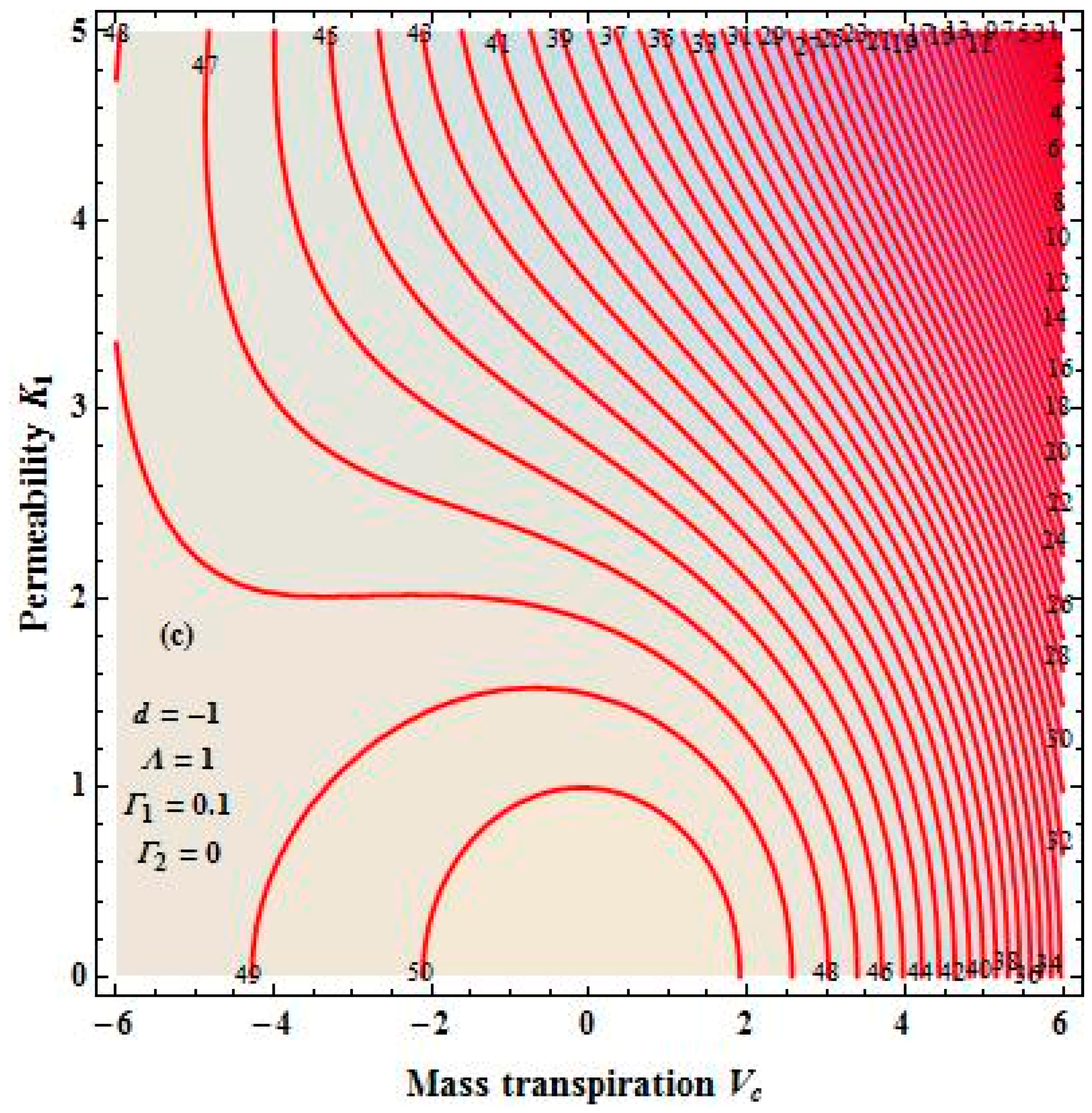
4. Results and Discussion
5. Concluding Remarks
Author Contributions
Funding
Acknowledgments
Conflicts of Interest
References
- Fisher, B.G. Extrusion of Plastics, 3rd ed.; Newnes-Butterworld: London, UK, 1976. [Google Scholar]
- Brinkman, H.C. On the permeability of the media consisting of closely packed porousparticles. Appl. Sci. Res. 1947, 1, 81–86. [Google Scholar] [CrossRef]
- Darcy, H. Les Fontaines Publiques De La Ville De Dijon; Victor Dalmont: Paris, France, 1856. [Google Scholar]
- Forchheimer, P. Wasserbewegung Durch Boden; Zeitschrift des Vereines Deutscher In-Geneieure: Düsseldorf, Germany, 1901; Volume 45, pp. 1782–1788. [Google Scholar]
- Biot, M.A. Mechanics of Deformation and Acoustic Propagation in Porous Media. J. Appl. Phys. 1962, 33, 1482–1498. [Google Scholar] [CrossRef]
- Truesdell, C. Sulla basi della thermomechanical. Rend. Lincei 1957, 22a, 158–166. [Google Scholar]
- Truesdell, C. Sulla basi della thermomechanical. Rend. Lincei 1957, 22b, 33–38. [Google Scholar]
- Chakrabarti, A.; Gupta, A.S. Hydromagnetic flow and heat transfer over a stretching sheet. Q. Appl. Math. 1979, 37, 73–78. [Google Scholar] [CrossRef]
- Gupta, P.S.; Gupta, A.S. Heat and mass transfer on a stretching sheet with suction or blowing. Can. J. Chem. Eng. 1977, 55, 744–746. [Google Scholar] [CrossRef]
- Fang, T. Boundary layer flow over a shrinking sheet with power-law velocity. Int. J. Heat Mass Transf. 2008, 51, 5838–5843. [Google Scholar] [CrossRef]
- Milavcic, M.; Wang, C.Y. Viscous flow due to a shrinking sheet. Q. Appl. Math. 2006, 64, 283–290. [Google Scholar] [CrossRef]
- Nakayama, A. PC-Aided Numerical Heat Transfer and Convective Flow; CRC Press: Boca Raton, FL, USA, 1995. [Google Scholar]
- Sakiadis, B.C. Boundary-layer behavior on continuous solid surface. AIChE J. 1961, 7, 26–28. [Google Scholar] [CrossRef]
- Sakiadis, B.C. Boundary-layer behavior on continuous solid surfaces. II. The boundary layer on a continuous flat surface. AIChE J. 1961, 7, 221–225. [Google Scholar] [CrossRef]
- Rajagopal, K.R.; Tao, L. Mechanics of Mixtures; World Scientific: Singapore, 1995. [Google Scholar]
- Givler, R.C.; Altobelli, S.A. A Determination of the Effective Viscosity for the Brinkman-Forchheimer Flow Model. J. Fluid Mech. 1994, 258, 355–370. [Google Scholar] [CrossRef]
- Shao, Q.; Fahs, M.; Hoteit, H.; Carrera, J.; Ackerer, P.; Younes, A. A 3D semi-analytical solution for density-driven flow in porous media. Water Res. Res. 2018, 54, 10094–10116. [Google Scholar] [CrossRef]
- Lesinigo, M.; D’Angelo, C.; Quarteroni, A. A multiscale Darcy-Brinkman model for fluid flow in fractured porous media. Numer. Math. 2011, 117, 717–752. [Google Scholar] [CrossRef]
- Murali, K.; Naidu, V.K.; Venkatesh, B. Solution of Darcy-Brinkman-Forchheimer Equation for Irregular Flow Channel by Finite Elements Approach. J. Phys. Conf. Ser. 2019, 1172, 012033. [Google Scholar] [CrossRef]
- Kumaran, V.; Tamizharasi, R. Pressure in MHD/Brinkman flow past a stretching sheet. Commun. Nonlinear Sci. Numer. Simul. 2011, 16, 4671–4681. [Google Scholar]
- Nield, D.A.; Bejan, A. Convection in Porous Media; Springer Verlag Inc.: New York, NY, USA, 1998. [Google Scholar]
- Nield, D.A.; Kuznetsov, A.V. Forced convection in porous media: Transverse heterogeneity effects and thermal development. In Handbook of Porous Media, 2nd ed.; Vafai, K., Ed.; Taylor and Francis: New York, NY, USA, 2005; pp. 143–193. [Google Scholar]
- Nield, D.A. The modeling of viscous dissipation in a saturated porous medium. J. Heat Transf. 2007, 129, 1459–1463. [Google Scholar] [CrossRef]
- Nield, D.A.; Bejan, A. Convection in Porous Media, 4th ed.; Springer: New York, NY, USA, 2013. [Google Scholar]
- Pantokratoras, A. Flow adjacent to a stretching permeable sheet in a Darcy-Brinkman porous medium. Transp. Porous Med. 2009, 80, 223–227. [Google Scholar] [CrossRef]
- Pop, I.; Ingham, D.B. Flow past a sphere embedded in a porous medium based on the Brinkman model. Int. Commun. Heat Mass Transf. 1996, 23, 865–874. [Google Scholar] [CrossRef]
- Pop, I.; Na, T.Y. A note on MHD flow over a stretching permeable surface. Mech. Res. Commun. 1998, 25, 263–269. [Google Scholar] [CrossRef]
- Pop, I.; Cheng, P. Flow past a circular cylinder embedded in a porous medium based on the Brinkman model. Int. J. Eng. Sci. 1992, 30, 257–262. [Google Scholar] [CrossRef]
- Wang, C.Y. Darcy-Brinkman Flow with Solid Inclusions. Chem. Eng. Commun. 2010, 197, 261–274. [Google Scholar] [CrossRef]
- Srinivasan, S.; Rajagopal, K.R. A thermodynamic basis for the derivation of the Darcy, Forchheimer and Brinkman models for flows through porous media and their generalizations. Int. J. Non-Linear Mech. 2014, 58, 162–166. [Google Scholar] [CrossRef]
- Ingham, D.B.; Pop, I. Transport in Porous Media; Pergamon: Oxford, UK, 2002. [Google Scholar]
- Magyari, E.; Keller, B. Exact solutions for self-similar boundary-layer flows induced by permeable stretching surfaces. Eur. J. Mech. B 2000, 19, 109–122. [Google Scholar] [CrossRef]
- Mastroberardino, A.; Mahabaleshwar, U.S. Mixed convection in viscoelastic flow due to a stretching sheet in a porous medium. J. Porous Media 2013, 16, 483–500. [Google Scholar] [CrossRef]
- Siddheshwar, P.G.; Mahabaleshwar, U.S. Effects of radiation and heat source on MHD flow of a viscoelastic liquid and heat transfer over a stretching sheet. Int. J. Non-Linear Mech. 2005, 40, 807–820. [Google Scholar] [CrossRef]
- Siddheshwar, P.G.; Chan, A.; Mahabaleshwar, U.S. Suction-induced magnetohydrodynamics of a viscoelastic fluid over a stretching surface within a porous medium. IMA J. Appl. Math. 2014, 79, 445–458. [Google Scholar] [CrossRef]
- Tamayol, A.; Hooman, K.; Bahrami, M. Thermal analysis of flow in a porous medium over a permeable stretching wall. Transp. Porous Media 2010, 85, 661–676. [Google Scholar] [CrossRef]
- Shao, Q.; Fahs, M.; Younes, A.; Makradi, A. A High Accurate Solution for Darcy-Brinkman Double-Diffusive Convection in Saturated Porous Media. J. Numer. Heat Transf. Part B Fundam. 2015, 69, 26–47. [Google Scholar] [CrossRef]
- Navier, C.L.M.H. Mémoire sur les lois du mouvement des fluids. Mém. Acad. R. Sci. Inst. Fr. 1827, 6, 389–440. [Google Scholar]
- Brinkman, H.C. A calculation of the viscous force exerted by a flowing fluid on a dense swarm of particles. Appl. Sci. Res. 1949, 1, 27–34. [Google Scholar] [CrossRef]
- Mahabaleshwar, U.S.; Nagaraju, K.R.; Kumar, P.N.V.; Baleanu, D.; Lorenzini, G. An exact analytical solution of the unsteady magnetohydrodynamics nonlinear dynamics of laminar boundary layer due to an impulsively linear stretching sheet. Contin. Mech. Thermodyn. 2017, 29, 559–567. [Google Scholar] [CrossRef]
- Rajagopal, K.R. On a hierarchy of approximate models for flows of incompressible fluids through porous solids. Math. Model. Methods Appl. Sci. 2007, 17, 215–252. [Google Scholar] [CrossRef]
- Vafai, K.; Tien, C.L. Boundary and inertia effects on flow and heat transfer in porous media. Int. J. Heat Mass Transf. 1981, 24, 195–203. [Google Scholar] [CrossRef]
- Fang, T.; Aziz, A. Viscous flow with second-order slip velocity over a stretching sheet. Zeitschrift Für Naturforschung A 2010, 65, 1087–1092. [Google Scholar] [CrossRef]
- Lin, W. Mass transfer induced slip effect on viscous gas flows above a shrinking/stretching sheet. Int. J. Heat Mass Transf. 2016, 93, 17–22. [Google Scholar]
- Andersson, H.I. Slip flow past a stretching surface. Acta Mech. 2002, 158, 121–125. [Google Scholar] [CrossRef]
- Crane, L.J. Flow past a stretching plate. Z. Angew. Math. Phys. 1970, 21, 645–647. [Google Scholar] [CrossRef]
- Pavlov, K.B. Magnetohydrodynamic flow of an incompressible viscous liquid caused by deformation of plane surface. Magn. Gidrodin. 1974, 4, 146–147. [Google Scholar]
- Wang, C.Y. Flow due to a stretching boundary with partial slip—An exact solution of the Navier-Stokes equations. Chem. Eng. Sci. 2002, 57, 3745–3747. [Google Scholar] [CrossRef]
- Abramowitz, M.; Stegun, I.A. Handbook of Mathematical Functions with Formulas, Graphs, and Mathematical Tables, 9th ed.; Dover: New York, NY, USA, 1972; pp. 17–18. [Google Scholar]
- Birkhoff, G.; MacLane, S. A Survey of Modern Algebra; Macmillan: New York, NY, USA, 1996; pp. 107–108. [Google Scholar]
- Fang, T.-G.; Zhang, J.; Yao, S.-S. Slip Magnetohydrodynamic Viscous Flow over a Permeable Shrinking Sheet. Chin. Phys. Lett. 2010, 27, 124702. [Google Scholar] [CrossRef]
- Fang, T.; Yao, S.; Zhang, J.; Aziz, A. Viscous flow over a shrinking sheet with a second order slip flow model. Commun. Nonlinear Sci. Numer. Simul. 2010, 15, 1831–1842. [Google Scholar] [CrossRef]


© 2019 by the authors. Licensee MDPI, Basel, Switzerland. This article is an open access article distributed under the terms and conditions of the Creative Commons Attribution (CC BY) license (http://creativecommons.org/licenses/by/4.0/).
Share and Cite
Mahabaleshwar, U.S.; Vinay Kumar, P.N.; Nagaraju, K.R.; Bognár, G.; Nayakar, S.N.R. A New Exact Solution for the Flow of a Fluid through Porous Media for a Variety of Boundary Conditions. Fluids 2019, 4, 125. https://doi.org/10.3390/fluids4030125
Mahabaleshwar US, Vinay Kumar PN, Nagaraju KR, Bognár G, Nayakar SNR. A New Exact Solution for the Flow of a Fluid through Porous Media for a Variety of Boundary Conditions. Fluids. 2019; 4(3):125. https://doi.org/10.3390/fluids4030125
Chicago/Turabian StyleMahabaleshwar, U. S., P. N. Vinay Kumar, K. R. Nagaraju, Gabriella Bognár, and S. N. Ravichandra Nayakar. 2019. "A New Exact Solution for the Flow of a Fluid through Porous Media for a Variety of Boundary Conditions" Fluids 4, no. 3: 125. https://doi.org/10.3390/fluids4030125
APA StyleMahabaleshwar, U. S., Vinay Kumar, P. N., Nagaraju, K. R., Bognár, G., & Nayakar, S. N. R. (2019). A New Exact Solution for the Flow of a Fluid through Porous Media for a Variety of Boundary Conditions. Fluids, 4(3), 125. https://doi.org/10.3390/fluids4030125