A Potential Field Description for Gravity-Driven Film Flow over Piece-Wise Planar Topography

Abstract

Models based on a potential field description and corresponding first integral formulation, embodying a reduction of the associated dynamic boundary condition at a free surface to one of a standard Dirichlet-Neumann type, are used to explore the problem of continuous gravity-driven film flow down an inclined piece-wise planar substrate in the absence of inertia. Numerical solutions of the first integral equations are compared with analytical ones from a linearised form of a reduced equation set resulting from application of the long-wave approximation. The results obtained are shown to: (i) be in very close agreement with existing, comparable experimental data and complementary numerical predictions for isolated step-like topography available in the open literature; (ii) exhibit the same qualitative behaviour for a range of Capillary numbers and step heights/depths, becoming quantitively similar when both are small. A novel outcome of the formulation adopted is identification of an analytic criteria enabling a simple classification procedure for specifying the characteristic nature of the free surface disturbance formed; leading subsequently to the generation of a related, practically relevant, characteristic parameter map in terms of the substrate inclination angle and the Capillary number of the associated flow.

1. Introduction

Film flow on rigid substrates that are either locally non-planar, due to the presence of isolated topographical features, or exhibit a periodically repeating pattern of the same, has been the topic of considerable research interest over the past four decades or so, motivated by such occurrences in numerous industrially relevant fields. These include, for example, the manufacture of micro-scale sensors and devices [1], thin-film transistors [2], organic light-emitting diode (OLED) displays [3], printed circuits [4], and the deposition of functional coatings using slot-die and slide/cascade arrangements [5]. Cumulatively, this has led to a better understanding of important and interrelated phenomena, using gravity-driven film flow in particular as a an investigative platform: ranging from the unwanted free surface disturbances generated by randomly occurring or prescribed micro-scale substrate irregularities, which in turn can become a feature of the final coated product once drying has taken place [6], to the susceptibility of such flows to loss of stability and whether the presence of topography can lead to a delayed onset compared to film flow on completely planar substrate.

Significant contributions to the field experimentally are the early investigations of [7,8,9] and more recently those of [10,11,12] covering both steady films and routes to instability. Much of the associated theoretical and predictive contributions have used models assuming the existence of a steady flow employing the long-wave approximation [13], leading to a lubrication or integral boundary layer approximation, with the corresponding equation sets solved numerically [14]. Of note is the combined work of Kalliadasis et al. [15], Mazouchi and Homsy [16] and the comprehensive numerical solutions of Gaskell et al. [17], the results of which being in very good agreement with the experimentally captured free surface data of Decré and Baret [10]. In addition, [17] provide a very detailed quantitative parameter study and error analysis of the effect of Reynolds number and flow rate with regard to topography height/depth. The same flow problems were considered a decade later by Veremieiev et al. [18] using a depth averaged form of the NS equations, confirming their findings. Note also that Hayes et al. [19] used a lubrication approximation to model the case of thin film flow over a small particle arrested at a wall, represented as a Dirac function, far exceeding the strict requirements of the underlying assumptions; nevertheless, their results were similarly shown to be realistic when compared against experiment [10].

Few related numerical solutions, of a finite or boundary element type, have appeared focusing in particular on the behaviour of the accompanying 2D flow structure within the film [20] and in the case of 3D flow [21,22,23]; other, related investigations, have used a volume of fluid approach to explore pattern formation and mixing in film flow [24], surface wetting [25], together with the evolution of a single rivulet and its breakup [26,27].

Complementary stability analyses have become increasingly available [28,29,30], revealing interesting features concerning the effect of periodically repeating topography on the stability of films, showing the critical Reynolds number signalling the onset of instability, compared to the corresponding value predicted for film flow on totally planar substrate, is increased. Resulting even in the re-establishment of islands of stability as the Reynolds number is increased further still—in this respect the reader is directed to the following recent contributions [31,32,33,34,35]

In connection with the issue of minimising/controlling the free surface disturbance associated with film flow over topography, others have considered the inverse problem of substrate design based on information concerning the free surface, [36,37,38], non-Newtonian effects [39] and the the influence of electric fields [40,41].

The remainder of the manuscript proceeds as follows. The modelling approaches adopted and the corresponding equation sets are developed in Section 2, with solutions obtained in one of two ways, as found in Section 3. Numerically in the case of the first integral equations; analytically by invoking the long-wave approximation which for zero Reynolds number reduces the entire problem to a set of two nonlinear ODEs that are shown to recover the well known degenerate Nusselt solution for film flow on completely planar substrate. Linearisation of these equations to first order, in terms of a sufficiently small value of the ratio of topography height to asymptotic film thickness, as performed in Section 4, leads to analytical solutions for flow over piece-wise features which: (i) compare well to their numerical counterparts and ones in the open literature; (ii) facilitate the construction of a practically useful characteristic parameter map describing the expected nature of the accompanying free surface disturbance. Conclusions are drawn and potential future applications of the method discussed in Section 5.

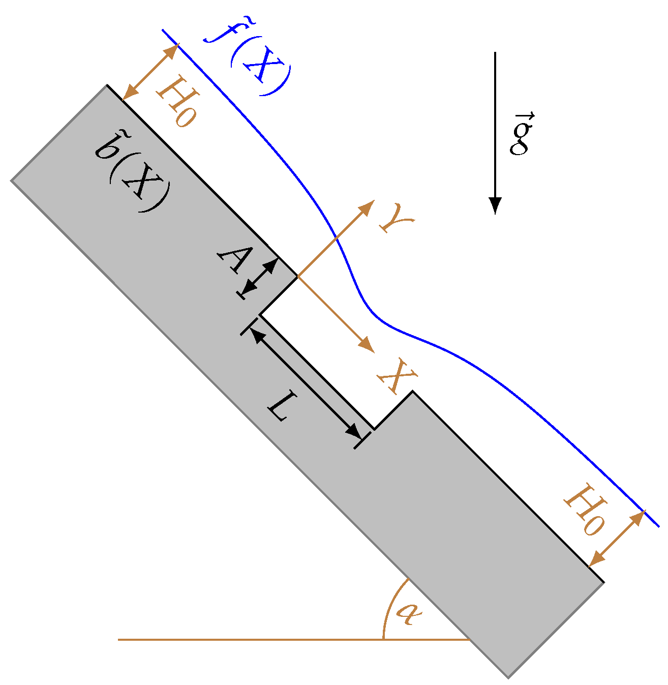
2. Problem Specification and Model Formulations

A schematic of the problem of interest is provided in Figure 1; it shows the associated coordinate system and geometry, for the case of film flow, asymptotic thickness $H_0$, down a piece-wise planar substrate containing, for illustration purposes only, a sharp-sided trench topography of depth A and length L. For sufficiently large L the problem reduces to one of flow over a step-down followed by a step-up [16,17]. This general problem definition similarly applies to the situation of flow over an equal but opposite peak topography and to smoothly varying topographical features.

2.1. Standard Formulation

The liquid film is assumed to be Newtonian and incompressible with the flow governed by the corresponding steady-state NS and Continuity equations:

$$\begin{array}{ccc}\hfill \varrho \left[U\frac{\partial U}{\partial X}+V\frac{\partial U}{\partial Y}\right]& =& -\frac{\partial P}{\partial X}+\eta \left[\frac{{\partial }^{2}U}{\partial X^2}+\frac{{\partial }^{2}U}{\partial Y^2}\right]+\varrho gsin\left(\alpha \right),\hfill \end{array}$$

(1)

$$\begin{array}{ccc}\hfill \varrho \left[U\frac{\partial V}{\partial X}+V\frac{\partial V}{\partial Y}\right]& =& -\frac{\partial P}{\partial Y}+\eta \left[\frac{{\partial }^{2}V}{\partial X^2}+\frac{{\partial }^{2}V}{\partial Y^2}\right]-\varrho gcos\left(\alpha \right),\hfill \end{array}$$

(2)

$$\begin{array}{cc}\hfill \frac{\partial U}{\partial X}+\frac{\partial V}{\partial Y}=& 0,\hfill \end{array}$$

(3)

where U, V and $gcos\left(\alpha \right)$, $gsin\left(\alpha \right)$ denote the the velocity and body force components parallel and perpendicular to the substrate, respectively; P is the pressure, $\varrho$ the density and $\eta$ the dynamic viscosity.

The problem constitutes a simply connected domain containing a free surface given by $\overrightarrow{X}=\overrightarrow{X}\left(S\right)$; that is, the free surface is assumed to be parametrised with respect to its arclength S. In two dimensions its shape is determined by one kinematic ($\overrightarrow{U}·\overrightarrow{n}=0$) and two dynamic boundary conditions:

$${\left[(P_0-P)\overrightarrow{n}+\eta \left(\nabla \otimes \overrightarrow{U}+{\left[\nabla \otimes \overrightarrow{U}\right]}^t\right)\overrightarrow{n}\right]}_{\overrightarrow{X}=\overrightarrow{X}\left(S\right)}=\sigma \frac{\mathrm{d}\overrightarrow{t}}{\mathrm{d}S},$$

(4)

with normal vector $\overrightarrow{n}$, tangential vector $\overrightarrow{t}$ and $\sigma$ denoting the surface tension. At the piece-wise planar substrate, whose shape is characterised by $Y=\tilde{b}\left(X\right)$, the velocity field must fulfil the no-slip/no-penetration conditions $U=0$, $V=0$; while, sufficiently far away from the topographical feature of interest, both upstream and downstream, the Nusselt velocity profile for flow over a planar surface is assumed.

While the above formulation represents the usual starting point from which to theoretically investigate the flow of interest, as discussed in the Introduction, the thrust of the present contribution is based entirely on a related approach that employs a potential field description leading to a first integral formulation.

2.2. First Integral Formulation

In recent years, different first integral forms of the 2D-NS equations have appeared [42,43,44]; the present work employs the real-valued form given in Marner et al. [45]:

$$\begin{array}{c}\hfill \varrho \left(U^2-V^2\right)+2\left\{{\partial }_X^2-{\partial }_Y^2\right\}\mathsf{\Phi }-4\eta {\partial }_X{\partial }_Y\mathsf{\Psi }=0,\end{array}$$

(5)

$$\begin{array}{c}\hfill 2\varrho UV+4{\partial }_X{\partial }_Y\mathsf{\Phi }+2\eta \left\{{\partial }_X^2-{\partial }_Y^2\right\}\mathsf{\Psi }=0;\end{array}$$

(6)

where $\mathsf{\Phi }$ enters the problem via the relationship $P+\varrho {\overrightarrow{U}}^2/2+E=\Delta \mathsf{\Phi }$, and $E(X,Y)=\varrho g\left[sin\left(\alpha \right)X-cos\left(\alpha \right)Y\right]+E_0$ (with $E_0$ a constant that can be chosen arbitrarily) is the potential energy density of the conservative force. The Continuity equation is fulfilled identically by introducing a streamfunction $\mathsf{\Psi }$ in accordance with $U={\partial }_Y\mathsf{\Psi }$, $V=-{\partial }_X\mathsf{\Psi }$.

While the substrate boundary conditions are implemented in the usual way, there is an obvious benefit when it comes to applying those at the free surface via a first integral approach: the dynamic boundary conditions there can be reformulated more conveniently, Scholle et al. [44], by eliminating the pressure; leading to an integral formulation and revealing (4) to be a pure condition on the potential gradient, namely:

$$\underline{\epsilon }\nabla \mathsf{\Phi }\left(\overrightarrow{X}\left(S\right)\right)=\frac{\sigma }{2}\overrightarrow{t}\left(S\right)-\frac{1}{2}{\int }_{S_0}^{S}E\left(\overrightarrow{X}(\tilde{S})\right)\overrightarrow{n}(\tilde{S})\mathrm{d}\tilde{S},$$

(7)

where the entries in the tensor $\underline{\epsilon }$ are determined by the Levi-Civita symbol, i.e., ${\epsilon }_{12}=-{\epsilon }_{21}=1$ and ${\epsilon }_{11}={\epsilon }_{22}=0$, and the integral limit $S_0$ can be chosen arbitrarily. Furthermore, knowledge of the potential gradient at the free surface allows the derivation of Dirichlet and Neumann boundary conditions for the potential variable in the simply connected domain if $\mathsf{\Phi }$ is specified at a single point [45]. The kinematic boundary condition can be formulated as:

$$\mathsf{\Psi }(X,\tilde{f}(X))={\mathsf{\Psi }}_{\mathrm{s}}=\mathrm{const};$$

(8)

the unknown constant ${\mathsf{\Psi }}_{\mathrm{s}}$ indicating the flow rate and the free surface shape characterised in terms of the as yet unknown function $\tilde{f}\left(X\right)$ via $Y=\tilde{f}\left(X\right)$. After decomposition into component parts the first integral (7) of the dynamic boundary condition takes the form:

$$\begin{array}{cc}\hfill \frac{\partial \mathsf{\Phi }}{\partial X}+\frac{\sigma {\tilde{f}}^{\prime }\left(X\right)}{2\sqrt{1+{\tilde{f}}^{\prime }{\left(X\right)}^2}}-\frac{1}{2}\int E\left(X,\tilde{f}\left(X\right)\right)\mathrm{d}X& =0,\hfill \end{array}$$

(9)

$$\begin{array}{cc}\hfill \frac{\partial \mathsf{\Phi }}{\partial Y}-\frac{\sigma }{2\sqrt{1+{\tilde{f}}^{\prime }{\left(X\right)}^2}}-\frac{1}{2}\int E\left(X,\tilde{f}\left(X\right)\right){\tilde{f}}^{\prime }\left(X\right)\mathrm{d}X& =0,\hfill \end{array}$$

(10)

with E defined in terms of the integrals appearing in (9, 10) as:

$$\begin{array}{cc}\hfill \int E\left(X,\tilde{f}\left(X\right)\right)\mathrm{d}X& =\varrho g\left[cos\alpha \int \tilde{f}\left(X\right)\mathrm{d}X-\frac{1}{2}sin\alpha X^2\right]+E_{0}X+E_1,\hfill \end{array}$$

(11)

$$\begin{array}{cc}\hfill \int E\left(X,\tilde{f}\left(X\right)\right){\tilde{f}}^{\prime }\left(X\right)\mathrm{d}X& =\varrho g\left[\frac{1}{2}cos\alpha \tilde{f}{\left(X\right)}^2-sin\alpha \left(X\tilde{f}\left(X\right)-\int \tilde{f}\left(X\right)\mathrm{d}X\right)\right]+E_0\tilde{f}\left(X\right)+E_2,\hfill \end{array}$$

(12)

where the constants of integration $E_1,E_2$ can be chosen arbitrarily in the same way as $E_0$. For convenience $E_0=-\varrho gcos\alpha H_0$ is chosen; then $E_1=0$ and $E_2=\varrho gcos\alpha H_0^2/2$.

Subsequently, use is made of the following scalings. Taking $H_0$ as a characteristic length scale defines the corresponding non-dimensional quantities:

$$\begin{array}{c}\hfill (x,y)=\frac{(X,Y)}{H_0},a=\frac{A}{H_0},\ell =\frac{L}{H_0},h_0=1\end{array}$$

while a characteristic velocity scale based on a value equal to twice the corresponding free surface Nusselt velocity, denoted by $U_N=\varrho g{H}_0^{2}sin\left(\alpha \right)/\eta$, leads to the following scalings of the velocities $(U,V)$, potential field $\mathsf{\Phi }$, the streamfuction $\mathsf{\Psi }$ and the potential energy density $E(X,Y)$:

$$\begin{array}{c}\hfill (u,v)=\frac{(U,V)}{U_N},\varphi =\frac{\mathsf{\Phi }}{\eta U_N{H}_0},\psi =\frac{\mathsf{\Psi }}{U_N{H}_0},e(x,y)=\frac{E{H}_0}{\eta U_N}=cot\left(\alpha \right)y-x.\end{array}$$

The Reynolds and Capillary number is given by $\mathrm{Re}=\varrho U_N{H}_0/\eta$ and $\mathrm{Ca}=\eta U_N/\sigma$, respectively.

2.2.1. Lubrication Model

The first integral Equations (5) and (6) can be simplified based on a lubrication approximation, noting that the same applied to the NS equations, Stillwagon and Larson [8], leads to a single equation for the local film thickness; the velocity field to leading order being locally parabolic. The requirement underpinning its applicability in the case of topography exhibiting step-like changes is that the commensurate free surface disturbance is slowly varying which is indeed the case; film flow over step-like topographical features have been investigated successfully by many authors within a lubrication framework, as highlighted in the Introduction.

Neglecting ${\partial }_{X}V=-{\partial }_X^2\mathsf{\Psi }$ compared to ${\partial }_{Y}U={\partial }_Y^2\mathsf{\Psi }$ and omitting the inertial term, $2\varrho UV$, in Equation (6), results in the following simplified equation:

$${\partial }_Y\left[2{\partial }_X\mathsf{\Phi }-\eta {\partial }_Y\mathsf{\Psi }\right]=0,$$

which can be integrated with respect to Y to give:

$$2{\partial }_X\mathsf{\Phi }=\eta {\partial }_Y\mathsf{\Psi }+F_1\left(X\right),$$

(13)

the function $F_1\left(X\right)$ appearing as a consequence. By inserting (13) into (5) and neglecting, as above, the inertial term, $\varrho \left(U^2-V^2\right)$, leads to the following relationship

$${\partial }_Y\left[2{\partial }_Y\mathsf{\Phi }+3\eta {\partial }_X\mathsf{\Psi }\right]=F_1^{\prime }\left(X\right),$$

which when integrated with respect to Y, gives:

$$2{\partial }_Y\mathsf{\Phi }=-3\eta {\partial }_X\psi +F_1^{\prime }\left(X\right)Y+F_2\left(X\right),$$

(14)

with appearance of the function $F_2\left(X\right)$. Taking the derivative of (13) with respect to Y and that of (14) with respect to X, and combining the two, ${\partial }_Y$(13)$-{\partial }_X$(14), eliminates the potential $\mathsf{\Phi }$, leading to:

$$0=\eta \left[{\partial }_Y^2\mathsf{\Psi }+3{\partial }_X^2\mathsf{\Psi }\right]-F_1^{″}\left(X\right)Y-F_2^{\prime }\left(X\right).$$

Furthermore, the assumption that ${\partial }_X^2\psi \ll {\partial }_Y^2\psi$ allows integration of the above expression, resulting in the locally parabolic velocity profile:

$$\eta U=\eta {\partial }_Y\mathsf{\Psi }=\frac{1}{2}{F}_1^{″}\left(X\right)Y^2+F_2^{\prime }\left(X\right)Y+F_3\left(X\right),$$

(15)

and when integrated for a second time the cubic form:

$$\eta \mathsf{\Psi }=F_1^{″}\left(X\right)\frac{Y^3}{6}+F_2^{\prime }\left(X\right)\frac{Y^2}{2}+F_3\left(X\right)Y+F_4\left(X\right),$$

(16)

of the streamfunction; introducing two additional functions $F_3\left(X\right)$ and $F_4\left(X\right)$. Inserting the solution (16) into (13) and (14) gives:

$$\begin{array}{cc}\hfill 2{\partial }_X\mathsf{\Phi }& =F_1\left(X\right)+\eta {\partial }_Y\mathsf{\Psi }=F_1^{″}\left(X\right)\frac{Y^2}{2}+F_2^{\prime }\left(X\right)Y+F_3\left(X\right)+F_1\left(X\right),\hfill \end{array}$$

(17)

$$\begin{array}{cc}\hfill 2{\partial }_Y\mathsf{\Phi }& =F_1^{\prime }\left(X\right)Y+F_2\left(X\right)-3\eta {\partial }_X\mathsf{\Psi }\approx F_1^{\prime }\left(X\right)Y+F_2\left(X\right),\hfill \end{array}$$

(18)

for the gradient of the potential.

The above lubrication model (16–18) in terms of $\mathsf{\Psi }$ and $\mathsf{\Phi }$ contains four unknown functions $F_1\left(X\right),\cdots ,F_4\left(X\right)$; additionally the shape of the free surface, given by the function $\tilde{f}\left(X\right)$, remains an unknown. The five boundary conditions required to close the problem are dealt with in detail in Appendix A.1; the resulting set of five ODEs can be reduced by means of successive elimination of unknowns, as shown in Appendix A.2, resulting finally in just two nonlinear ODEs (A10, A11) for the functions $F_1\left(X\right)$ and $\tilde{f}\left(X\right)$.

Making use of the scalings identified earlier, such that $b\left(x\right)=\tilde{b}\left(X\right)/H_0$, together with the following substitutions:

$$\begin{array}{cc}\hfill {\psi }^{*}& :=\frac{\eta {\mathsf{\Psi }}_{\mathrm{s}}}{\varrho g{H}_0^{3}sin\alpha }-\frac{1}{3},\hfill \end{array}$$

(19)

$$\begin{array}{cc}\hfill F\left(x\right)& :=\frac{F_1\left(X\right)}{\varrho g{H}_0^{2}sin\alpha }+\frac{x^2}{2}+\frac{1}{2},\hfill \end{array}$$

(20)

which, motivated by the degenerate, $A=0$, Nusselt solution (A12, A13) for ${\mathsf{\Psi }}_{\mathrm{s}}$ and $F_1$ (provided for completeness in Appendix A.3 and in which case both ${\psi }^{*}$ and $F\left(x\right)$ vanish), can reasonably be considered small for film flow over a piece-wise planar substrate. Finally, the non-dimensional free surface profile and local film thickness are given by:

$$\begin{array}{cc}\hfill \phi \left(x\right)& :=\frac{\tilde{f}\left(X\right)-H_0}{H_0},\hfill \end{array}$$

(21)

$$\begin{array}{cc}\hfill d\left(x\right)& :=\frac{\tilde{f}\left(X\right)-b\left(X\right)}{H_0}=1+\phi \left(x\right)-b\left(x\right).\hfill \end{array}$$

(22)

Considering all of the above, the following non-dimensional form of the equation set (A10, A11) is obtained:

$$\begin{array}{cc}\hfill \frac{d{\left(x\right)}^3-1}{3}-\frac{d{\left(x\right)}^3}{3}{F}^{″}\left(x\right)-\frac{d{\left(x\right)}^2}{2}{F}^{\prime }\left(x\right){\phi }^{\prime }\left(x\right)& ={\psi }^{*},\hfill \end{array}$$

(23)

$$\begin{array}{cc}\hfill F\left(x\right)-cot\alpha \int \phi \left(x\right)\mathrm{d}x+\frac{d{\left(x\right)}^2-1}{2}-\frac{d{\left(x\right)}^2}{2}{F}^{″}\left(x\right)+\left[\frac{1}{\mathrm{Ca}}-d\left(x\right)F^{\prime }\left(x\right)\right]{\phi }^{\prime }\left(x\right)& =0.\hfill \end{array}$$

(24)

Consequently, the entire problem has been reduced to a set of just two nonlinear ODEs (23, 24), which can be solved either numerically as they are or, as is the method of choice derived in Section 3 following further approximation, analytically.

3. Methods of Solution

Two methods of solution are adopted: the first a general numerical approximation based on a FE formation of Equations (5) and (6); the second analytical, based on the above lubrication analysis, providing simple and elegant asymptotics.

3.1. FE Analysis

The least squares FEM developed in Marner et al. [45], Marner [46] is employed, based on the first integral formulation of Section 2 and facilitating the use of simple equal order elements together with highly efficient multigrid solvers; for a comprehensive review of least squares methods, including a special treatment of the Stokes and NS equations, the reader is referred to [47].

Practicality suggests rewriting Equations (5) and (6) in terms of velocity variables $u_1=\partial \psi /\partial y$, $u_2=-\partial \psi /\partial x$ and first order derivatives of the potential field $\varphi$, i.e., ${\varphi }_1=\partial \varphi /\partial x$ and ${\varphi }_2=\partial \varphi /\partial y$, leading to a system of four equations involving first order derivatives only, which is consistent with a first order system least squares methodology. This allows for the use of standard piece-wise polynomial $H^1$-elements [47]. The introduction of new field variables requires a corresponding prescription of the standard Continuity equation and a further condition for the potential fields, namely:

$$\frac{\partial u_1}{\partial x}+\frac{\partial u_2}{\partial y}=0,\frac{\partial {\varphi }_1}{\partial y}-\frac{\partial {\varphi }_2}{\partial x}=0.$$

(25)

In terms of the scalings defined earlier, Equations (5), (6) and (25) can be rewritten in the following non-dimensional and condensed first-order form:

$$\begin{array}{c}\hfill {\mathcal{L}}_{ij}{u}_j+{\mathcal{N}}_{ij}\left[u\right]u_j=0,\end{array}$$

(26)

the associated differential operators of which are defined as:

$$\begin{array}{c}\hfill {\mathcal{L}}_{ij}:=\left[\begin{array}{cccc}{\partial }_y& {\partial }_x& -{\partial }_y& -{\partial }_x\\ -{\partial }_x& {\partial }_y& {\partial }_x& -{\partial }_y\\ {\partial }_x& {\partial }_y& 0& 0\\ 0& 0& {\partial }_y& -{\partial }_x\end{array}\right],{\mathcal{N}}_{ij}\left[u\right]:=\frac{\mathrm{Re}}{2}\left[\begin{array}{cccc}-u_2& -u_1& 0& \phantom{0}0\\ u_1& -u_2& 0& \phantom{0}0\\ 0& 0& 0& \phantom{0}0\\ 0& 0& 0& \phantom{0}0\end{array}\right],\end{array}$$

(27)

with the solution vector given by:

$$\begin{array}{c}\hfill u=(u_1,u_2,u_3,u_4):=(u_1,u_2,{\varphi }_1,{\varphi }_2).\end{array}$$

(28)

The operator $\mathcal{L}$ embodies the terms associated with the linear Stokes flow case with $\mathcal{N}\left[u\right]$ containing terms related to inertial effects, while writing the vector of field variables in the form (28) facilitates the use of the compact notation (26).

The free surface shape is obtained by iterating over the kinematic condition while solving a sequence of flow problems with prescribed dynamic conditions in a fixed domain; the free surface approximation is updated after each iteration step. Such a procedure avoids the necessity of incorporating the corresponding geometric degrees of freedom into the system matrix, as in the case of the spine method [48], which would result in a more complicated implementation process and destroy the favourable structure of the matrix system. The linear systems in each iteration step are constructed via standard FE concepts and solved efficiently via a customised multigrid procedure [46].

Using the above notation and the formula for the dynamic boundary condition (7), the non-dimensionalised film flow boundary value problem at each iteration step has the form ($i,j=1,2$):

$$\begin{array}{cccc}\hfill \mathcal{L}u+\mathcal{N}[\mathrm{Re},u]u& =& 0,\hfill & \mathrm{in}\mathrm{the}\mathrm{domain},\hfill \end{array}$$

(29a)

$$\begin{array}{cccc}\hfill u_i\left(s\right)& =& 0,\hfill & \mathrm{along}\mathrm{the}\mathrm{bottom},\hfill \end{array}$$

(29b)

$$\begin{array}{cccc}\hfill 2{\epsilon }_{ij}{\varphi }_j\left(s\right)& =& {\mathrm{Ca}}^{-1}{t}_i\left(s\right)-{\int }_{s_0}^{s}e\left(\tilde{s}\right)n_i\left(\tilde{s}\right)\mathrm{d}\tilde{s},\hfill & \mathrm{along}\mathrm{the}\mathrm{free}\mathrm{surface},\hfill \end{array}$$

(29c)

with a semi-parabolic Nusselt velocity profile prescribed (at an appropriate distance from the topographical feature) at the left- and right-hand sides of the flow domain. Note that, via this arrangement Dirichlet boundary conditions are prescribed everywhere, for either both velocity components or both potential fields. For convenience the Dirichlet conditions can be written in the condensed form $\mathcal{B}u=g_u$ [46].

Since the FE results generated in Section 4 are merely for comparison and verification purposes against corresponding lubrication solutions, $\mathrm{Re}\to 0$, subsequent description of the methodology is confined to the case of Stokes flow only. The linear boundary-value problem was solved via the following minimisation procedure:

$$\begin{array}{c}\mathrm{Find}u=(u_1,u_2,{\varphi }_1,{\varphi }_2)\in \mathcal{U},\mathrm{such}\mathrm{that}:\hfill \\ \mathcal{J}\left(u\right):={\parallel \mathcal{W}\mathcal{L}u\parallel }_0^2\le \mathcal{J}\left(v\right)\forall v\in \mathcal{V},\hfill \end{array}$$

(30)

with ${\parallel ·\parallel }_0$ denoting the standard $L^2$-norm and involving the function spaces:

$$\begin{array}{c}\hfill \mathcal{U}=\left\{\left.v\in {\left[H^1\left(\mathsf{\Omega }\right)\right]}^4\right|\mathcal{B}v=g_u\mathrm{on}\partial \mathsf{\Omega }\right\},\end{array}$$

(31)

$$\begin{array}{c}\hfill \mathcal{V}=\left\{\left.v\in {\left[H^1\left(\mathsf{\Omega }\right)\right]}^4\right|\mathcal{B}v=0\mathrm{on}\partial \mathsf{\Omega }\right\};\end{array}$$

(32)

where $\mathsf{\Omega }$ and $\partial \mathsf{\Omega }$ denote the flow domain and its entire boundary, respectively. The equations comprising the differential system are multiplied by weighting factors, hence the presence of the weighting operator $\mathcal{W}$, which is actually a diagonal matrix with positive entries $\sqrt{w_i}$ and $w_1,\cdots ,w_4\in {\mathbb{R}}_{>0}$. This provides the option to give prominence to selected equations, for example the Continuity equation with the objective of improving mass conservation; typically Equations (25) are weighted by a factor of ${10}^4$ against 1 for the other two equations. It is important to note that such a weighting scenario does not affect the principal convergence properties of the method which are shown to be optimal, see [46]. The minimisation problem, (30), is equivalent to the weak formulation:

$$\begin{array}{c}\mathrm{Find}u=(u,v,{\varphi }_1,{\varphi }_2)\in \mathcal{U},\mathrm{such}\mathrm{that}:\hfill \\ {(\mathcal{W}\mathcal{L}u,\mathcal{W}\mathcal{L}v)}_0=0\forall v\in \mathcal{V},\hfill \end{array}$$

(33)

and a conformal discrete version is simply obtained by replacing the function spaces $\mathcal{U}$ and $\mathcal{V}$ by finite dimensional subspaces ${\mathcal{U}}_h\subset \mathcal{U}$ and ${\mathcal{V}}_h\subset \mathcal{V}$. In the present work, piece-wise quadratic Lagrange polynomials on a triangulated domain were used for all test and solution spaces; typically resulting in about 50,000 basis functions per unknown. The system matrix was constructed following an iso-parametric FE-concept allowing triangles at a boundary with a curved side, with the associated integrals evaluated via standard Gaussian quadrature schemes.

The free surface iteration process was begun from an initial shape obtained from a corresponding analytical solution—the details of which are provided in the following subsection—and updated iteratively via the kinematic boundary condition. Given that an approximate solution $u^{\left(n\right)}(x,y)$ together with an approximate free surface shape $f^{\left(n\right)}\left(x\right)$ depending on $x=x\left(s\right)$ is available, successive free surface shapes, $f^{(n+1)}\left(x\right)$, are found by solving a differential equation of the form:

$$\begin{array}{c}\hfill \frac{\mathrm{d}}{\mathrm{d}x}{f}^{(n+1)}\left(x\right)=\frac{u_2^{\left(n\right)}\left(x,f^{(n+1)}\left(x\right)\right)}{u_1^{\left(n\right)}\left(x,f^{(n+1)}\left(x\right)\right)},f^{(n+1)}\left(x_0\right)=y_0,\end{array}$$

(34)

by a high-order Runge-Kutta scheme, in which case the streamline starting from $(x_0,y_0)$ is traced. Since the current free surface shape $f^{\left(n\right)}$ and corresponding velocity field $u_i^{\left(n\right)}$ are approximations only, it may happen that a streamline $f^{(n+1)}$ starting from $(x_0,h_0)$ lies partly outside of the current mesh (flow domain); this is the reason why $h_0/2<y_0<h_0$ is chosen in a way that ensures the streamline $f^{(n+1)}$ remains inside the meshed domain and reaches the outflow boundary. If this is achieved, a new approximation of the free surface shape is obtained by shifting the calculated streamline $f^{(n+1)}$ by an amount $h_0-y_0$ to the correct position. Using $f^{(n+1)}$ as the new free surface mesh boundary, the solution $u^{(n+1)}$ is derived from the weak formulation (33) and once again a free surface approximation is traced, and so on.

The starting value $y_0$ for the streamline algorithm is adaptive. If the initial guess for the free surface is poor, it might be necessary to choose $y_0$ significantly smaller than $h_0$; however, in the course of the iteration process the difference $h_0-y_0$ is continually decreased until it converges to zero. As a convergence criterion for the whole iteration process the fractional difference between the flow in the normal direction at the free surface and that in the tangential direction is integrated along the free surface and the value required to have changed by no more than $0.01\%$ between iterations. Note that, an appropriate damping methodology, depending on the value of the Capillary number and the whole iteration history, is essential in terms of the stability and speed of convergence of the iterative process [45,46].

3.2. Linear Approximation

The approach developed in Section 2.2.1 allows for a simple treatment of the flows of interest, in that since the functions $F\left(x\right)$ and $\phi \left(x\right)=0$ can be assumed small, for $b\left(x\right)$ small, then in the spirit of a lubrication approximation products of their derivatives can be considered negligible compared to all terms in Equations (23, 24) containing the product $F^{\prime }\left(x\right){\phi }^{\prime }\left(x\right)$. Taking the linear combination $2d\left(x\right)\times$(24)$-3\times$(23) and solving for $F\left(x\right)$ gives:

$$F\left(x\right)=cot\alpha \int \phi \left(x\right)\mathrm{d}x+\frac{1}{2}-\frac{1+3{\psi }^{*}}{2d\left(x\right)}-\frac{{\phi }^{\prime }\left(x\right)}{\mathrm{Ca}},$$

(35)

facilitating the elimination of $F\left(x\right)$ from (23), requiring the second derivative of (35) to be found by making use of the following relationship:

$$\frac{{\mathrm{d}}^2}{\mathrm{d}{x}^2}\left(\frac{1}{d\left(x\right)}\right)=2\frac{d^{\prime }{\left(x\right)}^2}{d{\left(x\right)}^3}-\frac{d^{″}\left(x\right)}{d{\left(x\right)}^2}\approx -\frac{d^{″}\left(x\right)}{d{\left(x\right)}^2},$$

leading to:

$$F^{″}\left(x\right)=cot\alpha {\phi }^{\prime }\left(x\right)+\frac{1+3{\psi }^{*}}{2d{\left(x\right)}^2}{d}^{″}\left(x\right)-\frac{{\phi }^{‴}\left(x\right)}{\mathrm{Ca}}.$$

(36)

Finally, by writing $d\left(x\right)=1+\phi \left(x\right)-b\left(x\right)$ according to (22), including inserting (36) into (23), the following nonlinear third order ODE:

$$\begin{array}{cc}\hfill -d{\left(x\right)}^3\frac{{\phi }^{‴}\left(x\right)}{\mathrm{Ca}}+\frac{1+3{\psi }^{*}}{2}d\left(x\right)\left[{\phi }^{″}\left(x\right)-b^{″}\left(x\right)\right]+cot\alpha d{\left(x\right)}^3{\phi }^{\prime }\left(x\right)& \hfill \\ \hfill -3\left[\phi \left(x\right)-b\left(x\right)\right]-3{\left[\phi \left(x\right)-b\left(x\right)\right]}^2-{\left[\phi \left(x\right)-b\left(x\right)\right]}^3& =-3{\psi }^{*},\hfill \end{array}$$

(37)

is obtained for the surface shape function $\phi \left(x\right)$. Since $b\left(x\right)$ is zero beyond the immediate vicinity of the topography and $\phi \left(x\right)$ vanishes for $x\to \pm \infty$, it follows from (37) that ${\psi }^{*}=0$.

The nonlinear ODE (37) applies to any film for arbitrary $a=A/H_0$ and free surface disturbances away from $H_0$. If the film is thin compared to A, both $b\left(x\right)$ and $\phi \left(x\right)$ can reach large values requiring a numerical solution; however, if A and the associated free surface disturbances are small compared to $H_0$, then $b\left(x\right)$ and $\phi \left(x\right)$ both remain small and Equation (37) can be linearised by neglecting quadratic and higher order terms with respect to $\phi \left(x\right)$ and $b\left(x\right)$, as employed in the analysis of Hayes et al. [19], resulting in the following linearised ODE:

$$-\frac{2}{\mathrm{Ca}}{\phi }^{‴}\left(x\right)+{\phi }^{″}\left(x\right)+2cot\alpha {\phi }^{\prime }\left(x\right)-6\phi \left(x\right)=b^{″}\left(x\right)-6b\left(x\right).$$

(38)

Equation (38) has constant coefficients, in contrast to Equation (37), and can be solved analytically for any locally defined piece-wise planar topographical feature given by $b\left(x\right)$.

3.2.1. Free Surface Disturbance Types

Before generating solutions for film flow over isolated piece-wise, step-like topography the above linear approximation can be used to identify the type of free surface disturbance that can arise: damped oscillatory behaviour synonymous with a pronounced capillary ridge/trough, or simply a smooth monotonic transition. For this purpose it is sufficient to focus on the homogeneous solution of (38), i.e., for $b\left(x\right)=0$, requiring the zeros of the associated characteristic polynomial to be determined:

$$-\frac{2}{\mathrm{Ca}}{\kappa }^3+{\kappa }^2+2cot\alpha \kappa -6=0.$$

(39)

Based on the detailed analysis provided in Appendix A.4 three modes are discernible, depending on the sign of the discriminant D defined according to (A18). These are:

• Monotonic transition If $D<0$, three real-valued roots (A19–A21) result with ${\kappa }_{1,2}>0$ and ${\kappa }_3<0$, giving rise to the general solution:

  $$\phi \left(x\right)={\phi }_{1}exp\left({\kappa }_{1}x\right)+{\phi }_{2}exp\left({\kappa }_{2}x\right)+{\phi }_{3}exp\left({\kappa }_{3}x\right),$$

  (40)

  as a superposition of pure exponential functions, indicating an exponential like spatial decay of the free surface disturbance, with decay length $H_0/\left|{\kappa }_3\right|$ and $H_0/min\{{\kappa }_1,{\kappa }_2\}$ downstream and upstream of the topography, respectively.
• Damped oscillations If $D>0$, two of the roots, (A19, A20), are complex-valued with positive real part with one the complex conjugate of the other, i.e., ${\kappa }_{1,2}={\kappa }_0\pm \mathrm{i}k$ with ${\kappa }_0>0$, while the third root, (A21), remains a negative real number, i.e., ${\kappa }_3<0$. Although by analytic continuation the general solution (40) is also valid in this case, it is useful to rearrange it using Euler’s formula $exp\left({\kappa }_{1,2}x\right)=exp\left({\kappa }_{0}x\right)\left[cos\left(kx\right)\pm \mathrm{i}sin\left(kx\right)\right]$, to give:

  $$\phi \left(x\right)=exp\left({\kappa }_{0}x\right)\left[{\phi }^{+}cos\left(kx\right)+{\phi }^{-}\frac{sin\left(kx\right)}{k}\right]+{\phi }_{3}exp\left({\kappa }_{3}x\right),$$

  (41)

  where ${\phi }^{\pm }$ are given by:

  $$\begin{array}{cc}\hfill {\phi }^{+}& :={\phi }_1+{\phi }_2,\hfill \end{array}$$

  (42)

  $$\begin{array}{cc}\hfill {\phi }^{-}& :=\mathrm{i}k\left({\phi }_1-{\phi }_2\right).\hfill \end{array}$$

  (43)
  Unlike the previous mode, spatial oscillations occur upstream of the topography that are exponentially damped with decay length $H_0/{\kappa }_0$; while a monotonic exponential transition downstream of the topography persists.
• Aperiodic limit The limit case indicated by a vanishing discriminant, $D=0$, requires separate treatment, which is elegantly achieved by applying the limit $k\to 0$ to (41), giving:

  $$\phi \left(x\right)=\left[{\phi }^{+}+{\phi }^{-}x\right]exp\left({\kappa }_{0}x\right)+{\phi }_{3}exp\left({\kappa }_{3}x\right);$$

  (44)

  implying again a monotonic transition of the free surface disturbance spanning the upstream and downstream regions of the topography.

3.2.2. Film Flow over Isolated Step-Like Topographical Features

Taking the case of a piece-wise step-down topography as an exemplar, defined as:

$$b\left(x\right)=\left\{\begin{array}{cc}\hfill 0& ,x<0\\ \hfill -a& ,x>0\end{array}\right.,$$

(45)

the corresponding solution of equation (40) for a free surface disturbance which decays monotonically is given by:

$$\phi \left(x\right)=\left\{\begin{array}{cc}{\phi }_{1}exp\left({\kappa }_{1}x\right)+{\phi }_{2}exp\left({\kappa }_{2}x\right)\hfill & ,x<0\\ {\phi }_{3}exp\left({\kappa }_{3}x\right)-a\hfill & ,x>0\end{array}\right.,$$

(46)

fulfilling the asymptotic conditions

$$\underset{x\to -\infty }{lim}\phi \left(x\right)=0,\underset{x\to +\infty }{lim}\phi \left(x\right)=-a,$$

automatically. The remaining three constants ${\phi }_1,{\phi }_2,{\phi }_3$ have to be determined by the matching condition that $\phi$, ${\phi }^{\prime }$ and ${\phi }^{″}$ have to be continuous, leading to the following system of linear equations:

$$\left(\begin{array}{ccc}-1& -1& 1\\ -{\kappa }_1& -{\kappa }_2& {\kappa }_3\\ -{\kappa }_1^2& -{\kappa }_2^2& {\kappa }_3^2\end{array}\right)\left(\begin{array}{c}{\phi }_1\\ {\phi }_2\\ {\phi }_3\end{array}\right)=\left(\begin{array}{c}a\\ 0\\ 0\end{array}\right)$$

the solution of which reads:

$$\begin{array}{cc}\hfill {\phi }_1& =\frac{{\kappa }_2{\kappa }_{3}a}{({\kappa }_2-{\kappa }_1)({\kappa }_1-{\kappa }_3)},\hfill \end{array}$$

(47)

$$\begin{array}{cc}\hfill {\phi }_2& =\frac{{\kappa }_1{\kappa }_{3}a}{({\kappa }_1-{\kappa }_2)({\kappa }_2-{\kappa }_3)},\hfill \end{array}$$

(48)

$$\begin{array}{cc}\hfill {\phi }_3& =\frac{{\kappa }_1{\kappa }_{2}a}{({\kappa }_1-{\kappa }_3)({\kappa }_2-{\kappa }_3)}.\hfill \end{array}$$

(49)

The same solution is also valid for the case of damped spatial oscillations but can be more conveniently expressed according to (40) as:

$$\phi \left(x\right)=\left\{\begin{array}{cc}exp\left({\kappa }_{0}x\right)\left[{\phi }^{+}cos\left(kx\right)+{\phi }^{-}\frac{sin\left(kx\right)}{k}\right]\hfill & ,x<0\\ {\phi }_{3}exp\left({\kappa }_{3}x\right)-a\hfill & ,x>0\end{array}\right.,$$

(50)

where ${\kappa }_0=({\kappa }_1+{\kappa }_2)/2$, $k=\mathrm{i}({\kappa }_2-{\kappa }_1)/2$ and

$$\begin{array}{cc}\hfill {\phi }^{+}& ={\phi }_1+{\phi }_2=\frac{{\kappa }_3(2{\kappa }_0-{\kappa }_3)a}{{({\kappa }_0-{\kappa }_3)}^2+k^2},\hfill \end{array}$$

(51)

$$\begin{array}{cc}\hfill {\phi }^{-}& =\mathrm{i}k\left({\phi }_1-{\phi }_2\right)=\frac{{\kappa }_3\left[k^2-{\kappa }_0({\kappa }_0-{\kappa }_3)\right]a}{{({\kappa }_0-{\kappa }_3)}^2+k^2},\hfill \end{array}$$

(52)

$$\begin{array}{cc}\hfill {\phi }_3& =\frac{({\kappa }_0^2+k^2)a}{{({\kappa }_0-{\kappa }_3)}^2+k^2}.\hfill \end{array}$$

(53)

The aperiodic borderline is obtained by applying the limit $k\to 0$ to (50–53), leading to the non-oscillatory solution:

$$\phi \left(x\right)=\left\{\begin{array}{cc}\left({\phi }^{+}+{\phi }^{-}x\right)exp\left({\kappa }_{0}x\right)\hfill & ,x<0\\ {\phi }_{3}exp\left({\kappa }_{3}x\right)-a\hfill & ,x>0\end{array}\right.,$$

(54)

with coefficients:

$$\begin{array}{cc}\hfill {\phi }^{+}& =\frac{{\kappa }_3(2{\kappa }_0-{\kappa }_3)a}{{({\kappa }_0-{\kappa }_3)}^2},\hfill \end{array}$$

(55)

$$\begin{array}{cc}\hfill {\phi }^{-}& =-\frac{{\kappa }_3{\kappa }_{0}a}{{\kappa }_0-{\kappa }_3},\hfill \end{array}$$

(56)

$$\begin{array}{cc}\hfill {\phi }_3& =\frac{{\kappa }_0^{2}a}{{({\kappa }_0-{\kappa }_3)}^2}.\hfill \end{array}$$

(57)

The above procedure can also be applied to a step-up topography, defined as:

$$b\left(x\right)=\left\{\begin{array}{cc}\hfill 0& ,x<0\\ \hfill a& ,x>0\end{array}\right.,$$

(58)

the solution for which is obtained from Equations (45) and (46) for a step-down by the inversion operation $a\to -a$. Similarly solutions can be formulated for linear superpositions of both solutions to form a trench or peak feature.

3.2.3. Green’s Function and Linear Solution for Arbitrary Topography

For linear problems a Green’s function methodology provides an elegant way to determine the explicit solution of the respective differential equation for arbitrary substrate topography via a convolution integral. In this resect, consider the solution ${\phi }_{\theta }\left(x\right)$ obtained in Section 3.2.2 for a step topography taking $a=-1$, with corresponding substrate profile $b\left(x\right)=\theta \left(x\right)$ where $\theta \left(x\right)$ denotes the Heaviside step function. Depending on the the parameter regime, ${\phi }_{\theta }\left(x\right)$ takes the form (46), (50) or (54); its derivative, $G\left(x\right):={\phi }_{\theta }^{\prime }\left(x\right)$, is the solution for $b\left(x\right)={\theta }^{\prime }\left(x\right)=\delta \left(x\right)$ where $\delta \left(x\right)$ denotes the Dirac delta function. Since any arbitrary topography $b\left(x\right)$ fulfils the identity $b\left(x\right)={\int }_{-\infty }^{+\infty }\delta \left(x-\tilde{x}\right)b\left(\tilde{x}\right)\mathrm{d}\tilde{x}$, the free surface shape corresponding to b is given by the convolution integral:

$$\phi \left(x\right)=\underset{-\infty }{\overset{+\infty }{\int }}G\left(x-\tilde{x}\right)b\left(\tilde{x}\right)\mathrm{d}\tilde{x}.$$

(59)

This elegant method only works for the linearised theory; the nonlinear ODE (37) would need to be solved for different topography $b\left(x\right)$ individually. Taking, as an example, film flow over a trench topography defined as:

$$b\left(x\right)=\left\{\begin{array}{cc}0& ,x<0\hfill \\ -a& ,0<x<\ell \hfill \\ 0& ,x>\ell \hfill \end{array}\right.,$$

(60)

where as above $a=A/H_0$ and in addition $\ell =L/H_0$ denoting the aspect ratio of the trench, the solution for the free surface shape, (59), is given by:

$$\phi \left(x\right)=-a\underset{0}{\overset{\ell }{\int }}G\left(x-\tilde{x}\right)\mathrm{d}\tilde{x}=a\underset{x}{\overset{x-\ell }{\int }}G\left(\zeta \right)\mathrm{d}\zeta =a\left[{\phi }_{\theta }\left(x-\ell \right)-{\phi }_{\theta }\left(x\right)\right],$$

(61)

a linear combination of the solution, $-{\phi }_{\theta }$, for a step-down at $x=0$ with one for a step-up topography, $+{\phi }_{\theta }$, at $x=\ell$.

4. Results: General Analysis and the Effect of Piece-Wise Planar Topography

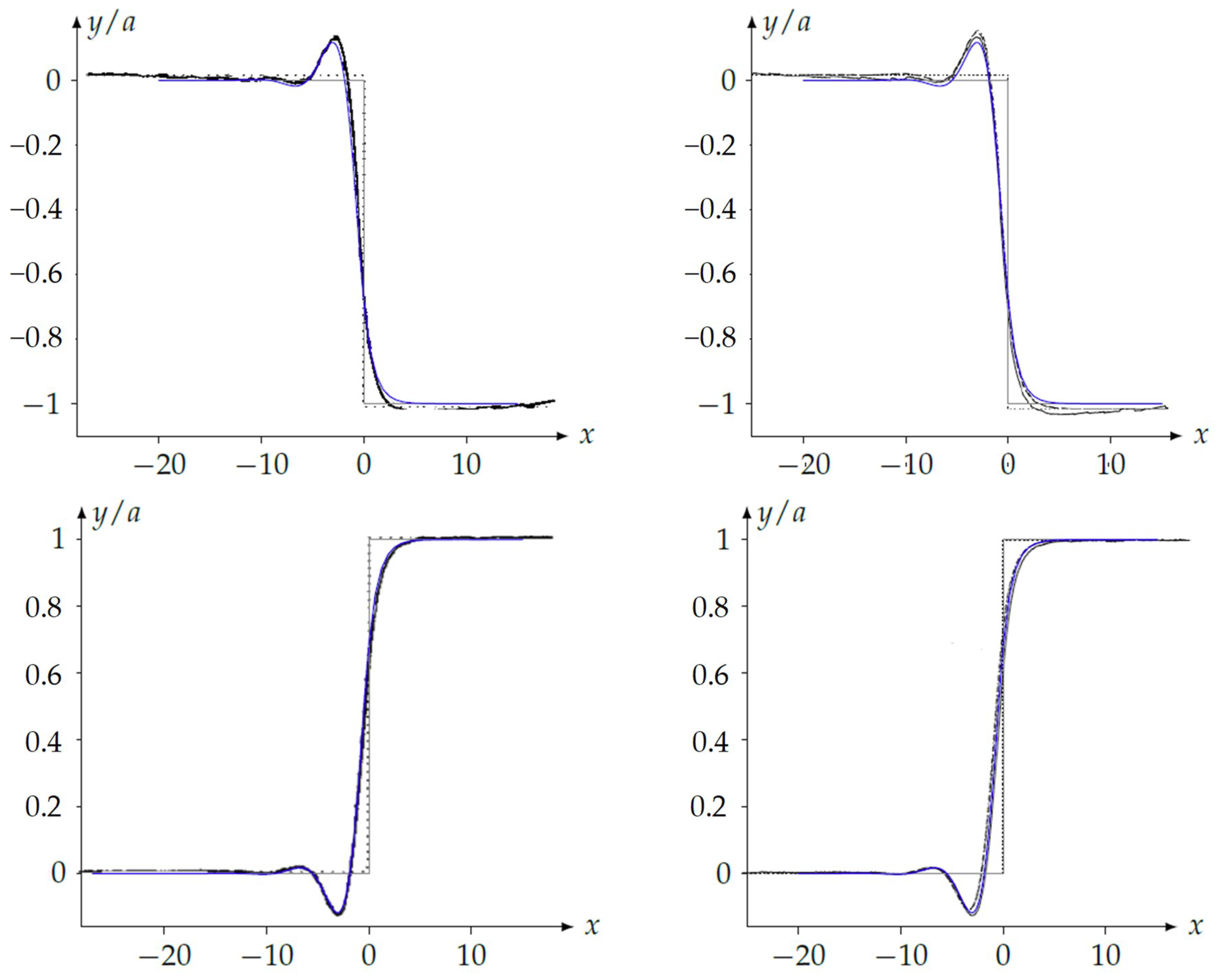
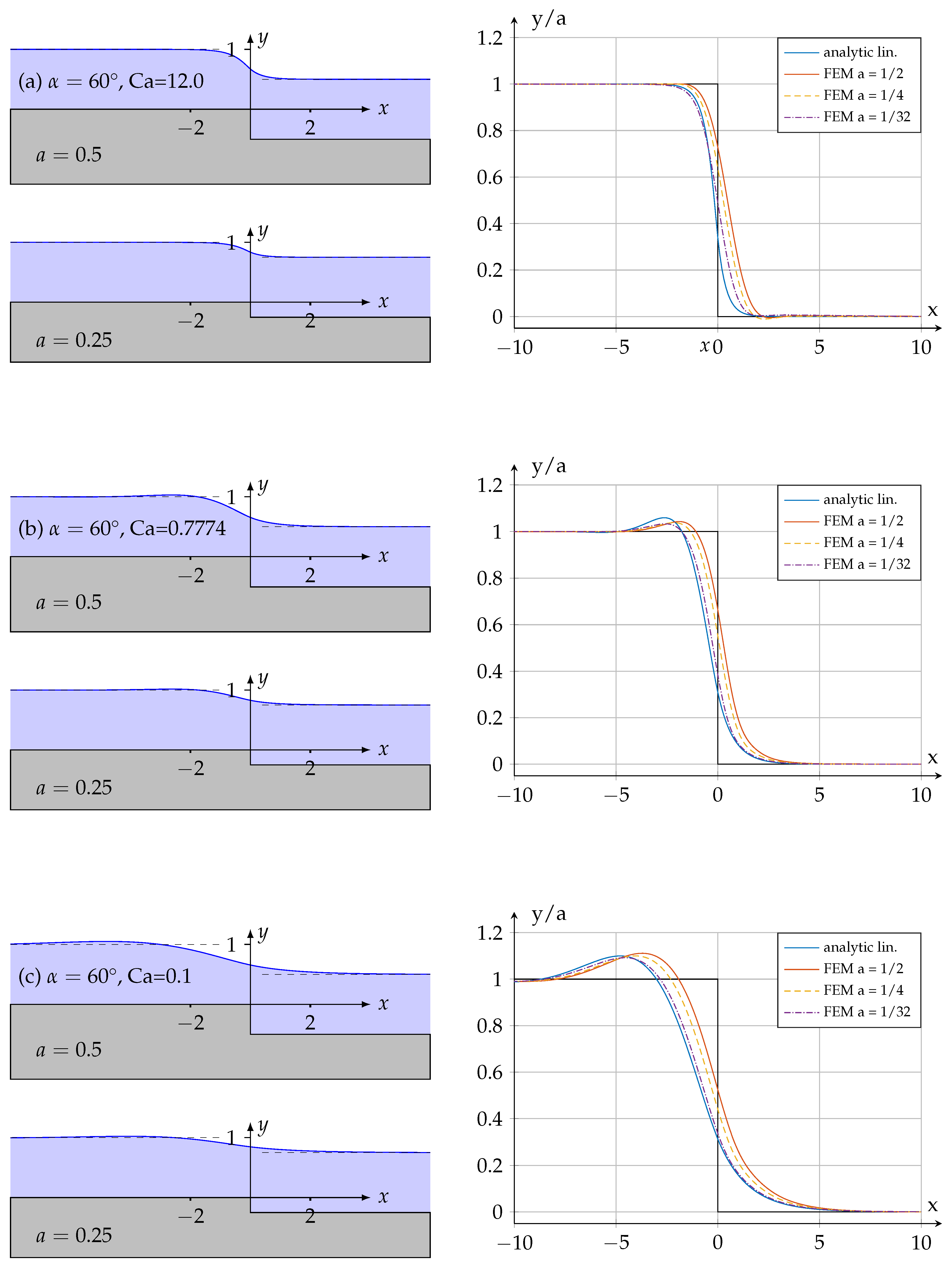
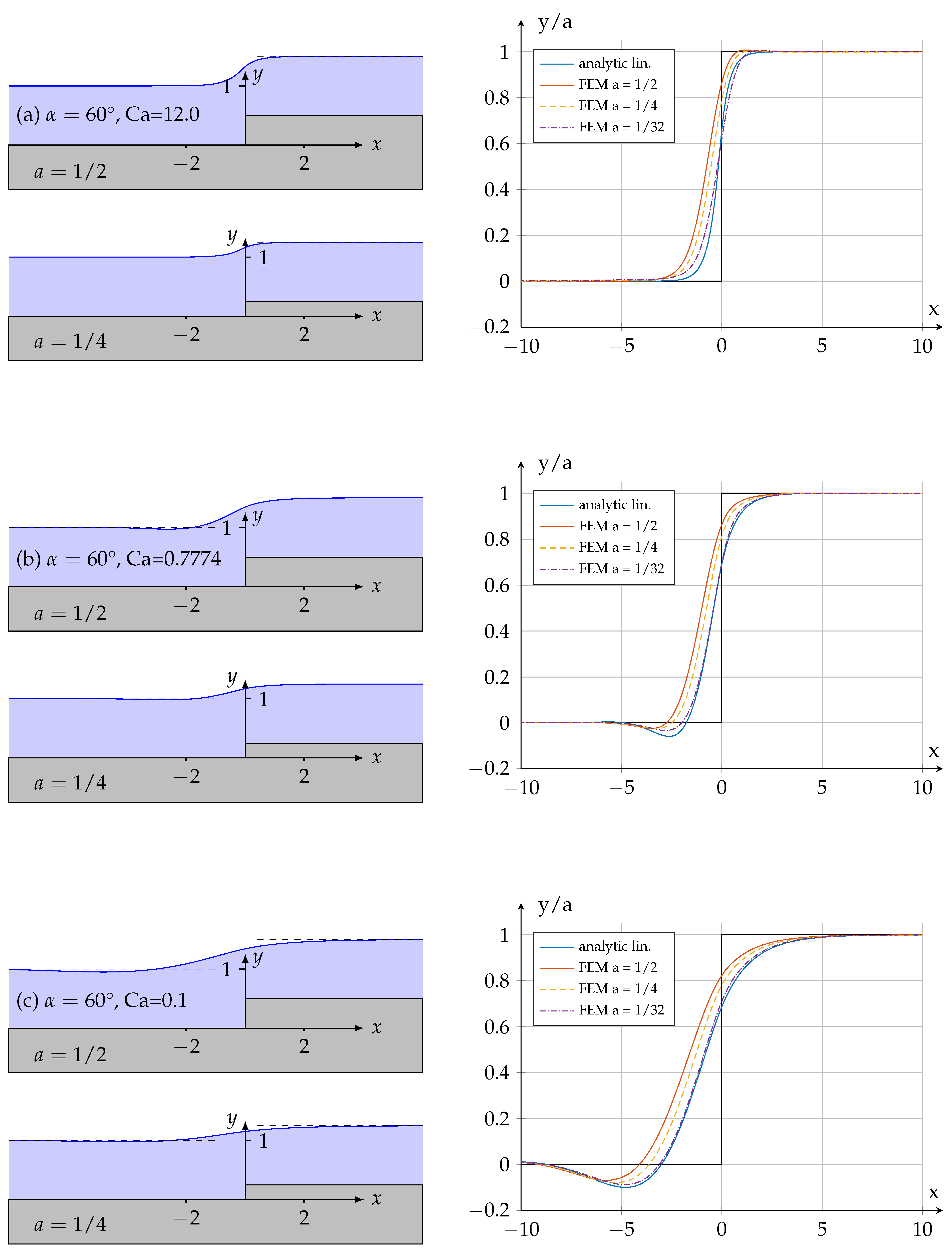
4.1. Step-Up and Step-Down Topography

Initially the linear approximation to the lubrication model derived in Section 3.2 was validated against existing experimental data and related numerical predictions available in the open literature, namely those of Decré and Baret [10] and Gaskell et al. [17], respectively, for film flow over step-up and step-down topography. The former still remain pretty much unique in the context of step-like topography while the latter have become a benchmark for such flows. Step-down and step-up topography is considered for the same set of parameter values and fluid properties: $\alpha =30$°, $a=0.2$ and $\mathrm{Ca}=7\times {10}^{-4}$. Figure 2 shows the free-surface disturbance predicted via equation (41) to be in excellent agreement for both configurations: the figures in the left column compare the linear solution (blue curve) against their experimental counterpart (dashed curve), while those in the right column compare the linear solution against both experiment and the numerical prediction (black curve) of [17]. Given the related experimental error involved [10] all three profiles can be said to agree extremely well.

Figure 3 shows the predicted free surface disturbance resulting from film flow down substrate containing a step-down topography, inclined at angle $\alpha =60$° to the horizontal, for step heights $a=1/2$, $1/4$ and $1/32$ for different values of $\mathrm{Ca}$ (12.0, 0.774 and 0.1). The entire flow regime, obtained using the linear model, is shown in the left column for $a=1/2$ and $1/4$; while in the right column only the predicted free surface profile (both analytic and FE) is presented for all three step heights. Using A as a alternative scaling length in the vertical direction, the analytically predicted profile becomes independent of a due to the linearity of the analytical approach, while the FEM solution of the full nonlinear problem clearly reveals a dependence of the surface profile on a, manifesting itself as a shift of the free surface in the upstream direction with decreasing a; such that for very small a the numerical solution approaches the analytical one. In such cases, agreement between the analytical and numerical solution is better still the smaller the Capillary number, since due to the stronger influence of surface tension the free surface disturbance is more gradual (smoother); which is a key requirement of the lubrication assumption.

For small surface tension ($\mathrm{Ca}=12$), case (a), the free surface height transitions monotonically from upstream to downstream. In contrast, for a Capillary number below a critical value for the chosen inclination angle (cases (b) and (c)), on the upstream side of the step the free surface experiences a maximum value, above that of the Nusselt thickness, before recovering to attain this asymptotic thickness at a distance upstream of the step dependent on the value of Ca. As expected, this capillary ridge is more pronounced for smaller values of Ca and is shifted further in the upstream direction.

Film flow over a step-up feature exhibits qualitatively similar behaviour but in this case, and in contrast, a capillary trough forms on the upstream side of the step. Equivalent plots to those for a step-down are shown in Figure 4. A trough is clearly visible for sufficiently small Capillary numbers and comparison of the analytical solution with the accompanying numerical results reveals once again a systematic shift of the film surface in one direction, this time downstream with decreasing a; the correspondence between the two becoming better for smaller a, and as observed in the case of a step-down the agreement between the two solutions is better still the smaller the Capillary number. Otherwise, overall good agreement between the analytical and numerical predictions is observed.

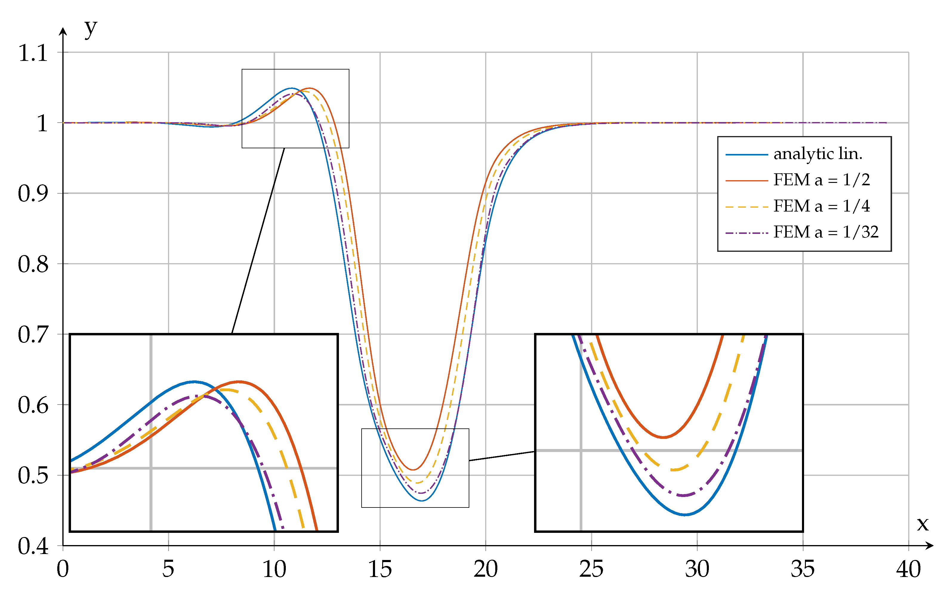
4.2. Trench Topography

In the left column of Figure 5 resulting free surface predictions, (61), for film flow over a trench topography, (60), are shown for the case $\alpha =80$°, with $a=1/2$, $\mathrm{Ca}=0.3$ and for different trench widths, ℓ. These are compared to corresponding FE solutions in the right column, the latter revealing also the internal flow structure in the form of streamlines.

In all cases, in the region spanning the side walls bounding the trench a distinct depression in the free surface is exhibited, the minimum of which shifts towards the step-up side of the trench with increasing ℓ, while on the upstream of the step-down a capillary ridge forms that overshoots the Nusselt film thickness before relaxing to this value further upstream. In the region $0\le x\le \ell$, for $\ell =2$ the local free surface position remains everywhere above a value equal to the unperturbed asymptotic film thickness, denoted by the horizontal dashed line; while for the wide trench, $\ell =6$, the minimum film thickness undershoots the value of $H_0$ in the middle of the tench.

The complementary FE results, shown in the right column of Figure 5, confirm these observations qualitatively revealing slight quantitative differences; the reason for the latter is arguably related to the vortical structures, or eddies, present in the corner regions of the trench formed by the side walls. It can be seen that the eddies are larger and extend further up the side of the trench, the smaller the value of ℓ. Since they occupy the space available in the trench proportionally, they shift the overlying flow and hence the free surface position in the vicinity of the trench, a feature that is not captured, for obvious reasons, using a lubrication approach. The analytically predicted local film thickness, depicted by the red curve, shows a broadening of the the free surface depression compared to the corresponding FE free surface streamline (the upper most blue curve). Nevertheless the expectation, based on the earlier investigations involving individual step-down and step-up features, is that agreement between the two will improve for smaller values of the depth parameter a. This is demonstrated quantitatively by a comparative study in terms of the predicted free surface profiles presented in Figure 6 based on, as used previously, an alternative scaling with respect to A and in which case the analytically obtained curves are independent of a.

Taking the third case presented in Figure 5 with a trench width $\ell =6$, capillary number $\mathrm{Ca}=0.3$, inclination angle $\alpha =80$° and $a=1/2$, as a starting point, reveals the broader analytically calculated free surface depression compared to the numerically computed one, which leads also to an overestimation of the maximum depression in the middle of the trench. However, it can be seen that as a is reduced, first to $a=1/4$ and then $a=1/32$, the quantitative difference between the predicted free surface profiles diminishes considerably, leading to very good agreement between two.

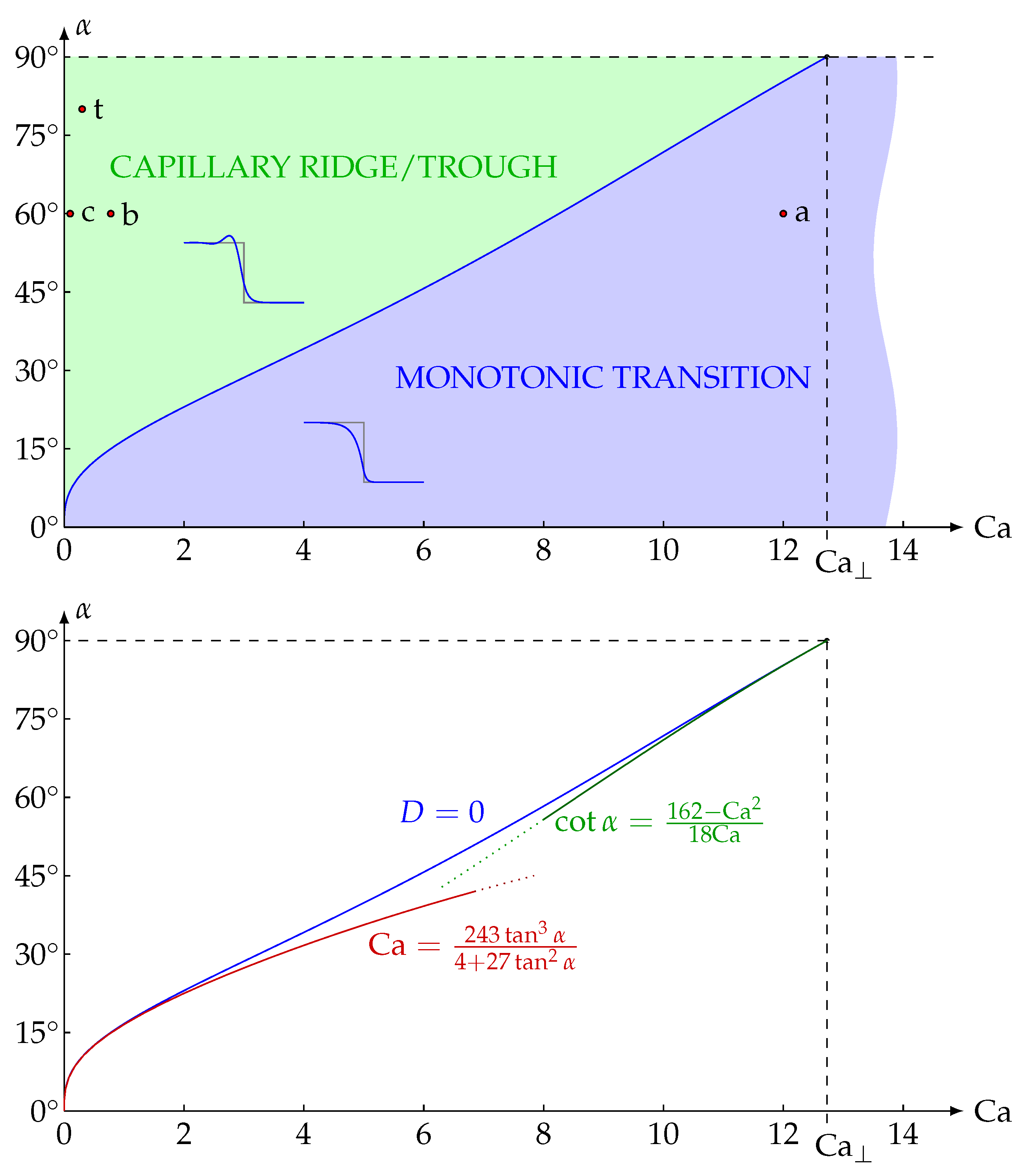
4.3. Capillary Criterion and Characteristic Free Surface Parameter Map

The dominant free surface disturbance (a capillary ridge or trough) present in the predictions of Figure 3, Figure 4, Figure 5 and Figure 6 for different values of $\alpha$ and Ca, raises the question as to whether a simple criterion can be found for identifying the appearance of such capillary-induced phenomena. As discussed earlier, the roots of the characteristic polynomial (39) are indicative in this respect: capillary ridges/troughs in tandem with a series of smaller strongly decaying oscillations occur if and only if two of its roots are complex, which is equivalent to inequality $D(\alpha ,\mathrm{Ca})>0$ for the discriminant (A18). Since D depends on $\alpha$ and Ca only, a characteristic parameter map in terms of these variables can be generated, as shown in the upper plot of Figure 7.

Accordingly, the regime that persists for a given $\alpha$ and increasing Ca, or vice versa, for the case of film flow over a piece-wise, step-like topography can be identified. The three different flow cases, (a)-(c), shown in Figure 3 and Figure 4 are identified on the map with the corresponding labels a-c; the point with the label t denoting the corresponding solution for the trench topography explored in Figure 5 and Figure 6. For a given $\alpha$ a capillary ridge/trough is only present below a critical Ca, the value of which is implicitly given by $D(\alpha ,\mathrm{Ca})=0$, becoming larger with increasing $\alpha$. The free surface profile inserts obtained analytically for the case of film flow over a step-down topography have been included to illustrate the distinction between the green region denoting the expected presence of a capillary ridge/trough, compared to the blue region signifying a monotonic transition; the locus of the curve $D(\alpha ,\mathrm{Ca})=0$ depicts the neutral, or aperiodic, limit separating the two regions. A striking feature is that even for a vertically aligned film ($\alpha =90$°) a finite critical capillary number Ca${}_{\perp }$ can be identified by solving $D(90°,{\mathrm{Ca}}_{\perp })=0$, giving Ca${}_{\perp }=9\sqrt{2}\approx 12.73$. For any capillary number above this value, the free surface can only transition monotonically in the direction of flow.

In Appendix A.5 explicit approximation formulae for the neutral limit curve for small inclination angles and those close to 90° are provided; the curves resulting from the latter are shown in the lower plot of Figure 7 in relation to the corresponding exact neutral limit curve.

5. Conclusions

It is shown that starting from a first integral of the NS equations, written in terms of the streamfunction $\mathsf{\Psi }$ and a potential $\mathsf{\Phi }$, is beneficial for investigating, from both a numerical and analytical standpoint, gravity-driven film flow down an inclined substrate featuring piece-wise planar step-like and trench topography. Using a least square FEM, the field equations and related boundary conditions can be solved without restrictions on Reynolds or Capillary number and substrate geometry. In tandem, a lubrication approximation of the first integral equations facilitates the modelling of such flows for zero Reynolds number when the height/depth of the topography is small compared to the overlying Nusselt film thickness. Reducing the problem to one requiring the solution of two nonlinear ODEs for the film thickness, which is shown to reproduce the degenerate Nusselt solution for film flow on a uniformly planar surface. Subsequent linearisation of these equations enables solutions to be found via a standard analytical approach, for the topographies of interest which once derived take a matter of seconds to obtain. For the case of step-down and step-up features they are shown to agree almost identically, for the same geometry and fluid properties, with the detailed experimental results of Decré and Baret [10] and the corresponding numerical predictions of Gaskell et al. [17].

Further detailed comparative studies concerning the free surface disturbance generated by step-like and trench topographies, including for the latter visualisation of the internal flow structure, confirm the closeness between corresponding analytic and FE predictions. As expected, better consistency between the two is reached for small values of topography height/depth compared to the asymptotic film thickness and when the value of the Capillary number is small. In all of the cases considered the analytical approach is found to provide an acceptable prediction of the resulting free surface disturbance.

A key result emerging from the adopted first first integral formulation, is the generation of a practically useful characteristic parameter map in terms of inclination angle of the substrate and the Capillary number, as demonstrated in Section 4.3. It allows instantaneous insight as to the behaviour of the free surface disturbance induced by capillary effects associated with a particular topographical feature: namely whether the feature gives rise to spacial oscillations exhibiting a dominant capillary ridge/trough or experiences a simple monotonic transition. A maximum value for the Capillary number, Ca${}_{\perp }=9\sqrt{2}\approx 12.73$, is identified above which the free surface disturbance will always transition monotonically. For Capillary number values below this upper bound the presence of spacial oscillations or otherwise, depends on the inclination angle only, with a clear demarkation between the two possibilities represented by a neutral limit curve. It is shown that approximate neutral limit curves can be derived which are in excellent agreement with the master curve both when Ca is small and tends towards the value Ca${}_{\perp }$. In some respects this parameter map plays a similar role to a typical stability map in which a curve of neutral stability separates regions of stable from an unstable film flow [30], and indeed from a wider perceptive an analogy with the problem of a buckling beam suggests itself.

Looking ahead, there is considerable scope for developing the methodology beyond the essentially linear approach used in the present work; numerical solution of the nonlinear ODE, (37), derived for the more general problem, offers the prospect of more accurate predictions of the free surface disturbance associated with film flow over topography other than simple piece-wise planar ones. The flexibility of the approach is such that it can be readily extended to include periodically repeating surface features, sharp or smooth, and to encompass the problem of film flow on curved 2D surfaces. Moreover, the recent 3D generalisation of the first integral approach reported by Scholle et al. [49] opens up the prospect of investigating film flows over 3D topographical features in a similar manner, again both analytically and numerically, and for extension to coating flows involving smooth 3D curved surfaces in general—for example film flow on a hemisphere as investigated by Takagi and Huppert [50].

References

1. Tabeling, P.; Chen, S. Introduction to Microfluidics; OUP Oxford: Oxford, UK, 2005. [Google Scholar]
2. Kang, B.; Lee, W.H.; Cho, K. Recent Advances in Organic Transistor Printing Processes. ACS Appl. Mater. Interfaces 2013, 5, 2302–2315. [Google Scholar] [CrossRef] [PubMed]
3. Müller, C.D.; Falcou, A.; Reckefuss, N.; Rojahn, M.; Wiederhirn, V.; Rudati, P.; Frohne, H.; Nuyken, O.; Becker, H.; Meerholz, K. Multi-colour organic light-emitting displays by solution processing. Nature 2003, 421, 829–833. [Google Scholar] [CrossRef] [PubMed]
4. Mandal, S.; Dell’Erba, G.; Luzio, A.; Bucella, S.G.; Perinot, A.; Calloni, A.; Berti, G.; Bussetti, G.; Duò, L.; Facchetti, A.; et al. Fully-printed, all-polymer, bendable and highly transparent complementary logic circuits. Org. Electron. 2015, 20, 132–141. [Google Scholar] [CrossRef]
5. Kistler, S.F.; Schweizer, P.M. Liquid Film Coating; Monographs and Studies in Mathematics; Chapman and Hall: New York, NY, USA, 1997. [Google Scholar]
6. Gaskell, P.H.; Jimack, P.K.; Sellier, M.; Thompson, H.M. Flow of evaporating, gravity-driven thin liquid films over topography. Phys. Fluids 2006, 18, 013601. [Google Scholar] [CrossRef]
7. Stillwagon, L.E.; Larson, R.G. Fundamentals of topographic substrate leveling. J. Appl. Phys. 1988, 63, 5251–5258. [Google Scholar] [CrossRef]
8. Stillwagon, L.E.; Larson, R.G. Leveling of thin films over uneven substrates during spin coating. Phys. Fluids A Fluid Dyn. 1990, 2, 1937–1944. [Google Scholar] [CrossRef]
9. Peurrung, L.M.; Graves, D.B. Spin coating over topography. IEEE Trans. Semicond. Manuf. 1993, 6, 72–76. [Google Scholar] [CrossRef]
10. Decré, M.M.; Baret, J.C. Gravity-driven flows of viscous liquids over two-dimensional topographies. J. Fluid Mech. 2003, 487, 147–166. [Google Scholar] [CrossRef]
11. Wierschem, A.; Pollak, T.; Heining, C.; Aksel, N. Suppression of eddies in films over topography. Phys. Fluids 2010, 22, 113603. [Google Scholar] [CrossRef]
12. Schörner, M.; Reck, D.; Aksel, N. Does the topography’s specific shape matter in general for the stability of film flows? Phys. Fluids 2015, 27, 042103. [Google Scholar] [CrossRef]
13. Oron, A.; Davis, S.H.; Bankoff, S.G. Long-scale evolution of thin liquid films. Rev. Mod. Phys. 1997, 69, 931–980. [Google Scholar] [CrossRef]
14. Gaskell, P.H.; Lee, Y.C.; Thompson, H.M. Thin film flow over and around surface topography: A general solver for the long-wave approximation and related equations. Comput. Model. Eng. Sci. 2010, 62, 77–112. [Google Scholar] [CrossRef]
15. Kalliadasis, S.; Bielarz, C.; Homsy, G.M. Steady free-surface thin film flows over topography. Phys. Fluids 2000, 12, 1889–1898. [Google Scholar] [CrossRef]
16. Mazouchi, A.; Homsy, G.M. Free surface Stokes flow over topography. Phys. Fluids 2001, 13, 2751–2761. [Google Scholar] [CrossRef]
17. Gaskell, P.H.; Jimack, P.K.; Sellier, M.; Thompson, H.M.; Wilson, M.C.T. Gravity-driven flow of continuous thin liquid films on non-porous substrates with topography. J. Fluid Mech. 2004, 509, 253–280. [Google Scholar] [CrossRef]
18. Veremieiev, S.; Thompson, H.M.; Lee, Y.C.; Gaskell, P.H. Inertial thin film flow on planar surfaces featuring topography. Comput. Fluids 2010, 39, 431–450. [Google Scholar] [CrossRef]
19. Hayes, M.; O’Brien, S.B.G.; Lammers, J.H. Green’s function for steady flow over a small two-dimensional topography. Phys. Fluids 2000, 12, 2845–2858. [Google Scholar] [CrossRef]
20. Scholle, M.; Haas, A.; Aksel, N.; Wilson, M.C.T.; Thompson, H.M.; Gaskell, P.H. Competing geometric and inertial effects on local flow structure in thick gravity-driven fluid films. Phys. Fluids 2008, 20, 123101. [Google Scholar] [CrossRef]
21. Blyth, M.G.; Pozrikidis, C. Film flow down an inclined plane over a three-dimensional obstacle. Phys. Fluids 2006, 18, 052104. [Google Scholar] [CrossRef]
22. Baxter, S.J.; Power, H.; Cliffe, K.A.; Hibberd, S. Three-dimensional thin film flow over and around an obstacle on an inclined plane. Phys. Fluids 2009, 21, 032102. [Google Scholar] [CrossRef]
23. Veremieiev, S.; Thompson, H.M.; Gaskell, P.H. Free-surface film flow over topography: Full three-dimensional finite element solutions. Comput. Fluids 2015, 122, 66–82. [Google Scholar] [CrossRef]
24. Heining, C.; Pollak, T.; Aksel, N. Pattern formation and mixing in three-dimensional film flow. Phys. Fluids 2012, 24, 042102. [Google Scholar] [CrossRef]
25. Ataki, A.; Bart, H.J. The Use of the VOF-Model to Study the Wetting of Solid Surfaces. Chem. Eng. Technol. 2004, 27, 1109–1114. [Google Scholar] [CrossRef]
26. Singh, R.K.; Galvin, J.E.; Sun, X. Three-dimensional simulation of rivulet and film flows over an inclined plate: Effects of solvent properties and contact angle. Chem. Eng. Sci. 2016, 142, 244–257. [Google Scholar] [CrossRef]
27. Singh, R.K.; Galvin, J.E.; Whyatt, G.A.; Sun, X. Breakup of a liquid rivulet falling over an inclined plate: Identification of a critical Weber number. Phys. Fluids 2017, 29, 052101. [Google Scholar] [CrossRef]
28. Trifonov, Y.Y. Stability of a viscous liquid film flowing down a periodic surface. Int. J. Multiph. Flow 2007, 33, 1186–1204. [Google Scholar] [CrossRef]
29. Pollak, T.; Aksel, N. Crucial flow stabilization and multiple instability branches of gravity-driven films over topography. Phys. Fluids 2013, 25, 024103. [Google Scholar] [CrossRef]
30. D’Alessio, S.J.D.; Pascal, J.P.; Jasmine, H.A. Instability in gravity-driven flow over uneven surfaces. Phys. Fluids 2009, 21, 062105. [Google Scholar] [CrossRef]
31. Argyriadi, K.; Vlachogiannis, M.; Bontozoglou, V. Experimental study of inclined film flow along periodic corrugations: The effect of wall steepness. Phys. Fluids 2006, 18, 012102. [Google Scholar] [CrossRef]
32. Nguyen, P.K.; Bontozoglou, V. Steady solutions of inertial film flow along strongly undulated substrates. Phys. Fluids 2011, 23, 052103. [Google Scholar] [CrossRef]
33. Schörner, M.; Reck, D.; Aksel, N.; Trifonov, Y. Switching between different types of stability isles in films over topographies. Acta Mech. 2018, 229, 423–436. [Google Scholar] [CrossRef]
34. Dauth, M.; Aksel, N. Breaking of waves on thin films over topographies. Phys. Fluids 2018, 30, 082113. [Google Scholar] [CrossRef]
35. Veremieiev, S.; Wacks, D.H. Modelling gravity-driven film flow on inclined corrugated substrate using a high fidelity weighted residual integral boundary-layer method. Phys. Fluids 2019, 31, 022101. [Google Scholar] [CrossRef]
36. Sellier, M. Substrate design or reconstruction from free surface data for thin film flows. Phys. Fluids 2008, 20, 062106. [Google Scholar] [CrossRef]
37. Heining, C.; Pollak, T.; Sellier, M. Flow domain identification from free surface velocity in thin inertial films. J. Fluid Mech. 2013, 720, 338–356. [Google Scholar] [CrossRef]
38. Sellier, M. Inverse problems in free surface flows: A review. Acta Mech. 2016, 227, 913–935. [Google Scholar] [CrossRef]
39. Saprykin, S.; Koopmans, R.J.; Kalliadasis, S. Free-surface thin-film flows over topography: Influence of inertia and viscoelasticity. J. Fluid Mech. 2007, 578, 271–293. [Google Scholar] [CrossRef]
40. Veremieiev, S.; Thompson, H.M.; Scholle, M.; Lee, Y.C.; Gaskell, P.H. Electrified thin film flow at finite Reynolds number on planar substrates featuring topography. Int. J. Multiph. Flow 2012, 44, 48–69. [Google Scholar] [CrossRef]
41. Papageorgiou, D.T. Film Flows in the Presence of Electric Fields. Ann. Rev. Fluid Mech. 2019, 51, 155–187. [Google Scholar] [CrossRef]
42. Ranger, K.B. Parametrization of general solutions for the Navier-Stokes equations. Q. J. Appl. Math. 1994, 52, 335–341. [Google Scholar] [CrossRef]
43. Coleman, C.J. On the use of complex variables in the analysis of flows of an elastic fluid. J. Non-Newtonian Fluid Mech. 1984, 15, 227–238. [Google Scholar] [CrossRef]
44. Scholle, M.; Haas, A.; Gaskell, P.H. A first integral of Navier-Stokes equations and its applications. Proc. R. Soc. 2011, A467, 127–143. [Google Scholar] [CrossRef]
45. Marner, F.; Gaskell, P.H.; Scholle, M. On a potential-velocity formulation of Navier-Stokes equations. Phys. Mesomech. 2014, 17, 341–348. [Google Scholar] [CrossRef]
46. Marner, F. Potential-Based Formulations of the Navier-Stokes Equations and Their Application. Ph.D. Thesis, Durham University, Durham, UK, 2019. [Google Scholar]
47. Bochev, P.B.; Gunzburger, M.D. Least-Squares Finite Element Methods; Applied Mathematical Sciences, Volume 166; Springer: New York, NY, USA, 2009. [Google Scholar]
48. Veremieiev, S. Gravity-Driven Continuous Thin Film Flow over Topography. Ph.D. Thesis, University of Leeds, Leeds, UK, 2011. [Google Scholar]
49. Scholle, M.; Gaskell, P.H.; Marner, F. Exact integration of the unsteady incompressible Navier-Stokes equations, gauge criteria, and applications. J. Math. Phys. 2018, 59, 043101. [Google Scholar] [CrossRef]
50. Takagi, D.; Huppert, H.E. Flow and instability of thin films on a sphere. J. Fluid Mech. 2009, 647, 221–238. [Google Scholar] [CrossRef]
51. Selby, S.M. CRC Standard Mathematical Tables, 23rd ed.; CRC Press: Boca Raton, FL, USA, 1975. [Google Scholar]
Figure 1. Schematic of a continuous film of liquid, asymptotic thickness H 0 , flowing down a rigid piece-wise planar substrate, b ˜ ( X ) , inclined at angle α to the horizontal and containing, for illustration purposes, a sharp trench topography, height A and length L; shown also is the orientation of the corresponding ( X , Y ) co-ordinate system, with f ˜ ( X ) denoting the shape of the free surface disturbance experienced by the film.
Fluids 04 00082 g001
Figure 2. Comparison of the free surface disturbance predicted by (41) (blue curve) against the experimental data (dashed curve) of [10] (left column) as well as the numerical solution (black curve) of Gaskell et al. [17] (right column), both for a step-down (top row) and a step-up (bottom row) topography: the flow is from left to right with α = 30 °, and Ca = 7 × 10 4 and the dotted line shows the associated nature of the topography for comparison purposes.
Fluids 04 00082 g002
Figure 3. Linearised lubrication model solutions (left column) for film flow over a step-down ( a = 1 / 2 , 1 / 4 and 1 / 32 for different values of Ca (12.0 (top), 0.7774 (middle), 0.1 (bottom)) and α = 60 ° ) showing the predicted free surface disturbance (blue curve), compared with FE solutions of the first integral equations (right column; using a different scaling for clarity): (a) monotonic transition; (b,c) damped spatial oscillations upstream. The flow is from left to right, the dashed lines in the left-hand column indicating the unperturbed film thickness on the upstream and downstream sides of the step.
Fluids 04 00082 g003
Figure 4. Linearised lubrication model solutions (left column) for film flow over a step-up ( a = 1 / 2 , 1 / 4 and 1 / 32 for different values of Ca (12.0 (top), 0.7774 (middle), 0.1 (bottom)) and α = 60 ° ) showing the predicted free surface disturbance (blue curve), compared with FE solutions of the first integral equations (right column; using a different scaling for clarity): (a) monotonic transition; (b,c) damped spatial oscillations upstream. The flow is from left to right, the dashed lines in the left-hand column indicating the unperturbed film thickness on the upstream and downstream sides of the step.
Fluids 04 00082 g004
Figure 5. Predicted free surface disturbance for film flow over a trench topography ( α = 80 °, a = 1 / 2 and Ca = 0.3 for different trench widths : 2 (top); 4 (middle); 6 (bottom)), obtained analytically (left column) and numerically (right column); in the latter the blue free surface streamline represents the steady-state FE solution of the first integral equations with the red curve indicating the corresponding free surface shape obtained from the linear theory. The flow is from left to right with the dashed lines indicating the equivalent corresponding asymptotic film thickness, H 0 , upstream of and in the middle of the trench.
Fluids 04 00082 g005
Figure 6. A comparison of analytically and numerically predicted free surface profiles for film flow over a trench (located between x = 17 and x = 23 ) with α = 80 , Ca = 0.3 , = 6 for varying trench depth a. The superimposed inserts are magnified by a factor 2.5 .
Fluids 04 00082 g006
Figure 7. Upper plot: characteristic parameter map for α against Ca identifying the regions associated with (i) a monotonic transition of the free surface disturbance (blue region) and (ii) the occurrence of spatial oscillations with a dominant capillary ridge/trough (green region); the two regions being separated by a neutral limit curve along which the discriminant (A18) vanishes. The different step-up/-down cases, (a)-(c), explored in Figure 3 and Figure 4 are identified by the labels a-c, respectively, the trench case considered in Figure 5 and Figure 6 by the label t. Lower plot: Neutral limit curve (blue curve) compared with the corresponding curves obtained using the approximations (A26) and (A27), derived in Appendix A.5, when α is small (red curve) and close to 90° (green curve), respectively.
Fluids 04 00082 g007