Article

Onset of Convection in an Inclined Anisotropic Porous Layer with Internal Heat Generation

by
Leiv Storesletten
1 and
D. Andrew S. Rees
2,*
1
Department of Mathematics, University of Agder, Serviceboks 422, 4604 Kristiansand, Norway
2
Department of Mechanical Engineering, University of Bath, Bath BA2 7AY, UK
*
Author to whom correspondence should be addressed.
Fluids 2019, 4(2), 75; https://doi.org/10.3390/fluids4020075
Submission received: 20 March 2019 / Revised: 10 April 2019 / Accepted: 11 April 2019 / Published: 16 April 2019
(This article belongs to the Special Issue Convective Instability in Porous Media, Volume II)

Abstract

:
The onset of convection in an inclined porous layer which is heated internally by a uniform distribution of heat sources is considered. We investigate the combined effects of inclination, anisotropy and internal heat generation on the linear instability of the basic parallel flow. When the Rayleigh number is sufficiently large, instability occurs and a convective motion is set up. It turns out that the preferred motion at convection onset depends quite strongly on the anisotropy ratio, ξ , and the inclination angle. When ξ < 1 the preferred motion is in the form of longitudinal rolls for all inclinations. When ξ > 1 transverse rolls are preferred for small inclinations but, at high inclinations, longitudinal rolls are preferred. At intermediate inclinations the preferred roll orientation varies smoothly between these two extremes.

1. Introduction

The onset of convection in porous layers forms one of the classical problems of stability theory and the most well-known of these is the the Darcy-Bénard (or Horton-Rogers-Lapwood) problem [1,2]. In its simplest form a horizontal porous layer for which Darcy’s law applies has a lower boundary which is impermeable and uniformly hot while the impermeable upper boundary is uniformly cold. It is well-known that the critical Darcy-Rayleigh number for the onset of convection is 4 π 2 when the layer is unbounded horizontally. The corresponding wavenumber is π . A second well-known problem of the same type comprises a porous layer with uniformly cold boundaries but which is heated via a uniform internal heat generation mechanism. Practical examples of such systems include heat removal from fuel debris in nuclear reactors, the underground disposal of radioactive waste materials, agricultural applications involving the storage of foodstuff, and exothermic chemical reactions in packed-bed reactors. It is this configuration which we study here and we shall determine the combined effects of layer inclination and anisotropy on the onset of convection.
The first experimental and theoretical studies on the topic of an internally-heated layer were undertaken in the late 1970s by Kulacki and Ramchandani [3], Gasser and Kazimi [4], Buretta and Berman [5], Hardee and Nilson [6], Hwang and Marr [7], Tveitereid [8], Rhee et al. [9] and Kulacki and Freeman [10]. These papers represent quite a wide range of different types of boundary condition such as a free upper surface in [4] or the presence of an insulated bounding surface [8,10]. The case where both surfaces are impermeable and are at identical constant temperatures has a critical Darcy-Rayleigh number of 471.38 and a critical wavenumber of 4.6752, values which have been obtained by various authors such as Barletta et al. [11], Nandal and Mahajan [12] and Nouri-Borujerdi et al. [13,14]. This ten-fold rise in the critical Darcy-Rayleigh number may be explained at least qualitatively by the facts that (i) the internally-heated case admits a destabilising temperature gradient only in the upper half of the layer and (ii) the maximum temperature difference is only 1 8 of that of that of the classical Darcy-Bénard layer. The increase in the wavenumber may be traced to the fact that convection cells tend to remain of roughly a unit aspect ratio, and given that most of the disturbance occuies the upper half of the layer its horizontal period is reduced from that of the Darcy-Bénard problem.
Many authors have considered different extensions to this ‘pure’ internally-heated problem as described above. Nield and Kuznetsov [15] considered different types of nonuniform internal heating profiles, while Nield and Kuznetsov [16] and Kuznetsov and Nield [17] studied the effects of inhomogeneity in the structure of the porous medium itself. Matta and Hill [18], on the other hand, considered an equivalent double-diffusive configuration where the heat source depends on the solutal concentration. Nouri-Borujerdi et al. [13] considered the equivalent Darcy-Brinkman case and the critical Darcy-Rayleigh number was found to rise as the Darcy number increases. Nouri-Borujerdi et al. [14] relaxed the assumption of local thermal equilibrium between the phases. In addition Mahajan and Nandal [19] considered how anisotropy and Brinkman effects alter the stability criteria, while Yadav et al. [20] consider the combined effects of rotation and the Brinkman terms. We also mention some works which include anisotropy but with heating from below: Malashetty and Swamy [21] and Yavogan et al. [22] both analysed the effect of a viscoelastic fluid and obtained an analytical expression for the critical Darcy-Rayleigh number, Raghunatha et al. [23] considered the case when the porous medium is saturated by an Oldroyd-B fluid, Abdelhafez and Tsybulin [24] who considered the presence of a binary fluid, Yadav and Kim [25] who studied the instability of a time-evolving boundary layer flow and Storesletten and Rees [26] on the instability of a boundary layer induced by uniform surface suction.
The present paper consists of a linear stability analysis of the above-described uniformly-heated porous layer, but we also consider the extra effects of anisotropy and inclination. It is well-known from studies of the Darcy-Bénard problem that the introduction of anisotropy by the modification of one of the principal permeabilities in the horizontal direction removes the directional invariance of the roll pattern to one where there is a preferred direction. Thus if the y-direction is vertical and the altered permeability is in the x-direction, then the axis of resulting rolls will be in the x-direction if the permeability in the x-direction is larger than the other principal permeabilities, and in the z-direction otherwise. The effect of inclination on the Darcy-Bénard problem is to cause longitudinal rolls, i.e., those with axes up the layer, to be preferred. The combination of these two effects, especially when they conflict with regard to their prediction of the preferred roll direction, is of some great interest. In this regard the works by Rees and Postelnicu [27], Postelnicu and Rees [28] and Rees et al. [29] are important for they display both sudden and smooth transitions in the preferred roll direction as the inclination is increased.
This work, then, represents the combined effects of internal heating, anisotropy and inclination. It may be regarded as being an extension (i) of the works of Rees and Postelnicu [27] and Storesletten and Tveitereid [29] by having the presence of internal heating, (ii) of the work of Barletta et al. [11] by the inclusion of the effect of anisotropy and (iii) of the works of Mahajan and Nandal [19] and Capone et al. [30] by inclining the layer. We concentrate first on two-dimensional convection (transverse rolls) which will always arise whenever the porous layer is sufficiently narrow in the spanwise direction. Then we consider rolls of all orientations, the ultimate aim being to determine how the critical orientation varies with the governing parameters, namely the anisotropy ratio, ξ , and the inclination angle, ϕ .

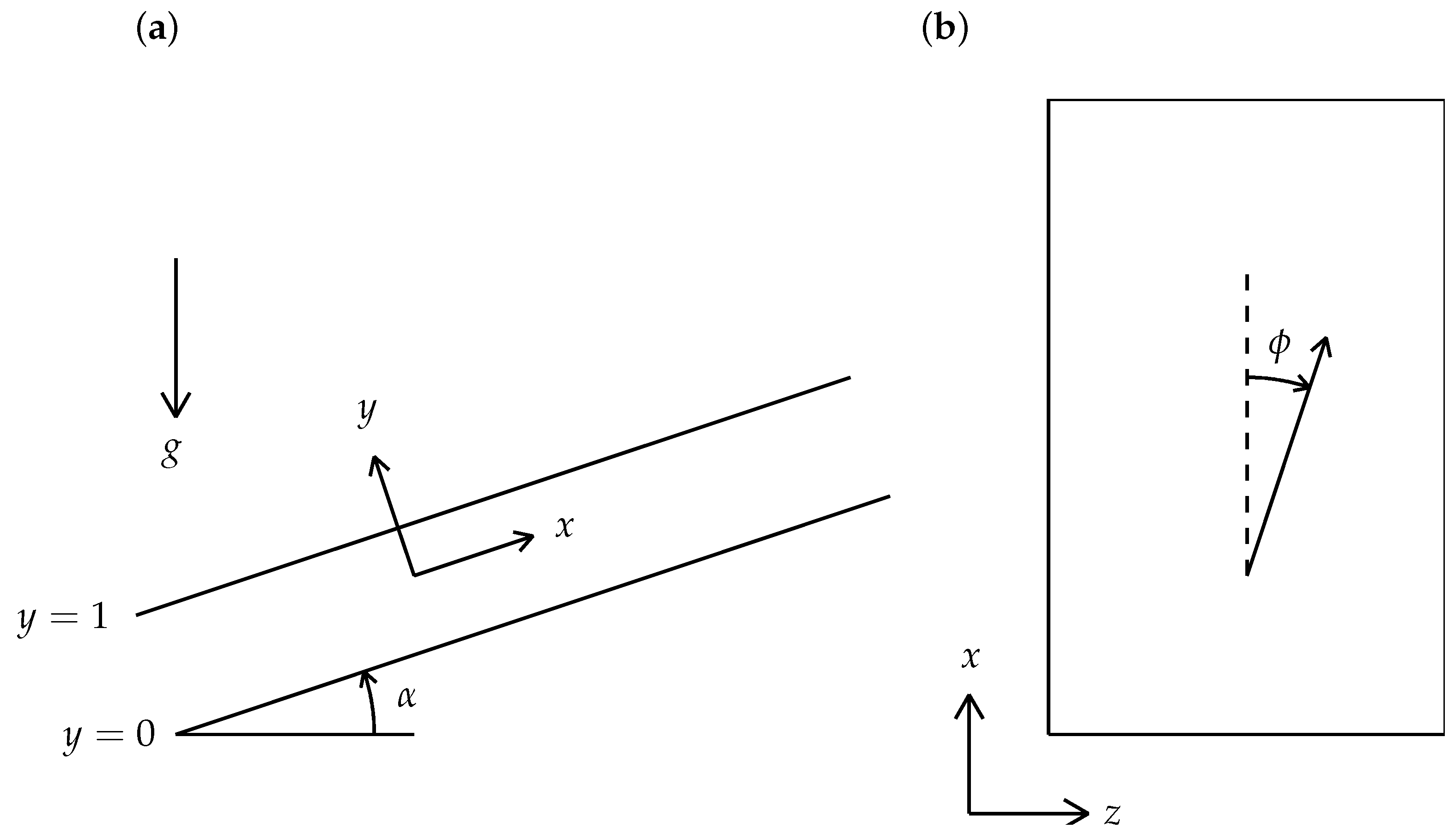
2. Governing Equations and the Basic State

We consider the onset of convection in an inclined porous layer of infinite lateral extent which is heated internally by a uniform distribution of heat sources. The layer is bounded by two parallel solid plates which are separated by a distance h and inclined at an angle α to the horizontal. Both boundaries are held at a constant temperature T 0 . The horizontal z-axis forms the direction about which the layer has been rotated, the y-axis is perpendicular to the bounding plates, and the x-axis lies in the lower surface pointing up the plane. The detailed configuration is shown in Figure 1. Moreover, the anisotropic porous layer is taken to be transversely isotropic in the permeability but homogenously isotropic in the thermal diffusivity. The saturating fluid is assumed to be such that Darcy’s law holds and the Oberbeck-Boussinesq approximation is valid. The governing equations are then,
u x + v y + w z = 0 ,
u = K L μ p x + ρ 0 g β ( T T 0 ) sin α ,
v = K T μ p y + ρ 0 g β ( T T 0 ) cos α ,
w = K T μ p z ,
σ T t + u T x + v T y + w T z = κ 2 T + q k m ,
where q is the rate of heat generated within the porous medium per unit volume, β is the coefficient of cubical expansion, k m is the thermal conductivity of the porous medium, and p is the pressure, which includes the hydro-static pressure. Terms in Equations (1)–(5) have their usual meaning in the porous medium context, but we mentioned that K L is the permeability in the x-direction, K T is the permeability in both the y- and z-directions, that σ is the heat capacity ratio, and κ is the thermal diffusivity. A zero subscript denotes reference quantities. Further details are in the Abbreviations at the end of the paper. The variables are made dimensionless by setting
( x , y , z ) = h ( x , y , z ) , ( u , v , w ) = κ h ( u , v , w ) ,
T T 0 = q h 2 k m θ , p = κ μ K T p , t = σ h 2 κ t ,
so that the governing equations reduce to,
u x + v y + w z = 0 ,
u = ξ p x + ξ Ra θ sin α , v = p y + Ra θ cos α , w = p z ,
θ t + u θ x + v θ y + w θ z = 2 θ + 1 .
The dimensionless parameters which appear in these equations are the Darcy-Rayleigh number, Ra , and the anisotropy parameter, ξ , which are given respectively by,
Ra = ρ 0 g β K T h κ μ q h 2 k m , ξ = K L K T .
In this paper we shall use two different formulations of the governing equations for the numerical work. In the first instance two-dimensional cases will be considered using the streamfunction/temperature approach whereas for three-dimensional flows a pressure/temperature approach will be used. In the former case the streamfunction is defined using
u = ψ y , v = ψ x , w = 0 ,
and therefore Equation (8) is satisfied while Equations (9) and (10) transform into,
ξ 2 ψ x 2 + 2 ψ y 2 = ξ Ra θ x cos α θ y sin α ,
θ t = 2 θ x 2 + 2 θ y 2 + ψ y θ x ψ x θ y + 1 .
In the latter case ( u , v , w ) may be eliminated from Equations (8)–(10) and we obtain the following governing equations for the unsteady flow:
ξ 2 p x 2 + 2 p y 2 + 2 p z 2 = Ra ξ θ x sin α + θ y cos α ,
θ t + Ra θ ξ θ x sin α + θ y cos α ξ p x θ x + p y θ y + p z θ z = 2 θ x 2 + 2 θ y 2 + 2 θ z 2 + 1 .
For these two formulations we may write the boundary conditions in the form,
ψ = p y = θ = 0 on both y = 0 and y = 1 .
There exists a unique steady basic flow, v = ( u b , 0 , 0 ) , ψ = ψ b ( y ) , θ = θ b ( y ) and p = p b ( y ) where the net mass flux through a cross section x = constant is zero. This steady flow with nonlinear velocity and temperature profiles is given by,
u b = ξ Ra ( 1 2 y 2 + 1 2 y 1 12 ) sin α , ψ b = ξ Ra ( 1 6 y 3 1 4 y 2 + 1 12 y ) sin α ,
θ b = 1 2 ( y y 2 ) , p b = Ra [ 1 12 x sin α + ( 1 4 y 2 1 6 y 3 ) cos α ] + p 0 ,
where p 0 is the pressure at ( x , y , z ) = ( 0 , 0 , 0 ) .

3. Linear Stability Analysis for Two-Dimensional Disturbances

3.1. Reduction to ODE Eigenvalue Form

The linear stability characteristics of the basic steady state given by Equations (18) and (19) may be investigated by setting,
ψ = ψ b + ψ 1 , θ = θ b + θ 1 ,
where ψ 1 and θ 1 are asymptotically small perturbations in the streamfunction and temperature, respectively. The substitution of the expressions (20) into the governing Equations (13) and (14) followed by linearisation yields the following set of perturbation equations,
ξ 2 ψ 1 x 2 + 2 ψ 1 y 2 = ξ Ra θ 1 x cos α θ 1 y sin α ,
2 θ 1 x 2 + 2 θ 1 y 2 = 1 2 y ψ 1 x ξ Ra sin α 1 12 1 2 y + 1 2 y 2 θ 1 x + θ 1 t ,
which are to be solved subject to homogeneous Dirichlet conditions. The disturbances may be reduced to ordinary differential form by factoring out a monochromatic horizontal component: we let,
ψ 1 θ 1 = e i k x + λ t i Ψ ( y ) Θ ( y ) + complex conjugate .
Hence the disturbance equations reduce to,
Ψ ξ k 2 Ψ = ξ Ra k Θ cos α + i Θ sin α ,
Θ k 2 Θ = ( 1 2 y ) k Ψ i k ξ Ra sin α 1 12 1 2 y + 1 2 y 2 Θ + λ Θ ,
and the boundary conditions are that,
Ψ = Θ = 0 on both y = 0 and y = 1 .
This system may be regarded as an eigenvalue problem for the complex growth rate, λ , as a function of k, ξ , Ra and α . Alternatively, if we let λ = λ r + i λ i and set λ r = 0 to model marginal stability, then this system may instead be regarded as an eigenvalue problem for both the Darcy-Rayleigh number, Ra , and for λ i as functions of k, ξ and α .
We may now define the phase velocity of the disturbances by modifying the exponential in Equation (23). At marginal stability λ = i λ i and therefore,
e i k x + λ t = e i k ( x c t ) where c = λ i / k .

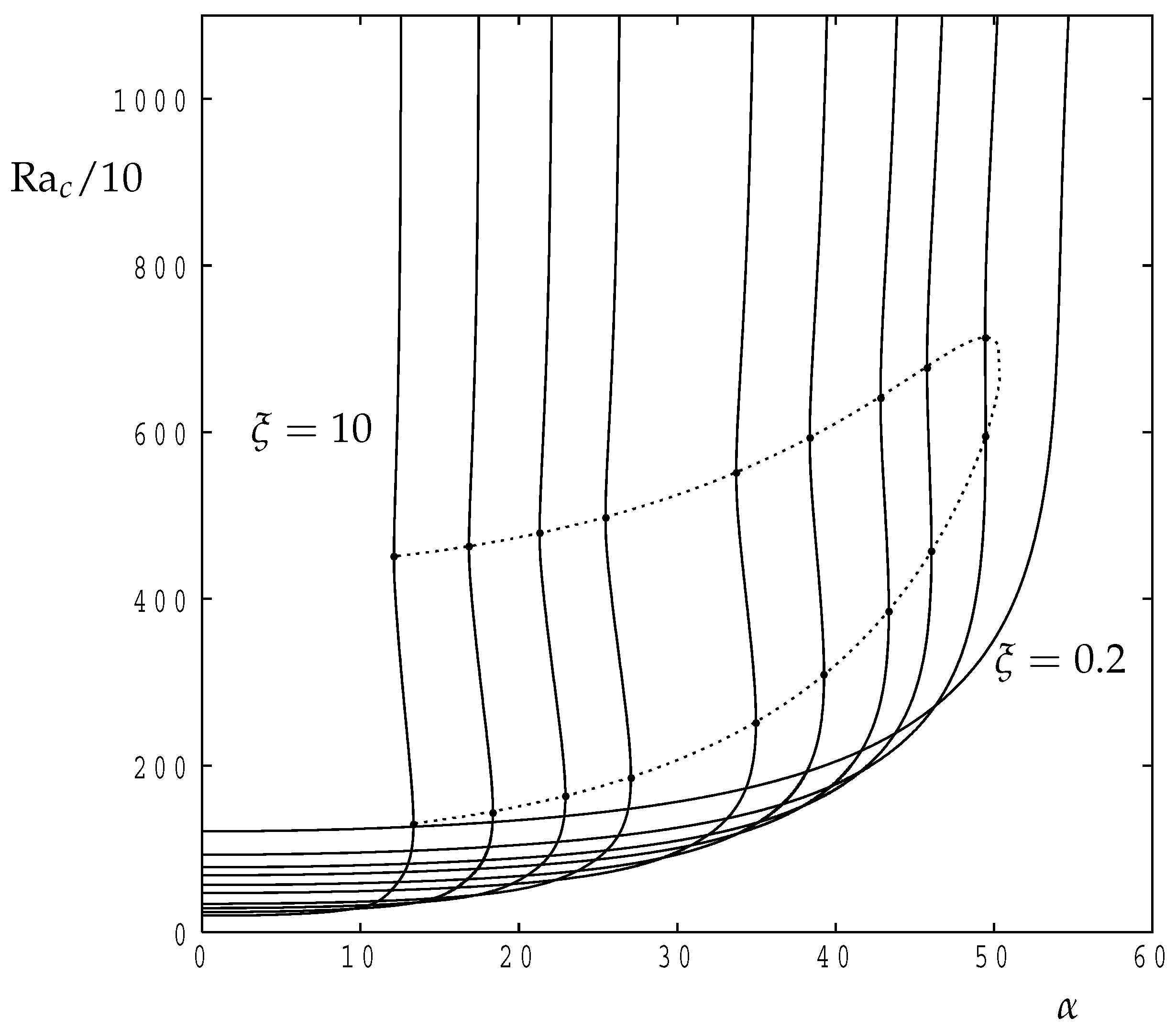
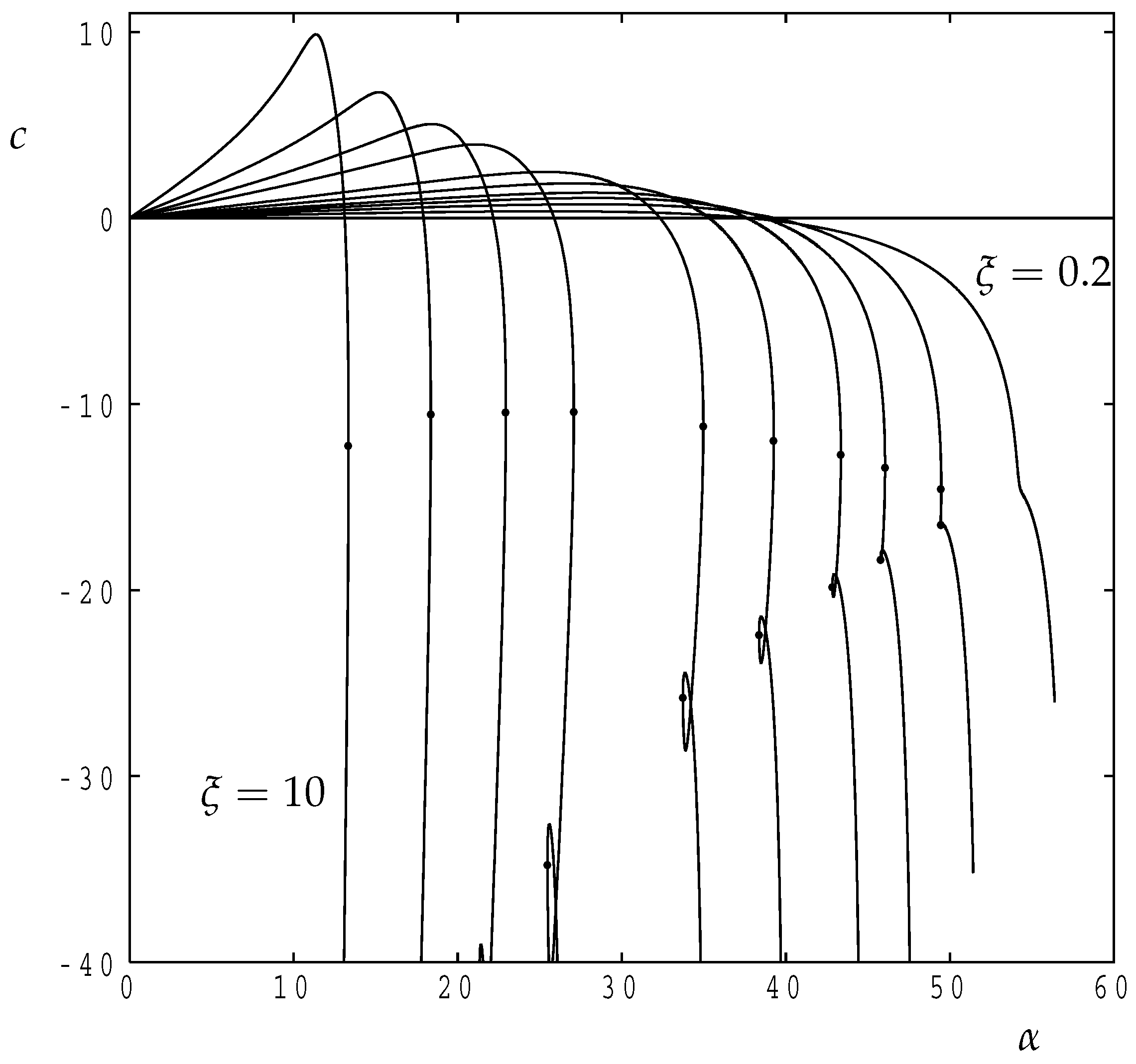
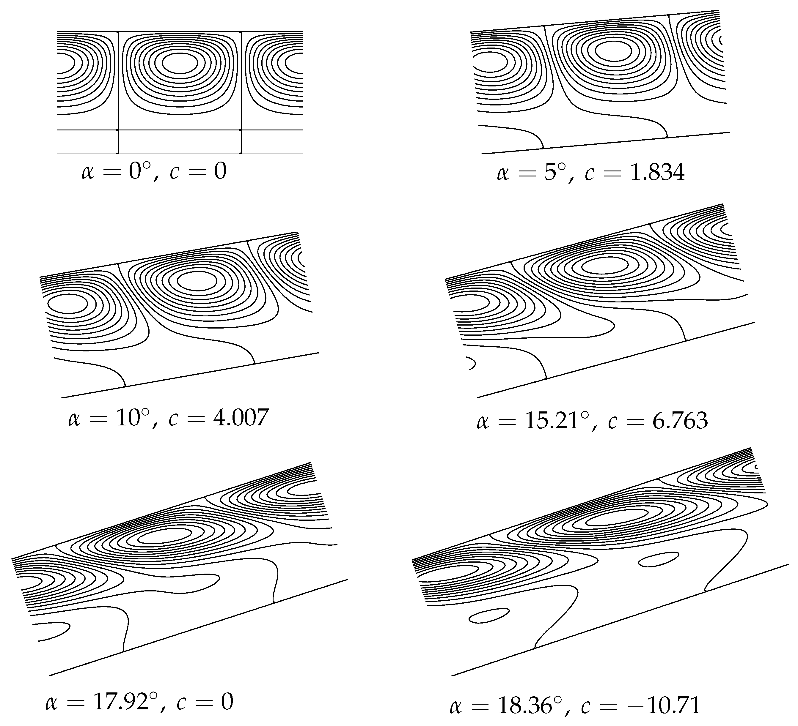
3.2. Numerical Results

In the first instance Equations (24)–(26) were discretised using second order accurate central difference approximations and the resulting difference equations were rearranged into a complex matrix eigenvalue problem for λ precisely in the manner described in Rees and Bassom [31]. For a chosen pair of values of ξ and inclination, α , the first few eigenvalues for λ were computed on a fine grid of values of Ra and k, and contours of λ r = 0 were plotted to provide the neutral curves. The use of N = 10 intervals in the range 0 y 1 gave poor results particularly when Ra or k was too large. The number of intervals was then increased first to N = 20 , then to N = 40 and ultimately to N = 80 , we found that, that the neutral curves presented in Figure 2 and which correspond to N = 40 exhibit no visual changes when comparing them with N = 80 solutions.
In more detail, Figure 2 displays four sets of neutral curves for ξ = 5 , 2, 0.5 and 0.2 . For this set of values of ξ the various frames of Figure 2 display the manner in which the neutral curves evolve as α increases in 1 increments from the horizontal case, α = 0 . For ease of comparison each subfigure corresponds to k and Ra lying in the ranges, 0 k 3 k c and 0 Ra 12 Ra c where k c and Ra c are the critical wavenumber and Darcy-Rayleigh number when the layer is horizontal ( α = 0 ). We have plotted the neutral curves corresponding to the first two modes.
It is clear from Figure 2 that the general form taken by the neutral curves remains almost unchanged as ξ varies. Thus the critical values of Ra (which correspond to the minimum of each neutral curve and which are labelled as Ra c hereinafter) always increase as the inclination, α , increases and this may be expected given that buoyancy decreases with increasing inclination. For three of the cases shown in Figure 2 there is a local maximum inclination angle which is at an isola point (shown as black disks). These points are characterised by being surrounded by elliptic-shaped neutral curves where the ξ = 2 case provides a good example since the value of α at the isola itself lies just above 27 . In these three cases ( ξ = 5 , 2 and 0.5 ) there also exists a saddle point; for ξ = 0.5 this is depicted as a red disk but the saddle points for ξ = 5 and ξ = 2 lie above the maximum value of Ra used for plotting.
Figure 3 gives an alternative view which both summarises and extends the above discussion and shows, for a wide selection of values of ξ , how the local minimum and maximum of Ra on each neutral curve varies with inclination. The lower set of black disks and the associated dotted curve correspond to how the value of Ra for the isolae varies with inclination, and the upper set correspond to the saddle points. These two curves eventually merge when ξ is roughly 0.27843 , which is in accord with the fact that no isola is displayed in Figure 2 for ξ = 0.2 . We presume that each of the solid curves shown in Figure 3 tend asymptotically toward a constant value of α as Ra c , as was shown in Rees and Bassom [31] for the inclined Darcy-Bénard problem.
Some indication of how the critical wavenumber varies with α may be gleaned from Figure 2, but a more informative depiction is shown in Figure 4. Thus for relatively large values of ξ the critical wavenumber decreases at first as α increases from zero whereas k c increases when ξ takes smaller values. The presence of isolae is marked with black disks, and now it is clear that they correspond to a local maximum value of α in those curves. On the other hand, the saddle points, which are also marked with black disks, correspond to local minima. As ξ decreases the curves shown in Figure 4 gradually unkink themselves as the isola and the saddle point approach one another. Eventually, k c becomes a single-valued function of α .
In Figure 5 we show how the corresponding phase velocity, c, of the disturbances vary with α for the same set of values of ξ . Postive values mean that the disturbance ascends the layer when α is positive while negative values mean that the disturbance descends. Figure 5 shows that disturbances tend to ascend the layer when the inclination is small, but eventually descend when the inclination is sufficiently large. The reason for this behaviour is related to the overall basic flow pattern and specifically to the location of the disturbance within the layer. Using Equation (18) we see that
u b ( 0 ) = u b ( 1 ) = 1 12 ξ Ra sin α , u b ( 1 2 ) = 1 24 ξ Ra sin α ,
and therefore the basic state corresponds to descending flow near the boundaries and ascending flow in the centre.
Figure 6 clarifies the reason why the phase velocity varies as it does in Figure 5. This figure shows instantaneous snapshots of the disturbance isotherms for six different inclinations when ξ = 5 . The first is the horizontal case where c = 0 , while the second, third and fourth correspond to positive values of c where the fourth also corresponds to the maximum phase velocity. For larger inclinations c then decreases. The fifth frame corresponds to c = 0 while the sixth is at the isola point. Disturbances tend to be in the upper half of the layer because this is where the basic temperature gradient is destabilising. When inclinations are sufficiently small, the disturbances lie mostly in the region where the flow is up the layer. Moreover, the expression for u b ( 1 2 ) in Equation (28) shows that this value increases as α increases, and therefore the phase velocity of the disturbances also tends to increase with α at first. But as α increases further, disturbances become increasingly concentrated near the upper boundary where the basic flow is negative.
When other values of ξ are considered then figures like those shown in Figure 6 are obtained. The main change in the appearance of the analogous isotherm contours is the period of the cellular pattern because the critical wavenumbers vary quite strongly with ξ , as may be seen in Figure 4.

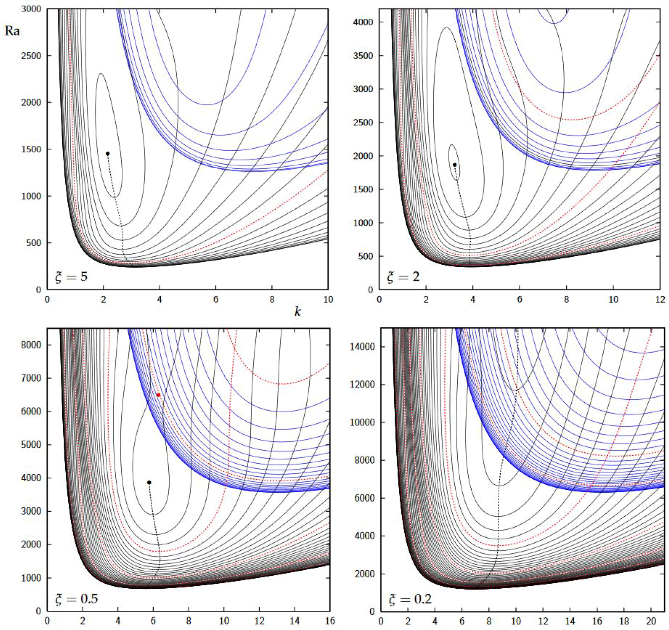
4. Linear Stability Analysis for Three-Dimensional Disturbances

4.1. Reduction to ODE Eigenvalue Form

The linear stability characteristics of the basic steady state to generally oblique roll disturbances may be investigated by setting,
p = p b + p 1 , θ = θ b + θ 1 ,
where p 1 and θ 1 are asymptotically small perturbations in the pressure and temperature, respectively. The substitution of the expressions (29) into the governing Equations (15) and (16) gives the following set of linearised perturbation equations
ξ 2 p 1 x 2 + 2 p 1 y 2 + 2 p 1 z 2 = Ra ξ θ 1 x sin α + θ 1 y cos α ,
θ 1 t + Ra θ b ξ θ 1 x sin α + θ 1 y cos α + Ra θ 1 θ b y cos α ξ p b x θ 1 x + p b y θ 1 y + p 1 y θ b y = 2 θ 1
We Fourier-decompose the perturbations in the x- and z-directions by setting
p 1 θ 1 = P ( y ) Θ ( y ) exp [ i k ( x sin ϕ + z cos ϕ ) + λ t ] ,
where ϕ is the orientation of the roll relative to the x-axis, and where k and λ are once more the wave number of the vortex/cell amd the exponential growth rate, respectively. Expressions (32), when substituted into Equations (30) and (31), reduce the perturbation equations to a set of ordinary differential equations for the reduced disturbance amplitudes, P and Θ :
P k 2 ξ sin 2 ϕ + cos 2 ϕ P = Ra i k ξ Θ sin ϕ sin α + Θ cos α ,
Θ k 2 Θ = 1 2 Ra ( y 2 + y 1 6 ) i k ξ Θ sin ϕ sin α + 1 2 Ra ( 1 2 y ) Θ cos α 1 2 ( 1 2 y ) P + λ Θ .
The boundary conditions are,
P ( 0 ) = Θ ( 0 ) = 0 , P ( 1 ) = Θ ( 1 ) = 0 .

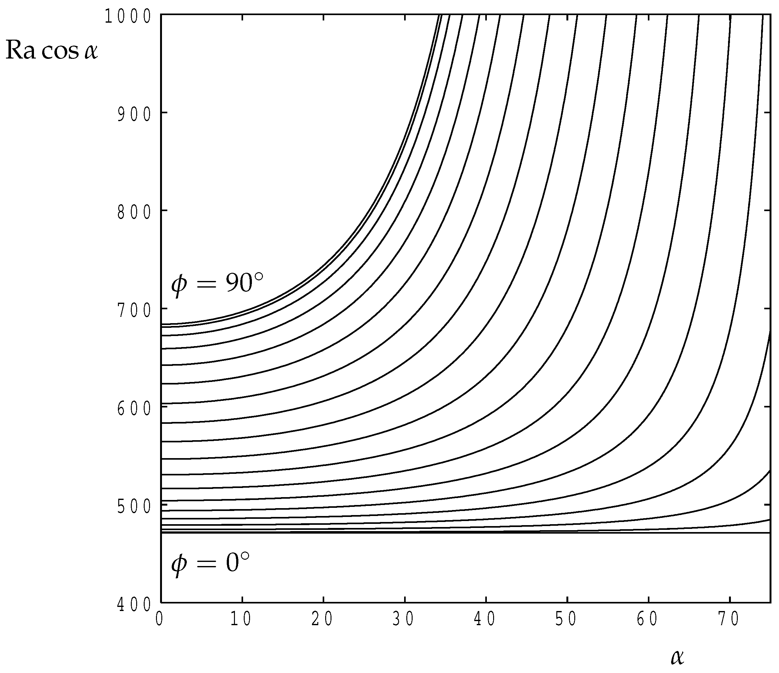
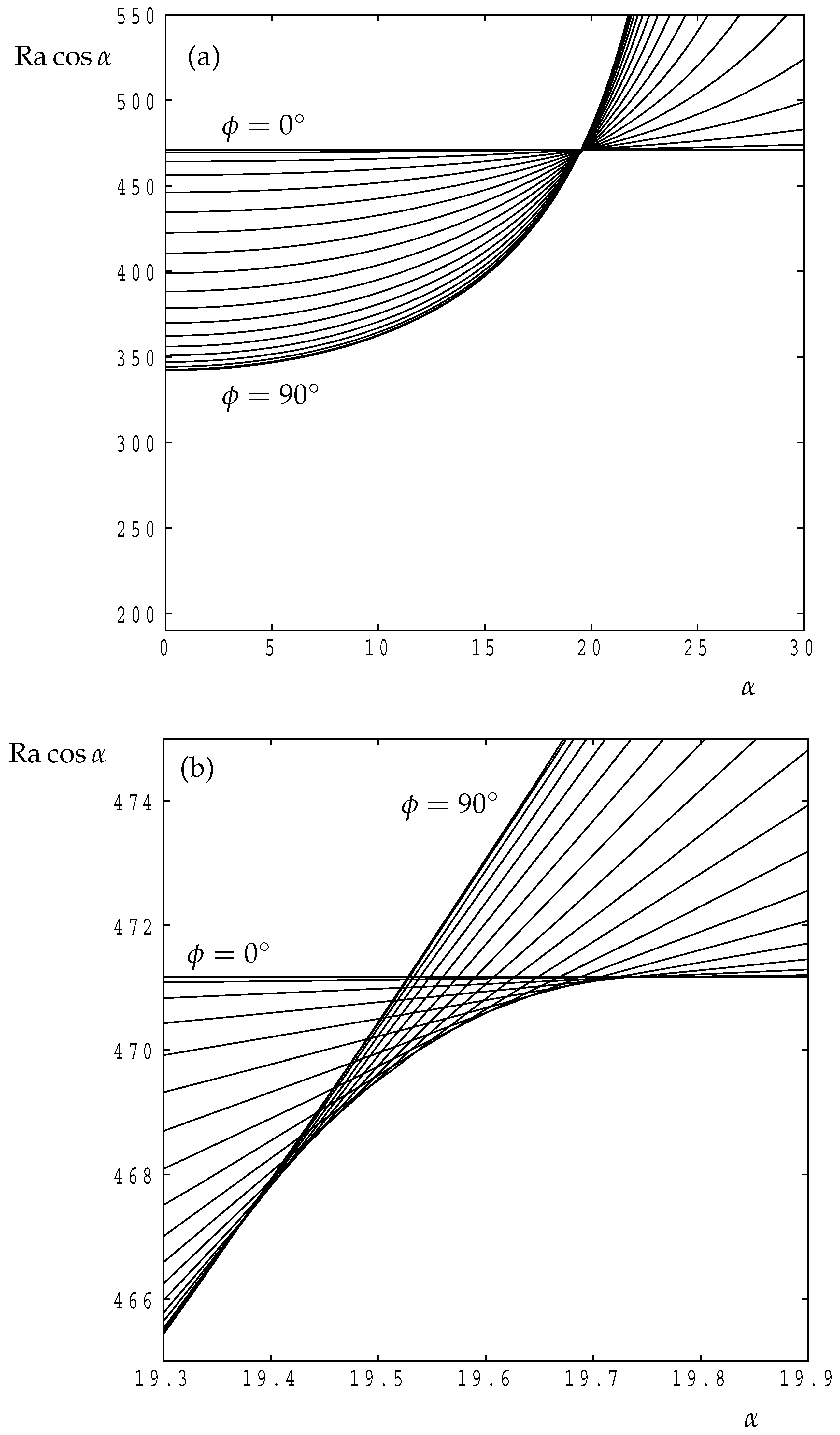
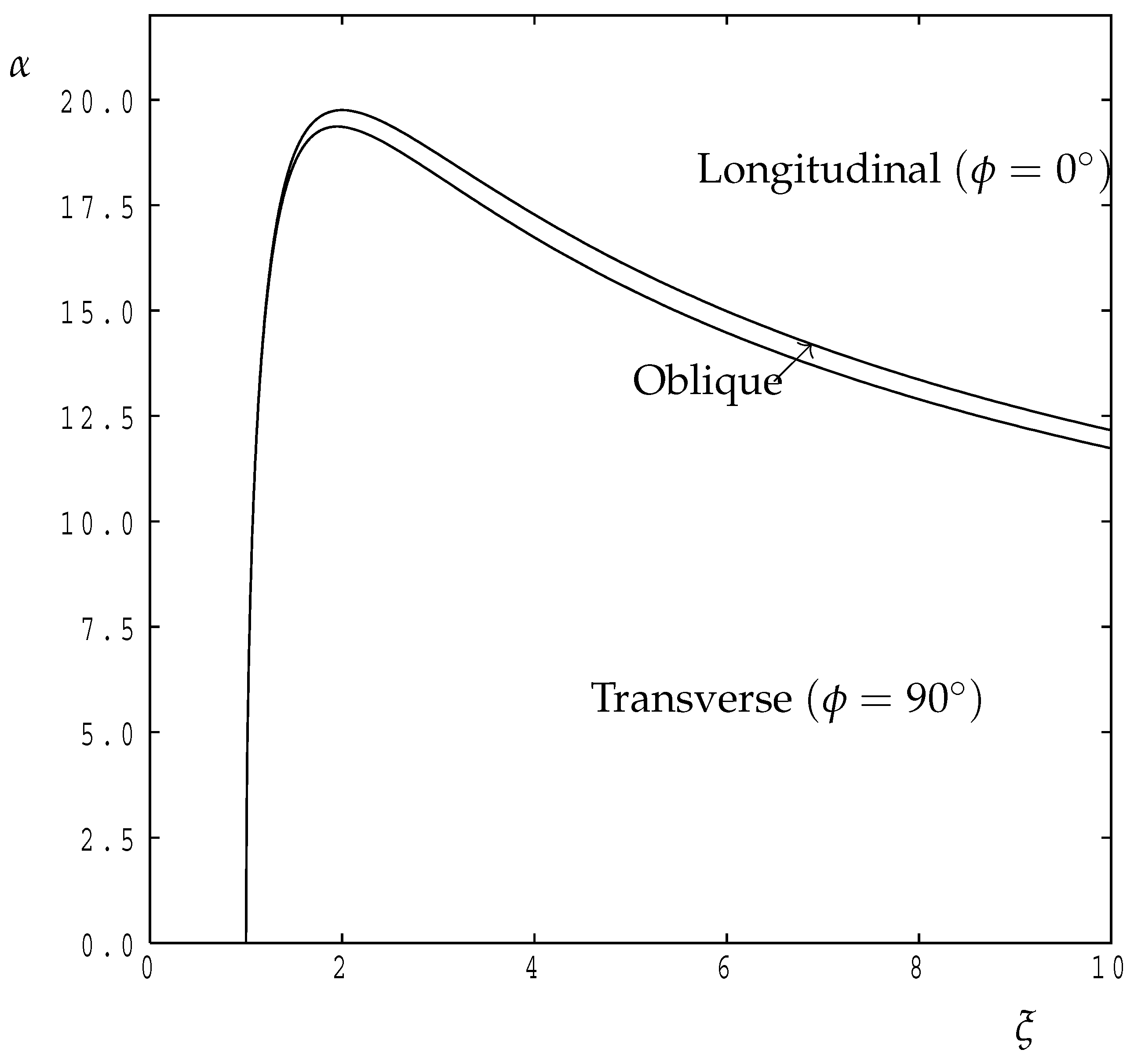
4.2. Numerical Results

Equations (33) and (34) subject to boundary conditions (35) were solved using precisely the same methodology as was used in [27,29], which is a variant of the well-known Keller box method. First, Equation (33) was differentiated once to obtain a second order equation in P so that the boundary conditions for both variables, P and Θ are Dirichlet and thereby absolute accuracy is increased. Second, the resulting equations are supplemented by a system obtained by differentiating these equations with respect to k where Ra / k = 0 is insisted upon in order to minimise the critical Rayleigh number with respect to the wavenumber. Finally the full system was discretised using second order accurate central differences and solved using the modified Keller box method which is described in [27]. This method allows for the computation of eigenvalues which, in this case, are Ra c , k c , λ i and λ i / k . The usual block tridiagonal structure of the iteration matrix is replaced by with an addition row and column of blocks because of the presence of the eigenvalues. A curve-following methodology was also implemented which allows the neutral curve to be followed in Ra - α space for each chosen value of ξ and ϕ . Thus a fifth ‘eigenvalue’ is required which measures the length of the curve being followed. The code used for this work was cross-calibrated by solving the same equations using a standard fourth order Runge-Kutta scheme embedded in a boundary value problem solver.
Figure 7 displays the variation of the critical value of Ra c cos α with α for a range of roll orientations for ξ = 0.5 . For these three-dimensional cases we have chosen to use Ra c cos α rather than Ra c in order to visualize more easily the behaviour of the system and also to avoid Ra c tending towards infinity as the layer tends towards being vertical. In particular we obtain that Ra c = 471.17 / cos α with k c = 4.675 . The message which arises from Figure 7 is that longitudinal rolls are preferred over all other orientations when ξ < 1 , a general result which accords with the analysis of [27]. In these circumstances there is more resistance to flow in the longitudinal or x-direction than in the other two directions, and it is natural therefore to expect the favoured rolls to have axes in the x-direction.
When ξ > 1 the situation becomes more complicated. At small inclinations, i.e., when α is small, then transverse rolls ( ϕ = 90 ) form the preferred orientation, but longitudinal rolls are preferred at much higher inclinations. In the inclined Darcy-Bénard problem studied by Storesletten and Tveitereid [32] it was found that there exists a critical inclination below which transverse rolls are preferred and above which longitudinal rolls are preferred. In the more general problem studied by Rees and Postelnicu [27] the transition was found not to be sudden, but, when ξ takes values which are not too large, there exists a smooth transition where the preferred roll orientation varies continuously between ϕ = 90 and ϕ = 0 as α increases. It is this latter behaviour which we have found to occur in the present problem.
In Figure 8 and Figure 9 we display the variation of Ra cos α with α for a range of values of ϕ ( 0 , 5 , 10 , ⋯, 90 ) for ξ = 2 and 5, respectively. In Figure 8 we see that the transition between transverse rolls at lower inclinations and longitudinal rolls at higher inclinations takes place close to α = 19.6 . This transition is smooth, as shown in the second frame of Figure 8, and it takes place very rapidly over an inclination range of roughly 0.4 .
Figure 9 shows the general behaviour of the neutral curves for the more anisotropic case, ξ = 5 . Again there exists a smooth transition between transverse and longitudinal rolls, but it now extends over a slightly larger inclination range of 0.54 and is centred at roughly α = 15.75 .
In both the cases considered above and for general values of ξ , it is possible to minimise the value of Ra c cos α with respect to ϕ in order to determine the overall minimum critical Rayleigh number as a function of both the inclination and the anisotropy parameter. The results of this process are displayed in Figure 10 which shows how the critical Rayleigh number, and the corresponding roll orientations and wavenumbers vary, and we have selected six different values of ξ > 1 to illustrate the general behaviour. The curves for ξ = 2 and 5 follow the lower envelope of those shown in Figure 8 and Figure 9, respectively.
It is clear that the transition from transverse rolls ( ϕ = 90 ) to longitudinal rolls ( ϕ = 0 ) increases from α = 0 initially as ξ increases from 1 upwards. When ξ is close to 2 this increase in the transition inclination reverses direction and begins to decrease once more as ξ increases further. The rapid variation in the transition process is captured well in the frames displaying k c and the roll orientation, ϕ .
Finally, it is of interest to determine an overall summary of the properties of the present layer in terms of the identity of the convection pattern which is to be expected in practice. This is given in Figure 11, which displays the regions in ( α / ξ ) -space wherein longitudinal, oblique or transverse rolls form the preferred pattern at onset. The rapid transition between transverse and longitudinal rolls as α increases is now very evident due to the closeness of the two curves, and the above-mentioned maximum inclination angle corresponding to ξ 2 is also clear. The curves become extremely close when ξ 1 + and our numerical data suggests that,
α ( ξ 1 ) 1 / 2 41.15 48.2 ( ξ 1 ) ϕ = 0 , 41.15 49.2 ( ξ 1 ) ϕ = 90 .
Therefore the transition range between these extreme orientations is roughly ( ξ 1 ) 3 / 2 as ξ 1 . On the other hand, when ξ takes values which are larger than those shown in Figure 11 then the inclinations at which transitions happen continue to decrease. Some more extreme examples are given in Table 1. These values were obtained by insisting that 2 Ra c / ϕ 2 = 0 , and from this data it is possible to shown (using some error analysis and Richardson extrapolation) that the transition zone (i.e., the range of values of α for which oblique rolls are preferred) occupies the range,
39.85 ξ 1 / 2 α 41.15 ξ 1 / 2 .
when ξ 1 .

5. Conclusions

The onset of convection has been considered for a porous layer which is inclined to the horizontal, is anisotropic and is subject to a uniform internal heat generation. When the Rayleigh number is sufficiently large, instability occurs, and a convective motion is set up. The critical Rayleigh number at the onset of convection then depends very strongly on the anisotropy ratio as well as the inclination angle. Indeed the preferred orientation of convection rolls at onset can depend quite strongly on these parameters.
We have shown that, when ξ < 1 then convection rolls are longitudinal (i.e., with axes in the x-direction) for all inclinations. Numerically we found that Ra c cos α = 471.17 and critical wavenumber k c = 4.675 . However, when the flow is confined to being two dimensional, it has been shown that convection happens for only a finite range of inclinations which is dependent on the anisotropy parameter, ξ . Moreover, when ξ > 0.27843 the neutral curves display an isola point meaning that there a local maximum inclination above which the basic flow is linearly stable.
When ξ > 1 the general situation is more complicated. At small inclinations transverse rolls ( ϕ = 90 ) form the preferred orientation, but longitudinal rolls ( ϕ = 0 ) are preferred at much higher inclinations. In general, the critical Rayleigh number increases as the inclination of the layer increases, but the identity of the favoured roll orientation changes from transverse to longitudinal. The transition between these extreme orientations takes place smoothly but rather rapidly as the inclination, α , increases. The associated variation in the critical wavenumbers becomes more extreme as the anisotropy ratio ξ increases. We have also ascertained that the narrow transition region is centred on values of α which are close to zero both as ξ 1 + and as ξ , and that transition region itself tends towards a zero width for each of those limits.

Author Contributions

Computations: D.A.S.R. Otherwise both authors contributed equally to all aspects.

Funding

This research received no external funding.

Conflicts of Interest

The authors declare no conflict of interest.

Abbreviations

cphase velocity
ggravitational acceleration
hthickness of layer
kwavenumber
K L longitudinal permeability
K T transverse permeability
ppressure
qrate of heat generation
RaDarcy-Rayleigh number
Tdimensional temperature
uvelocity in the x-direction
vvelocity in the y-direction
wvelocity in the z-direction
xcoordinate up the layer
ycoordinate across the layer
zspanwise coordinate
Greek symbols
α inclination angle
β coefficient of thermal expansion
θ nondimensional temperature
κ thermal diffusivity
λ growth rate
μ dynamic viscosity
ξ anisotropy ratio
ρ density
σ heat capacity ratio
ϕ orientation of roll
ψ streamfunction
Subscripts, superscripts, and other symbols
*dimensional
differentiation with respect to y
_amplitude
0reference quantity
1perturbation
bsteady basic flow
ccritical value

References

  1. Horton, C.W.; Rogers, F.T. Convection currents in a porous medium. J. Appl. Phys. 1945, 16, 367–370. [Google Scholar] [CrossRef]
  2. Lapwood, E.R. Convection of a fluid in a porous medium. Proc. Camb. Philos. Soc. 1948, 44, 508–521. [Google Scholar] [CrossRef]
  3. Kulacki, F.A.; Ramchandani, R. Hydrodynamic instability in porous layer saturated with heat-generating fluid. Wärme-Stoffübertrag 1975, 8, 179–185. [Google Scholar] [CrossRef]
  4. Gasser, R.D.; Kazimi, M.S. Onset of convection in a porous medium with internal heat generation. ASME J. Heat Transf. 1976, 98, 49–54. [Google Scholar] [CrossRef]
  5. Buretta, R.J.; Berman, A.S. Convective heat transfer in a liquid saturated porous layer. ASME J. Appl. Mech. 1976, 43, 249–253. [Google Scholar] [CrossRef]
  6. Hardee, H.C.; Nilson, R.H. Natural convection in porous media with heat generation. Nucl. Sci. Eng. 1977, 63, 119–132. [Google Scholar] [CrossRef]
  7. Hwang, I.T.; Marr, W.W. Onset of thermal-convection in a fluid-saturated porous layer with heat source. Trans. Am. Nuclear Soc. 1977, 27, 655–656. [Google Scholar]
  8. Tveitereid, M. Thermal convection in a horizontal porous layer with internal heat sources. Int. J. Heat Mass Transf. 1977, 20, 1045–1050. [Google Scholar] [CrossRef]
  9. Rhee, S.J.; Dhir, V.K.; Catton, I. Natural convection heat transfer in beds of inductively heated particles. ASME J. Heat Transf. 1978, 100, 78–85. [Google Scholar] [CrossRef]
  10. Kulacki, F.A.; Freeman, R.G. A note on thermal convection in a saturated, heat generating porous layer. ASME J. Heat Transf. 1979, 101, 169–171. [Google Scholar] [CrossRef]
  11. Barletta, A.; Celli, M.; Nield, D.A. Unstable buoyant flow in an inclined porous layer with an internal heat source. Int. J. Therm. Sci. 2014, 79, 176–182. [Google Scholar] [CrossRef]
  12. Nandal, R.; Mahajan, A. Linear and nonlinear stability analysis of a Horton-Rogers-Lapwood problem with an internal heat sources and Brinkman effects. Transp. Porous Media 2017, 117, 261–280. [Google Scholar] [CrossRef]
  13. Nouri-Borujerdi, A.; Noghrehabadi, A.R.; Rees, D.A.S. Influence of Darcy number on the onset of convection in a porous layer with a uniform heat source. Int. J. Therm. Sci. 2008, 47, 1020–1025. [Google Scholar] [CrossRef]
  14. Nouri-Borujerdi, A.; Noghrehabadi, A.R.; Rees, D.A.S. The onset of convection in a horizontal porous layer with uniform heat generation using a thermal non-equilibrium model. Transp. Porous Media 2007, 69, 343–357. [Google Scholar] [CrossRef]
  15. Nield, D.A.; Kuznetsov, A.V. The onset of convection in a horizontal porous layer with spatially non-uniform internal heating. Transp. Porous Media 2016, 111, 541–553. [Google Scholar] [CrossRef]
  16. Nield, D.A.; Kuznetsov, A.V. Onset of convection in with internal heating in a weakly heterogeneous porous medium. Transp. Porous Media 2013, 98, 543–552. [Google Scholar] [CrossRef]
  17. Kuznetsov, A.V.; Nield, D.A. The effect of strong heterogeneity on the onset of convection induced by internal heating in a porous medium: A layered model. Transp. Porous Media 2013, 99, 85–100. [Google Scholar] [CrossRef]
  18. Matta, A.; Hill, A.A. Double-diffusive convection in an inclined porous layer with a concentration-based internal heat source. Contin. Mech. Thermodyn. 2018, 30, 165–173. [Google Scholar] [CrossRef]
  19. Mahajan, A.; Nandal, R. Stability of an anisotropic porous layer with internal heat source and Brinkman effects. Spec. Top. Rev. Porous Media 2019, 10, 65–87. [Google Scholar] [CrossRef]
  20. Yadav, D.; Wang, J.; Lee, J. Onset of Darcy-Brinkman convection in a rotating porous layer induced by purely internal heating. J. Porous Media 2017, 20, 691–706. [Google Scholar] [CrossRef]
  21. Malashetty, M.S.; Swamy, M.S. The onset of convection in a viscoelastic liquid saturated anisotropic porous layer. Transp. Porous Media 2007, 67, 203–218. [Google Scholar] [CrossRef]
  22. Yovogan, J.; Miwadinou, C.H.; Claude, E.V.; Degan, G. Effect of anisotropy in permeability on thermal convection of viscoelastic fluids in rotating porous layer heated from below. Aust. J. Mech. Eng. 2018. [Google Scholar] [CrossRef]
  23. Raghunatha, K.R.; Shivakumara, I.S.; Sowbhagya, A.A. Stability of buoyancy-driven convection in an Oldroyd-B fluid-saturated anisotropic porous layer. Appl. Math. Mech. 2018, 39, 653–666. [Google Scholar] [CrossRef]
  24. Abdelhafez, M.A.; Tsybulin, V.G. Modeling of anisotropic convection for the binary fluid in porous medium. Comput. Res. Model. 2018, 10, 801–816. [Google Scholar] [CrossRef]
  25. Yadav, D.; Kim, M.C. Theoretical and numerical analyses on the onset and growth of convective instabilities in a horizontal anisotropic porous medium. J. Porous Media 2014, 17, 1061–1074. [Google Scholar] [CrossRef]
  26. Rees, D.A.S.; Storesletten, L. The linear instability of a thermal boundary layer with suction in an anisotropic porous medium. Fluid Dyn. Res. 2002, 30, 155–168. [Google Scholar] [CrossRef]
  27. Rees, D.A.S.; Postelnicu, A. The onset of convection in an inclined anisotropic porous layer. Int. J. Heat Mass Transf. 2001, 44, 4127–4138. [Google Scholar] [CrossRef]
  28. Postelnicu, A.; Rees, D.A.S. The onset of convection in an anisotropic porous layer inclined at a small angle from the horizontal. Int. Commun. Heat Mass Transf. 2001, 28, 641–650. [Google Scholar] [CrossRef]
  29. Rees, D.A.S.; Storesletten, L.; Postelnicu, A. The onset of convection in an inclined anisotropic porous layer with oblique principle axes. Transp. Porous Media 2006, 62, 139–156. [Google Scholar] [CrossRef]
  30. Capone, F.; Gentile, M.; Hill, A.A. Penetrative convection via internal heating in anisotropic porous media. Mech. Res. Commun. 2010, 37, 441–444. [Google Scholar] [CrossRef]
  31. Rees, D.A.S.; Bassom, A.P. Onset of Darcy-Bénard convection in an inclined porous layer heated from below. Acta Mech. 2000, 144, 103–118. [Google Scholar] [CrossRef]
  32. Storesletten, L.; Tveitereid, M. Onset of convection in an inclined porous layer with anisotropic permeability. Appl. Mech. Eng. 1999, 4, 575–587. [Google Scholar]
Figure 1. Definition sketch of the inclined layer showing the coordinate directions, the inclination angle, α , and the direction of the rolls, ϕ , relative to the x-direction. (a) side view; (b) plan view.
Fluids 04 00075 g001
Figure 2. Showing neutral curves for transverse rolls for ξ = 5 , ξ = 2 , ξ = 0.5 and ξ = 0.2 , and for different inclinations, α , from 0 onwards in increments of 1 . Black curves correspond to mode 1 and blue curves to mode 2. Red dotted curves correspond to α being a multiple of 10 . The black dotted line is the locus of minima while the black disk corresponds to the isola point, i.e., the largest inclination for which there is marginal stability. The red disk corresponds to a saddle point.
Fluids 04 00075 g002
Figure 3. Showing the variation of Ra c for transverse roll disturbances at critical points on the neutral curve for ξ = 0.2 (far right), 0.3 , 0.4 , 0.5 , 0.7 , 1, 2, 3, 5 and 10 (far left). The black disks correspond either to isola points or to saddle points. The dotted lines correspond to isolae (lower curve) and saddle points (upper curve) in the surface, α = α ( Ra , k ) .
Fluids 04 00075 g003
Figure 4. Showing the variation of k c for transverse roll disturbances at critical points on the neutral curve for ξ = 0.2 (uppermost), 0.3 , 0.4 , 0.5 , 0.7 , 1, 2, 3, 5 and 10 (lowest). The black disks correspond either to isola points or to saddle points.
Fluids 04 00075 g004
Figure 5. Showing the variation of c, the phase velocity of transverse roll disturbances, at critical points on the neutral curve for ξ = 0.2 , 0.3 , 0.4 , 0.5 , 0.7 , 1, 2, 3, 5 and 10. The black disks correspond either to isola points or to saddle points.
Fluids 04 00075 g005
Figure 6. Showing the disturbance isotherms for one spatial period for transverse rolls when ξ = 5 . The isotherms are at 20 equally-spaced intervals in each case.
Fluids 04 00075 g006
Figure 7. For ξ = 0.5 . The variation with α of the critical value of Ra cos α for the roll orientations, ϕ = 0 , 5 , 10 , …, 90 .
Fluids 04 00075 g007
Figure 8. For ξ = 2 . (a) the variation with α of the critical value of Ra cos α for the roll orientations, ϕ = 0 , 5 , 10 , …, 90 . (b) Showing a close-up view of the smooth transition between transverse and longitudinal rolls.
Fluids 04 00075 g008
Figure 9. For ξ = 5 . (a) the variation with α of the critical value of Ra cos α for the roll orientations, ϕ = 0 , 5 , 10 , …, 90 . (b) Showing a close-up view of the smooth transition between transverse and longitudinal rolls.
Fluids 04 00075 g009
Figure 10. As functions of the inclination, α : (a) the critical value of Ra cos α which has been minimised over both wavenuber and roll orientation; (b) the corresponding wavenumber; (c) the corresponding roll orientation in degrees. For ξ = 1 , 1.1 , 1.5 and 2 (continuous lines) and for ξ = 3 , 5 and 10 (dotted lines).
Fluids 04 00075 g010
Figure 11. Showing the different regions in ( ξ , α ) –space wherein longitudinal rolls, oblique rolls (between the two curves) and transverse rolls form the most unstable planform of convection.
Fluids 04 00075 g011
Table 1. Transitional values of α when ξ is large; see Figure 11.
ξ for ϕ = 90 for ϕ = 0
125 3.542304 3.660913
250 2.512439 2.595616
500 1.779291 1.837828
1000 1.259118 1.300388

