1. Introduction
In coastal areas, steep bathymetries and strong currents are often observed. Among several causes, the presence of cliffs, rocky beds, or human structures may cause strong variations of the sea bed, while oceanic circulation, tides, wind action, or wave breaking can be responsible for the generation of strong currents. For both coastal safety and engineering purposes, there is strong interest in providing efficient models predicting the nonlinear, phase-resolved behavior of water waves in such areas. This leads to computational difficulties, since large computational areas often need to be considered, and the evolution of water waves propagating in such inhomogeneous media involves multiple-scale phenomena. Moreover, many physical processes influence the dynamics of water waves in such cases, due to reflection, refraction, and diffraction of water waves, in conjunction with nonlinear wave–bottom, wave–current, and wave–vorticity interactions, and the description of these processes requires careful attention.
Various attempts to partially treat the above problems are found in the literature. Starting with depth-averaged models, the mild-slope equation [
1,
2] was derived to describe refraction, diffraction, and reflection of dispersive water waves over varying bathymetry. The derivation is based on the assumption that the vertical structure of the wave field is represented by hyperbolic cosine function, and thus, the mild-slope equation is restrained to the description of linear water waves evolving on slowly varying bathymetries with respect to the wavelength. Similarly, Boussinesq models [
1,
3] have been derived by using a polynomial function. Later, Massel [
4] and Chamberlain and Porter [
5] provided an extension of mild-slope models by considering higher order approximations with respect to the bed-slope parameter. Furthermore, Massel [
4] suggested a multi-modal expansion to improve the representation of the vertical distribution of the wave field deriving a set of coupled equations, involving both propagating and evanescent modes. The latter approach has been further improved by Athanassoulis and Belibassakis [
6] by including extra terms to consistently treat the boundary conditions. This approach has been extended to nonlinear equations [
7,
8], and many solvers are now based on similar techniques, e.g., Raoult et al. [
9]. The above techniques have demonstrated their efficiency in modeling wave–bottom interactions in inhomogeneous environments. Similar developments for modelling wave–current interactions have been presented by various authors, e.g., Booij [
10], Liu [
11], and Kirby [
12]. The current considered in the above works is assumed to be slowly varying in horizontal directions and uniform in depth. In the same direction, coupled-mode models have also been derived [
13].
More recently, it was established that the vorticity involved in vertically non-uniform currents could have significant effects on the propagation of water waves [
14]. This gave rise to new derivations of models aiming to describe this interaction. In the case of currents with locally constant shear, extended mild slope models, similar to those derived by Berkhoff and Kirby, have been obtained [
15,
16], and at the next stage, a coupled mode model was derived [
17]. The importance of this approach was recently validated experimentally in a previous study [
18]. In these works, the currents were assumed to vary linearly with depth. If this case is realistic in some specific configurations [
19,
20], it might be suggested that when the current contains strong vorticity it will have more complicated vertical distribution. In the case when the second vertical derivative of the mean current flow is zero, the vorticity conservation equation for water waves involves no source term [
20]. Furthermore, in the case of mild horizontal variations of the shear, its effect can be approximately neglected, and water waves can be approximately described as irrotational [
18].
The present work aims to extend the validity of the above models to more general current configurations. Indeed, if the vorticity conservation equation involves a source term, due to the interaction of the flow with the sheared current, water waves cannot be treated as irrotational anymore. For this purpose, the present novel coupled-mode system is obtained in the framework of Euler equations by using a velocity-based formulation, allowing one to describe wave–vorticity interactions in more generic conditions.
The present paper is structured as follows. After the introduction, the modal expansion of the velocity field is introduced in
Section 2 using a Fourier-type basis generated by local vertical eigenproblems. In particular, the present formulation is based on a velocity representation defined by a series of local vertical modes containing the propagating and evanescent modes, able to accurately treat the continuity condition and the bottom boundary condition on sloping parts of the seabed. Using the above representation in Euler equations, in
Section 3 a coupled system of differential equations on the horizontal plane is derived, with respect to the unknown horizontal velocity modal amplitudes. Subsequently,
Section 5 is dedicated to the analysis of the dispersive behavior of this system under linearity assumptions, and finally, numerical examples are presented and discussed in
Section 6 in order to illustrate the ability of the present system to reproduce classical propagation configurations. Finally, the main conclusions are presented, including directions for further research.
2. Vertical Expansion of the Velocity Field
In the present work we will restrict ourselves to 2D problems corresponding to waves propagating in a vertical strip under the additional effects by collinear currents. However, the present analysis can be extended in two horizontal dimensions, and this is left to be considered along with 3D applications in future work.
Let
denote the flow domain bounded below by the bottom boundary defined by the depth function,
, and above by the free-surface defined by the corresponding elevation,
; see
Figure 1. We assume that
. In this work, we exploit a local-mode series expansion of the wave velocity
in variable bathymetry regions. It is based on extension of similar developed models, under the assumption of irrotationality, for the wave potential by Athanassoulis and Belibassakis [
6] for the linearized problem and subsequently for non-linear wave problems [
7,
8]. This expansion has the general form of summation of local modes (each one numbered by an integer index). In particular, the local-mode representation of the horizontal velocity component reads as follows:
where
denote vertical functions that are parametrically dependent on the bathymetry and the free-surface elevation, having the properties to satisfy the continuity equation, the bottom boundary condition, and to be complete in local vertical intervals
. More specifically, the functions
are defined as follows
where the quantities
are obtained as the roots of the (dispersion-like) equations
The first root is imaginary
and the rest
are real, with
. The completeness property of the vertical basis stems from the fact that
are generated from regular vertical Sturm-Liouville eigenproblems in the local vertical
, controlled by the frequency-type parameter
; see also Belibassakis and Athanassoulis [
8]. The latter parameter (or in non-dimensional form
, with
denoting a characteristic depth) is not subjected to a priori restrictions. However, the specific values of these parameters influence the accuracy of truncated versions of the local-mode series, as will be illustrated in the sequel concerning the convergence of the expansion and the dispersion characteristics of the present model.
The vertical component
of the velocity field is represented by a corresponding modal series based on a new set of vertical functions
, as follows
and thus, it is expressed as follows
where the new vertical functions
are defined to automatically satisfy the wave kinematics, which are defined by continuity condition in the water column
and the bottom boundary condition
It is easily verified that the above constraints are fulfilled by selecting the functions
to satisfy the requirement
leading to the following analytic expression of the new set of vertical functions
In fact, from Equations (5) and (9) we see that the bottom vertical velocity is given by
The latter used in the bottom boundary condition, Equation (6), it finally leads to
since, from Equation (8), it is obtained that
. Details concerning the latter results are provided in
Appendix A.
Moreover, the continuity condition, for all
x, and
, is identically satisfied
The usefulness of the above local-mode representations, Equations (1) and (5), is that used in the momentum equations will lead to a non-linear coupled-mode system of differential equations on the horizontal plane, with respect to unknown modal amplitudes
and the unknown free-surface elevation
. The coupled-mode system, in conjunction with the fast convergence properties of the local mode series, greatly facilitates the numerical solution of the present problem and will be presented in the next section. Similar modal-type series expansion has been previously introduced by Nadaoka et al. [
21] for the development of a fully dispersive, weakly nonlinear, multiterm-coupling model for water waves, with application to slowly varying bottom topography. In that work, the vertical modes have been selected to have the form
, where the parameters
are independent from the free surface elevation
. This approach can be considered as an extension of Fourier methods above a flat bottom [
22,
23] to variable bathymetry regions characterized by a mildly sloped bottom.
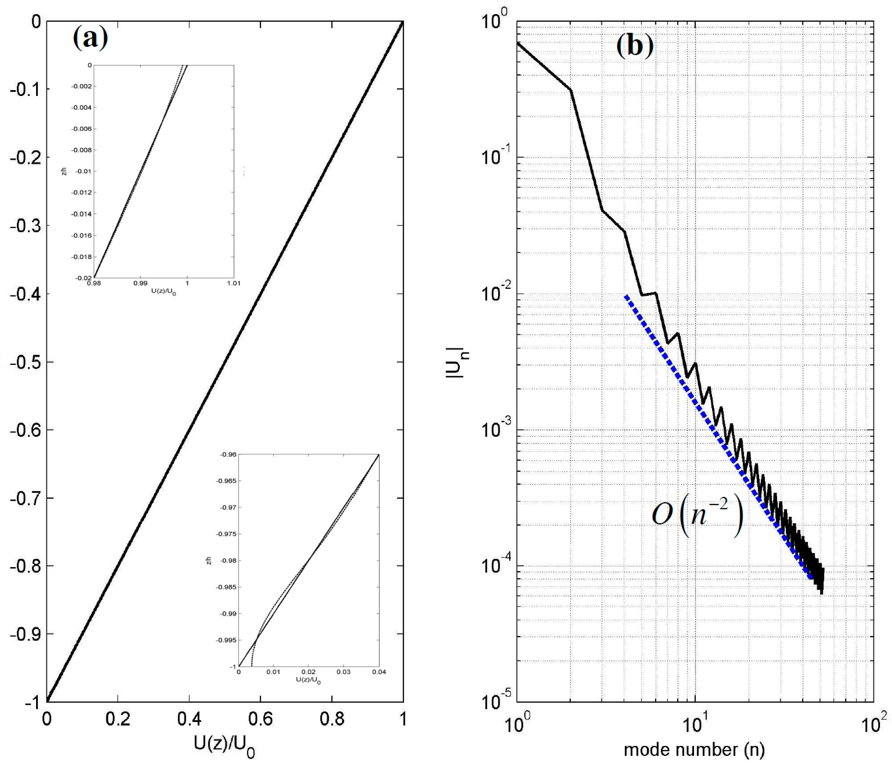
As it is presented and discussed in more detail in
Appendix B, the expected rate of convergence of the modal series (1) is
, where
n is the mode number. Under the assumption of smooth upper
and lower
boundaries, the above rate ensures that
. The latter is sufficient for the solution of the wave flow problem by a spectral Galerkin-type method that will be presented in the next section, as obtained by projecting the momentum flow equations on the vertical basis
, for each instant and at each horizontal
x-position.
The modal representation Equation (1) can be further improved by introducing additional modes in the series expansion, as presented by Athanassoulis and Belibassakis [
6,
7] for the wave potential [
24]. In the latter works the additional slopping-bottom and free-surface modes treat the inconsistency between the boundary conditions of the potential at
, and the boundary conditions satisfied by the Sturm-Liouville problem generating the vertical basis. This accelerates the convergence of the modal series by increasing the rate of decay of the potential amplitudes from
to
. In the present case, there is also an inconsistency for the velocity field
but only at the free surface
, and could be similarly treated accelerating the convergence. However, it should be mentioned that application of the present model to the special case of irrotational flows, without any additional modes for the expansions of
and
, leads to a decay rate
, which would correspond to
concerning the underlying potential modes, as obtained by direct integration.
Two examples illustrating the above results in the case of irrotational wave-like field under a sinusoidal upper surface of large amplitude and a vertically sheared Couette flow between horizontal planes are presented and discussed in
Appendix B.
3. Momentum Equations
In the previous section it is shown that through the appropriate selection of vertical expansions of the velocity field, the kinematics of the wave problem concerning continuity and bottom surface boundary condition are analytically satisfied. Thus, we are left with the requirement of the momentum equations and the free surface boundary conditions, including the kinematic and the dynamic ones.
Neglecting the effect of viscous dissipation in the fluid volume, the momentum equations in the horizontal and vertical components are, respectively,
where
and
, an helicity-type field, with
denoting the vorticity
, which in the present two-dimensional case is fixed in the transverse direction (with
denoting the corresponding unit vector). Thus, in the present 1DH case,
Subsequently, we may consider at each horizontal
x-position, the vertical momentum Equation (13) integrated in the vertical direction from a depth level z up to the free surface elevation
, from which an expression for the pressure in the local column is obtained
Employing in Equation (15) the dynamic free–surface boundary condition
we obtain
The above equation is then differentiated with respect to the horizontal coordinate to obtain
which substituted back to Equation (13) finally results in
for all
and
, where
. The last Equation (19a), in conjunction with the kinematic free-surface boundary condition,
constitute the remaining system to be solved. In the next section, Equations (19a) and (19b) in conjunction with the representations defined by Equations (1) and (4) will be put in the form of a coupled-mode system with respect to the wave velocity modal amplitudes
and the free surface elevation
, constituting the unknown fields in the horizontal domain.
3.1. Irrotational Waves Over Variable Bathymetry
We first consider the case of irrotational waves without a current. In order to reduce it to a coupled system of equations we exploit the completeness properties of the local eigenfunctions
and project both sides of Equation (19a) into the latter vertical basis. Thus, for each horizontal
x-position, we obtain
where
. Furthermore, using the local mode representations defined by Equations (1) and (4), and carrying out the algebra, the following set of equations is derived
where the orthogonality properties of the vertical basis
with
denoting Kronecker’s delta, and
have been also used. Moreover, using the fact that the vertical local eigenfunctions
are normalized by their free surface values (i.e.,
), the kinematic free-surface boundary condition, Equation (19b), takes the following form:
Recalling the fact that the expected rate of decay of modal amplitudes
, specific attention is needed concerning the convergence of the above term-wise differentiated series at
representing the horizontal flow velocity derivatives. In particular, under the assumption that
are expected to decay as
based on evidence that all modes present similar wavelike behavior
which will be illustrated in the examples below, and using the fact that
, which is obtained by straightforward algebra (see also [
24]), the convergence of the series
to the horizontal derivative
is obtained. Furthermore, using the fact that
and thus,
, the series appearing as the last term in Equation (20b) converges to
. Finally, using similar arguments, it can be shown that term-wise differentiation of the latter series converges to
. Substitution of the above modal expansions for
and
in Equation (20), in conjunction with the representations Equations (1) and (4), eventually leads to the present nonlinear coupled-mode system (nCMS) formulated with respect to the horizontal flow velocity amplitudes
and the free surface elevation
as the unknowns. The detailed analysis of the nCMS will be presented in future works.
3.2. Waves and Current Over Bathymetry
In the case of waves propagating under the additional effects of steady currents, the flow variables are split in two components: (i) the wave part
, and (ii) the steady background current
. We furthermore assume that the variation of the current flow is smaller than the corresponding wave flow and that
. Using the above decomposition in Equation (19) and retaining terms to the lowest order [
25], these equations are put in the form
where
denotes differentiation moving with the current.
To reduce to a coupled system of equations, we again exploit the completeness properties of the local eigenfunctions
and project both sides of Equation (21a) into the latter vertical basis. Thus, for each horizontal
x-position, we obtain
where now
. Furthermore, using in Equation (21) the local mode representations defined by Equations (1) and (4), and carrying out the algebra, the following set of equations is derived, assuming also that the vorticity is essentially contained in the current
,
Moreover, using the fact that the vertical local eigenfunctions
are normalized (i.e.,
), the kinematic free-surface boundary condition takes the form:
The above Equations (22) and (23) constitute the present CMS in the case of waves and currents, again formulated with respect to the horizontal flow amplitudes and the free surface elevation as unknowns.
4. Dispersion Characteristics of the Linearized CMS
The set of Equations (22) and (23) is linearized by first dropping the terms involving products of the unknowns. Furthermore, assuming that
, the vertical integrals are restricted up to mean water level
z = 0. In addition, assuming that the vorticity is essentially contained in the current
, we obtain the following expressions of the corresponding terms in Equation (22)
where
, and the functions
,
are obtained from Equations (1) and (4) using
η = 0. Moreover, in the present case
and the brackets denote
. Thus, Equations (22) are put in the following form:
Also, the kinematic free-surface condition, Equation (23), is linearized by dropping the second term and transferring the condition to the level
z = 0
where
and
.
We next consider an environment characterized by constant parameters (constant depth, constant background flow) and use again the local mode representations. Assuming now harmonic time dependence and seeking periodic solutions
in a constant depth strip with range independent steady current
U(
x), we obtain from Equation (24b)
Using the latter result in Equation (24a) we obtain the following homogeneous system
where
, with
the value of the current at the surface. Moreover,
is Kronecker’s delta, and the rest coefficients are given by
For a given wave frequency ω, the periodicity parameter k is found by requiring the determinant of Equation (26) to be zero, which enables us to investigate the dispersion properties of the linearized system and compare against analytical solutions. For this purpose, we truncate the local-mode expansion, Equation (1), keeping a finite number of terms, and investigate the linearized truncated CMS dispersion curve against known analytical solutions.
(i) No current: In the case of waves propagating in constant depth without current (
σ =
ω and
), numerical results obtained as non-trivial solutions of Equation (26) concerning the normalized phase speed
, which depends only on the non-dimensional wavenumber
, are compared against the analytical solution, given by
Results are presented in
Figure 2 for values of the nondimensional wavenumber
from 0 to 2
π, ranging from very shallow to deep wave conditions, and using two values of the parameter controlling the vertical basis:
. A rapid convergence of results to the analytical solution is observed, shown by using thick lines, as the modes included in the present series increases. We also observe in
Figure 2 that the present representation, keeping only the first term (
n = 0) in the expansion, provides excellent results over a bandwidth of non-dimensional wavenumbers around the selected value of the parameter
, indicating that a simplified model based on a single-term approximation of the flow velocity
is able to provide good results with appropriate selection of parameter
.
(ii) Parallel flow: In the case of a uniform current in depth, the flow vorticity is zero (
). Numerical results are obtained as non-trivial solutions of Equation (26) concerning the normalized phase speed
, which now depends both on the frequency parameter
and the bathymetric Froude number
, and compared against the analytical solution
More specifically, for each frequency
ω, the corresponding wavenumber
is derived from the roots of the following dispersion relation
where the case of opposing waves to current correspond to
and following waves to
, respectively.
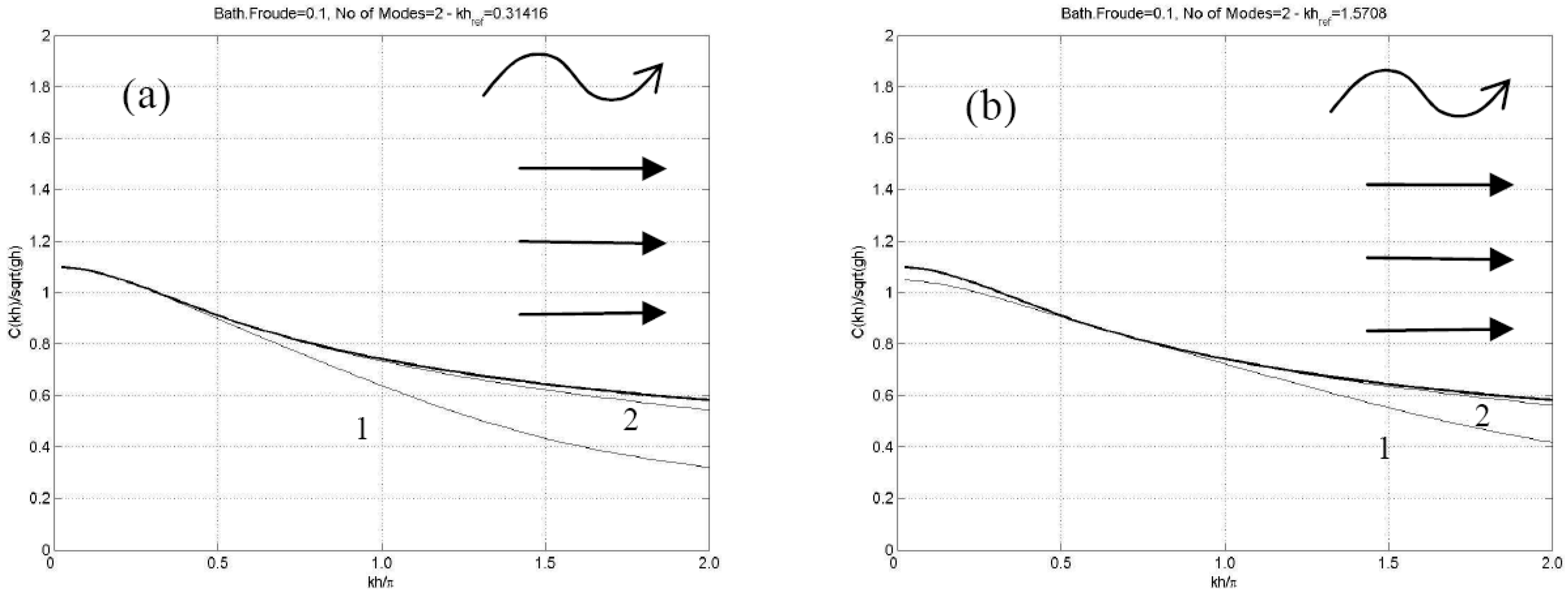
Results concerning a relatively strong current characterized by
= 0.1 for following waves are presented in
Figure 3, again for all values of the non-dimensional wavenumber
, ranging from 0 to 2π, corresponding from very shallow to deep wave conditions. The same as before, two values of the parameter controlling the vertical basis
are used. Again, rapid convergence of present results to the analytical solution, which is shown by using thick lines, is observed as the modes included in the present series increases. The corresponding results in the case of opposing wave and current are presented in
Figure 4. In this case the convergence to the analytical results is slower, especially when the propagation speed becomes smaller approaching the blocking condition. However, in both cases, the present representation, keeping only the first term (
n = 0) in the expansion, provides good results over a bandwidth of non-dimensional wavenumbers around the selected value of the parameter
, rendering the single-term model a good approximation.
(iii) Current with constant vorticity: In the case of a linear vertical profile
, the vorticity is constant in the domain
and the coefficient
in Equation (26) becomes
. Nontrivial solutions of Equation (26) are compared against the dispersion relation. Numerical results obtained as non-trivial solutions of Equation (26) concern the normalized phase speed
. Following a previous study [
16], in this case the dispersion relation is formulated in terms of the frequency parameter
and two bathymetric Froude numbers: one corresponding to the current flow at the surface
and a second one
associated with the current speed at a depth
below the free surface. The latter parameter is also expressed in terms of Froude number
Fh and the nondimensional shear coefficient
, as follows:
.
Again, for each frequency
ω, the corresponding wavenumber
is derived from the roots of the following dispersion relation
and are compared against the analytical solution
Results for following waves and a relatively strong current characterized by
= 0.1 and positive shear
are presented in
Figure 5a,b, while the case of negative shear is presented in
Figure 5c,d. Corresponding results for opposing waves and vertically sheared currents characterized by the same parameters are presented in
Figure 6. The behavior of the present CMS concerning the dispersion is again verified. In all cases the single-term model offers a good approximation for a band of frequencies around the selected value of the parameter
defining the vertical basis. Further investigation of the dispersive properties of the present CMS in cases corresponding to a current with a more general vertical profile and the simulation of waves will be the subject of future work.
5. Numerical Results
In this section, first numerical results concerning the simulation by the present CMS for waves propagating in variable bathymetry regions will be presented. We will first investigate in
Section 5.1 and
Section 5.2 the behavior of the linearized CMS in cases of waves propagating in variable bathymetry regions without and with current effects, respectively, and provide some evidence concerning the convergence of the modal series. This will reveal the characteristics and rate of decay of the modal amplitudes
and will illustrate the significance of the first term
n = 0 in the present modal expansion. Subsequently, the effect of nonlinearity will be demonstrated in
Section 5.3, in the case of wave propagation over bathymetry without current, by using a simplified model based on the truncated local mode series, and keeping only the first
n = 0 term.
5.1. Numerical Solution
The modal series Equations (1) and (4) are truncated, keeping only a finite number of terms, and the present CMS is discretized by using second-order, central finite differences to approximate horizontal and time derivatives of the unknowns and based on a uniform grid , defined by subdividing the horizontal extent of the domain ranging in by using steps of equal length .
Based on the above analysis presented in
Section 4 concerning the dispersion characteristics of the present model, in conjunction with extensive experience from similar applications of the CMS, in most cases the number of the retained modes required for convergence is 4–5, and the horizontal subdivision of the domain is based on using 30–40 points per wavelength. In the examples that will be presented and discussed below, the dimension of the discrete coupled-mode system is of the order of 1500, which is expected to be significantly (orders of magnitude) less than the analysis required for a solution of Euler or Navier-Stokes equations based on a full spatial grid (see Koutrouveli and Dimas [
26]). Moreover, the time interval is
by using constant time steps
. An implicit Crank-Nicolson method for time-integration is considered, satisfying Courant numbers
.
In the examples presented below the depth function changes smoothly from to , such as the bottom slope and curvature are zero at the ends of the domain, the flow motion starts from rest, and boundary conditions are imposed on the wave inlet boundary corresponding to a simple periodic wave corresponding to the depth
. Finally, the reflected back propagating waves in the vicinity of the wave entrance and the radiated waves in the wave exit are absorbed by using a relaxation scheme extending over one characteristic wave length in these regions.
An example concerning harmonic incident waves of period
T = 2 s and a height of 5 cm propagating over a linear upslope with decreasing depth from
= 0.4 m to
= 0.1 m, presenting a bottom slope of 4.5% is presented in
Figure 7. The calculated modes
at a given time instant are plotted along with the velocity field
and the free surface elevation
at the same instant, as obtained by the present linearized CMS, using
. Using the results presented in
Appendix B concerning the rate decay of the mode amplitude, Equations (A4) and (A5), in conjunction with the fact that all modes (
n > 0) follow the phase of the propagating mode (
n = 0) as it can be also observed in
Figure 7, the following trend is expected to be valid:
The latter result has been used in the discussion concerning the convergence of the present modal expansion in
Section 2.
5.2. Wave Propagation Over an Underwater Bar in the Presence of Opposing Shearing Current
As a second example, we consider the case of normal incident waves propagating over a trapezoidal bar, seated on a flat horizontal bottom in the presence of an opposing vertically sheared current, which is presented and discussed in Belibassakis et al. [
17]. In this case, experiments have also been carried out in the wave flume at SeaTech, University of Toulon, France. At the upwave end of the channel, an electromagnetic piston generates regular waves by horizontal motion. Also, at the downwave end, a sloping beach is used to absorb waves. An opposing current is injected in the channel by a hydraulic pump and a perforated screen is used to control the shear. The opposing current is adjusted to generate flow profiles that are linear in depth
, where
is the surface current and
the shear, and thus, in this specific case the vorticity is
. In the experiments, the water depth was 0.305 m, and the incident wave frequencies were ranging from 0.65 Hz to 1.3 Hz with amplitudes between 1–2 cm ensuring small wave steepness, both without and with the vertically sheared current. The distributions of the bathymetry, as well as the surface current and shear data, are presented in
Figure 8.
Furthermore, a coupled–mode model has been developed and discussed in Belibassakis et al. [
17] for the above problem formulated in the frequency domain. The latter model is based on the assumption that the wave field is irrotational, which is a plausible approximation for cases where the current flow and the vorticity structure are simplified and the corresponding parameters are slowly varying horizontal functions. Results from the above coupled mode system have been compared in a previous study [
17] against experimental measurements concerning the reflection coefficient, illustrating that the model is able to provide good predictions.
In order to illustrate the performance of the present system, calculated results are presented in
Figure 9 and
Figure 10 concerning harmonic incident waves of period
T = 1 s and an amplitude of 2 cm propagating over the trapezoidal bar topography, without and with the consideration of the sheared current, using the data of
Figure 8. In particular, in
Figure 9 the calculated modes
at a given time instant are plotted along with the surface wave velocity field
and the free surface elevation
at the same instant, as obtained by the present linearized CMS given by Equation (24), first without the consideration of any current. Again we observe the very fast decay of the mode amplitudes. Moreover, the present solution concerning the free surface elevation calculated at an instant where the wave has reached the absorbing beach is also compared with the time-harmonic solution indicated by using dashed lines, illustrating the compatibility of the present model with previously established ones.
The same behavior is also confirmed in the case of waves propagating against linear vertically sheared current, as shown in
Figure 10, where the corresponding result is presented with the modifications by the presence of the opposing sheared current and compared with the frequency-domain solution. We clearly observe the shortening of the wavelengths due to the effects of the current, and the steepening of waves, especially over the submerged structure.
Moreover, in this case, the disturbance of the flow due to combined effect of variable bathymetry and vorticity contained in the vertically sheared current is seen to generate a more complicated pattern concerning the higher-order modes, especially at the face and rear side of the trapezoidal bar. Further investigation of this behavior, including optimization of the numerical scheme to reduce possible instabilities, with application of the present model to more complex situations and detailed analysis, including comparison against experimental measurements, will be the subject of future work.
5.3. A Single-Mode Weakly Nonlinear Model
Based on the above remarks concerning the convergence of the present modal series, it is useful to consider here a simplified nonlinear model for waves without current effects, derived from Equation (20) by keeping only the
n = 0 term in the expansions of the horizontal
velocity component and dropping the term
as higher-order quantity in the momentum equation. The single-mode, simplified non-linear model reads as follows:
where the coefficients are given by
The linear dispersion characteristics of the above simplified model are the same as the ones of the present CMS with
n = 1 terms shown in
Figure 2. Numerical results in the case of monochromatic waves of period
T = 2 s and a height of 2cm propagating over a trapezoidal bar are shown in
Figure 11 and
Figure 12, as obtained by a simplified version of the present single-mode model defined by Equations (31) and (32), using
. In particular, comparison of the latter model results against the experimental data by Beji and Battjes [
27] concerning a time series of free surface elevation measured at stations 2–7 of
Figure 11 are shown in
Figure 12 by using dotted lines. It is observed that the nonlinear simplified model is able to provide quite good predictions, which is evidence of the good properties of the nonlinear system developed in the present work. Further applications and additional investigation in the case of wave–current interaction over bathymetry will be presented in future work.
6. Conclusions
In this work, a novel coupled-mode system is derived based on a velocity formulation and Euler equations, overcoming the irrotational assumption of standard models of waves propagating in variable bathymetry regions, focusing on the study of additional effects due to inhomogeneous currents. The present work is limited to collinear waves and currents, and the new model is based on a modal expansion of the horizontal component of the velocity field by using a vertical basis defined by local Sturm-Liouville eigenproblems. A corresponding expansion of the vertical velocity component is also derived fulfilling the continuity and the bottom boundary condition. Subsequently, projection of momentum equations in the local vertical basis leads to the new coupled system of equations with respect to the horizontal velocity mode amplitudes and the free-surface elevation, closed by the kinematic free-surface boundary condition.
The dispersive behavior of the present system is analyzed in detail, for: (i) water waves propagating without current, (ii) water waves propagating in the presence of a depth-uniform current (thus involving no vorticity), and (iii) water waves propagating in the presence of a linearly sheared current, thus presenting constant vorticity. In every case, the convergence of the system is rapidly achieved, and good results are obtained by keeping only a few modes in the modal series, for all values of the shallowness parameter ranging from shallow to deep water conditions. First results concerning the numerical performance of the present system are also presented, and a demonstration of the nonlinear behavior of the system is shown through the application of a simplified single-mode model to the case of waves propagating over a trapezoidal bar and comparison against experimental data. After further elaboration, the present system is expected to provide a useful tool for modeling wave–current interactions under the effects of vorticity. Finally, the analytical structure of the present coupled-mode system facilitates extensions to treat non-linear effects and applications concerning 3D wave scattering by inhomogeneous currents in coastal regions with general bottom topography.


