Constructive Study of Modulational Instability in Higher Order Korteweg-de Vries Equations

Abstract

Our present study is devoted to the constructive study of the modulational instability for the Korteweg-de Vries (KdV)-family of equations $u_t+s{u}^p{u}_x+u_{xxx}$ (here $s=\pm 1$ and $p>0$ is an arbitrary integer). For deducing the conditions of the instability, we first computed the nonlinear corrections to the frequency of the Stokes wave and then explored the coefficients of the corresponding modified nonlinear Schrödinger equations, thus deducing explicit expressions for the instability growth rate, maximum of the increment and the boundaries of the instability interval. A brief discussion of the results, open questions and further research directions completes the paper.

1. Introduction

Our present study is devoted to the constructive study of the modulational instability for the class of the generalized Korteweg-de Vries (gKdV) equations of the general form

$$u_t+s{u}^p{u}_x+u_{xxx}=0,s=\pm 1,$$

(1)

where $p>0$ is an arbitrary integer. They describe weakly nonlinear dispersive waves met in various physical problems of fluid mechanics, plasma, astrophysics, oceanography and studied in numerous books and papers, only a few of them can be cited further on. Two fundamental equations of this class with $p=1$ and $p=2$ are well studied and known to be integrable. Higher-order versions of the Equation (1) with $p>2$ appear in hydrodynamics of stratified fluid [1,2]. There are two interesting examples of KdV-type equation in plasma with resonant electrons ($p=1/2$) [3], and in bi-modular elastic media ($p=0$ and $u_x$ is replaced by ${\left|u\right|}_x$) [4]. Also the $log$-KdV equation used for solitary waves in Fermi-Pasta-Ulam lattices can be mentioned, e.g., [5,6,7]. In all papers cited above the main attention is paid to soliton dynamics, its stability and interactions. The solitons of classical KdV equations ($p=1$ and $p=2$) are stable and interact elastically due to integrability of these equations. Solitons of higher-order KdV equations with $p\ge 4$ (critical and supercritical KdV) are unstable and blow up; see for instance [8,9,10,11].

Dynamics of modulated wave packets in KdV systems is less studied. If the wave amplitude is small compared to the dispersion (the case of weak nonlinearity), a standard way to investigate the stability of weakly modulated wave train is the deriving the nonlinear Schrödinger equation (NLS) and determining its type. For the canonic KdV equation ($p=1$), the corresponding NLS equation is defocusing and therefore the wave packet is stable [12]. In the case of the modified KdV with $s=+1$ a wave train is modulationally unstable and this leads to the generation of so-called rogue waves [13,14,15,16,17]. Dynamical energy cascades (triggered by the modulational instability) were introduced and studied analytically in the frame of the modified NLS equations [18,19,20,21], while the cascade formation governed by the focusing modified KdV equations was studied numerically [22,23].

An alternative way to investigate the modulational instability of wave packets is based on the Whitham’s modulational theory and is presented e.g., in [24,25,26,27]. This approach is valid for weakly modulated waves of arbitrary shape, not only for quasi-monochromatic waves, and can be applied directly to the generalized KdV equation; see [25] and references herein. In particular, it is demonstrated that the cnoidal waves in the canonic KdV equation with p = 1 are stable, and in the modified KdV equation with $p=2$ the cnoidal waves are unstable if $s=1$. The same result can also be deduced from the NLS-based approach. In fact, the wave dynamics in the frame of the mKdV equation is rich and depends on additional parameter in periodic solution of mKdV having physical sense as a pedestal. Simple change of variables aiming to delete a pedestal in mKdV yields the KdV equation with combined quadratic and cubic nonlinearity, it is known as the Gardner equation. Analysis of modulational stability and instability for the Gardner equation demonstrates that instability may occur in different frequency intervals depending on the pedestal [13,15,16,17].

The goal of this paper is to fill a gap between predictions of the Whitham modulational theory and NLS equation theory for the generalized KdV Equation (1) with integer p. Following our first and very brief presentation [28], we will derive the explicit form of the NLS equation from the generalized KdV equation. We will demonstrate constructively that for $p>2$ the weakly modulated wave train is described by the high-order NLS equation whose solutions are stable for $s=-1$. Steady-state solutions of Equation (1) are studied in general form in the phase plane in Section 2. In particular, we assert that though the solution in quadratures can be written out, it is not always possible to obtain an explicit analytical presentation analogous to cnoidal waves in the classical KdV equation. Further on we use the perturbation technics similar to the method that is widely used in fluid dynamics for computing the nonlinear corrections to the frequency of the Stokes wave, both for symmetrical and asymmetrical solutions of (1), in Section 3 and in Section 4 consequently. After the corrections are constructed, in Section 5 we explore the coefficients of (m)NLS equations obtained for each case, and give explicit expressions for the instability growth rate, maximum of the increment and the boundaries of the instability interval. A brief discussion concludes the paper.

2. Traveling Wave: Phase Plane Analysis

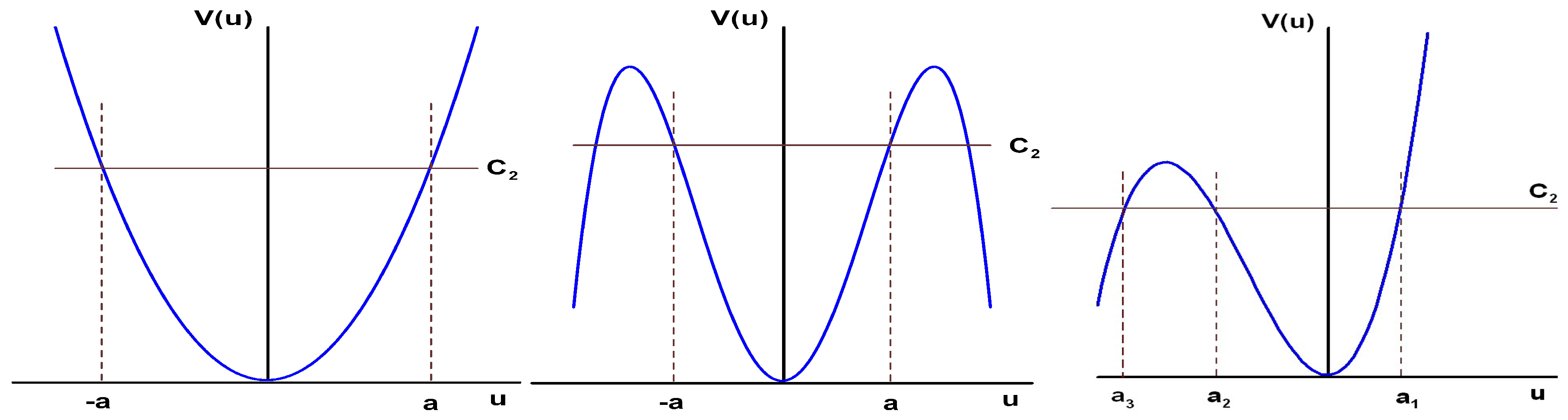
Let us consider (1) and its traveling wave solution as function of argument $\theta =\omega t-kx$. In this case Equation (1) can be transformed to

$$\omega \frac{\mathbf{d}u}{\mathbf{d}\theta }-k^3\frac{{\mathbf{d}}^{3}u}{\mathbf{d}{\theta }^3}=\frac{sk}{p+1}\frac{\mathbf{d}{u}^{p+1}}{\mathbf{d}\theta }.$$

(2)

After integrating (2) twice over $\theta$ we get

$$\omega u-k^3\frac{{\mathbf{d}}^{2}u}{\mathbf{d}{\theta }^2}=\frac{sk}{(p+1)}{u}^{p+1}-\frac{C_1}{2},$$

(3)

$$k^3{\left(\frac{\mathbf{d}u}{\mathbf{d}\theta }\right)}^2-\omega u^2+\frac{2sk}{(p+1)(p+2)}{u}^{p+2}=C_{1}u+C_2,$$

(4)

and the general solution to (1) can readily be written out in quadratures as

$$\theta -{\theta }_0=\pm k^{3/2}\int \frac{\mathbf{d}u}{\sqrt{C_{1}u+C_2+\omega u^2-\frac{2sk}{(p+1)(p+2)}{u}^{p+2}}}.$$

(5)

Here $C_1$ and $C_2$ are constants. To facilitate the understanding of the character of the solution (5) let us regard in on the phase plane and re-write Equation (4) as

$$k^3{\left(\frac{\mathbf{d}u}{\mathbf{d}\theta }\right)}^2+V\left(u\right)=C_2,$$

(6)

where

$$V\left(u\right)=-C_{1}u-\omega u^2+\frac{2sk}{(p+1)(p+2)}{u}^{p+2}.$$

(7)

Accordingly, it is easy to see that the function $V\left(u\right)$ may be regarded as potential energy, while the constant $C_2$ plays the role of total energy (defined by initial conditions, see above). In fact, the potential energy has only two free parameters—$C_1$ and frequency $\omega$, while the wave number k can be eliminated by scaling. The meaning of the parameter $C_1$ is also evident. If $C_1\ne 0,$ the term $C_{1}u$ in the potential $V\left(u\right)$ shifts its local extremum from zero to some nonzero level called pedestal. Further on we will only study the waves which are oscillating about zero, otherwise, a suitable scaling could be performed in the initial equation. Accordingly, without loss of generality we may put $C_1=0$ which yields

$$V\left(u\right)=-\omega u^2+\frac{2sk}{(p+1)(p+2)}{u}^{p+2}.$$

(8)

For waves with a small amplitude the second term can be neglected and (8) describes a linear case if the linear dispersion relation $\omega =-k^3$ is valid (i.e., frequency should be negative), with the obvious solution $u=acos\theta$.

If the second term in (8) is taken into account, this equation describes an anharmonic oscillator (the frequency is still regarded to be negative) and the form of the potential depends on the sign of the nonlinearity s and on whether p is odd or even.

Indeed, if $p=2n$ and $s=+1$, the potential has a parabolic-like shape shown in Figure 1, upper panel, with all solutions being periodic and symmetric. The amplitude of the nonlinear wave can be found from the condition

$$V\left(u\right)=C_2,$$

(9)

which determines two real roots a and $-a$ and $2(n-1)$ imaginary roots. If $s=-1$ and p is still even, the potential function changes its parabolic shape to a more complicated one, similar to a two-humped camel’s back shown in Figure 1, middle panel. In this case, the pit in the middle corresponds to the case of small amplitudes and the humps on the sides—to big amplitudes. Accordingly, waves do exist only for bounded magnitudes of amplitudes that can be found from the condition

$$V{\left(u\right)}_{max}<C_2.$$

(10)

In this case, there are four real roots of the Equation (9) but the amplitude is defined by those two roots that are in the neighborhood of the axes $u=0$.

Now, let us consider the case when $p=2n+1$ and $s=+1$ displayed in Figure 1, lower panel. In this case periodic solutions in the form of traveling waves do exist for the bounded magnitude of amplitudes satisfying (10). Indeed, Equation (9) has three real roots $a_1>0,a_2<0,a_3<0$, and oscillations take place $a_1$ and $a_2$. Last case with $s=-1$ and $p=2n+1$ is easily obtained from the above by the mirrored reflection about the vertical axis yielding change of signs in all roots, and are not shown in Figure 1.

Completing this section we conclude that

(a)

solutions to (1) in the form of periodic traveling waves do exist for an arbitrary sign of the nonlinearity in (1); and

(b)

they are symmetric with respect to horizontal axes for even powers of the nonlinearity, i.e., $p=2n,n=1,2,\dots$, and asymmetric for odd powers of the nonlinearity, $p=2n-1$.

For the well-known Korteweg-de Vries equation ($p=1$) and the modified Korteweg-de Vries equation ($p=2$), the (5) can be computed explicitly, e.g., for $p=1$ the solution reads

$$\begin{array}{ccc}\hfill u\left(\theta \right)& =& a\left[\frac{1-m}{m}-\frac{E\left(m\right)}{mK\left(m\right)}+{\mathbf{cn}}^2\left(\frac{K\left(m\right)\theta }{\pi };m\right)\right],\hfill \\ \hfill \frac{\omega }{k}& =& \frac{sa}{3}\left[\frac{2-m}{m}-\frac{3E\left(m\right)}{mK\left(m\right)}\right],\hfill \end{array}$$

where a is a wave amplitude, $\mathbf{cn}(x;m)$ is the Jacobian elliptic function of modulus $m,0<m<1,$ which is double periodic in $\theta$, and $K\left(m\right)$ is elliptic integral of the first order.

However, usually we can substantiate with some nice analytical expression neither the shape of the traveling wave nor the dispersion function which governs it from (5). Therefore, further on we introduce a small parameter and use the perturbation technics which allows construction of an explicit form of the approximate solution to (1), under the assumption that the nonlinearity is small.

Expansions like this have been rigorously justified in many contexts, e.g., in the framework of the reduced Ostrovsky equation with quadratic and cubic nonlinearity, see details in [29].

3. Frequency Correction, Symmetric Case

In this section we compute the nonlinear frequency correction $\mathsf{\Omega }$ which appearing in the dispersion of a symmetric traveling wave due to the weak nonlinearity in the even power, i.e., for $p=2n$. Let us first regard even values of p where $p=2n,n=1,2,\dots$. As our goal is to investigate weakly nonlinear wave packets, we can rewrite (1) using a small parameter $0<\epsilon \ll 1$ as follows

$$u_t+u_{xxx}=-\epsilon s{u}^{2n}{u}_x=-\frac{s\epsilon }{2n+1}{u}_x^{2n+1}$$

(11)

and look for a solution in the form

$$u\left(\theta \right)=acos\theta +\epsilon u_1\left(\theta \right)+\mathcal{O}\left({\epsilon }^2\right)+\dots ;$$

(12)

$$\theta =\omega t-kx;$$

(13)

$$\omega =-k^3+\epsilon \mathsf{\Omega }+\mathcal{O}\left({\epsilon }^2\right)+\dots ,$$

(14)

where a and k are wave amplitude and wave vector of linear monochromatic wave while other terms are induced by the small nonlinearity.

Let us substitute (12) into (11) and make equal the terms of the first order on small parameter $\epsilon$. This yields the ordinary differential equation of the second order:

$$-k^3(\frac{{\mathbf{d}}^2{u}_1}{\mathbf{d}{\theta }^2}+u_1)=-a\mathsf{\Omega }cos\theta +\frac{sk{a}^{2n+1}}{2n+1}{cos}^{2n+1}\theta ,$$

(15)

where constant of integration is chosen to be zero providing no perturbation for $a=0$. Now we substitute the Fourier series of the function ${cos}^{2n+1}\theta$ into the differential equation above; the result may be written out as

$${cos}^{2n+1}\theta =\frac{1}{2^{2n}}\left[\left(\genfrac{}{}{0pt}{}{2n+1}{n}\right)cos\theta +\sum _{m=0}^{n-1}\left(\genfrac{}{}{0pt}{}{2n+1}{m}\right)cos\left[\right(2n-2m+1)\theta ]\right],$$

(16)

where $\left(\genfrac{}{}{0pt}{}{n}{m}\right)$ are binomial coefficients (here and below we use the standard series presentations from [30]). The term with $cos\theta$ is separated from the other sum to facilitate the standard Poincaré procedure of eliminating of the resonance terms in a nonlinear ordinary differential equation (ODE) (for more detail see e.g., [31], p. 8).

The right hand side (RHS) of (15) is a superposition of Fourier harmonics with numbers $1,2,\cdots ,(2n+1)$, however the left hand side (LHS) may have resonance only with the first harmonics. Accordingly, the first harmonic term in the RHS of (15) will induce the secular grow of nonlinear correction $u_1$. Taking into account the uncertainty of the frequency correction $\mathsf{\Omega }$, we choose to eliminate resonance terms in (15) which yields

$$\mathsf{\Omega }=\frac{sk}{(2n+1)2^{2n}}\left(\genfrac{}{}{0pt}{}{2n+1}{n}\right)a^{2n}=s{B}_{n}k{a}^{2n},$$

(17)

where

$$B_n=\frac{\left(2n\right)!}{4^{n}n!(n+1)!}.$$

(18)

Obviously, $B_n>0$ for arbitrary n and accordingly the sign of the nonlinear correction to the wave frequency coincides the sign of s.

Direct substitution of (17) into (13) yields a bounded solution for $u_1$ to the basic wave of the form

$$u_1(cos\theta )=\sum _{m=0}^{n-1}{A}_{m}cos\left[\right(2n+1-2m\left)\theta \right],$$

(19)

where

$$\begin{array}{ccc}\hfill A_m& =& \frac{s{a}^{2n+1}}{k^2}\frac{\left(2n\right)!}{4^n}{T}_m,\hfill \\ \hfill T_m& =& \frac{1}{m!(2n+1-m)![{(2n+1-2m)}^2-1]}.\hfill \end{array}$$

(20)

Thus, the first order frequency correction of the weakly nonlinear wave is completely defined.

Some straightforward considerations allow us to make some qualitative estimations the Fourier spectrum (19). Indeed, for integers $m,n$ the coefficient $T_m<1,\forall m\le n-1$. Moreover, regard the ratio of two consequent Fourier coefficients $A_m/A_{m+1}$:

$$\begin{array}{ccc}\hfill {\rho }_m& =& \frac{A_m}{A_{m+1}}=\frac{T_m}{T_{m+1}}\hfill \\ & =& \frac{(m+1)!(2n+1-(m+1))![{(2n+1-2(m+1))}^2-1]}{m!(2n+1-m)![{(2n+1-2m)}^2-1]}\hfill \\ & =& \frac{(m+1)[{(2n+1-2(m+1))}^2-1]}{(2n+1-m)[{(2n+1-2m)}^2-1]}\hfill \\ & =& \frac{(m+1)}{(2n+1-m)}\frac{{(2n+1-2(m+1))}^2-1}{{(2n+1-2m)}^2-1}.\hfill \end{array}$$

(21)

The first fraction in (21) is increasing from $1/(2n+1)$ to $n/(n+2)$ and at the same time staying less than 1. The second fraction in (21) is also less than 1 while $2n+1-2(m+1)<2n+1-2m$. Accordingly, for fixed n coefficients $A_m$ in (19) increase with the increasing of m, namely $A_m<A_{m+1},\forall m\le n-1.$ This means that the amplitudes of the excited harmonics of the higher order (small m) decrease when increasing the number of harmonics.

4. Frequency Correction, Asymmetric Case

In this section we compute the nonlinear frequency correction $\mathsf{\Omega }$ appearing in asymmetric solutions to (1) with $p=2n-1$. Let $p=2n-1$ and introduce a small parameter $0<\epsilon \ll 1$ as above, then (1) can be rewritten as

$$u_t+u_{xxx}=-\epsilon s{u}^{2n-1}{u}_x=-\frac{\epsilon s}{2n}{u}_x^{2n}$$

(22)

and using the phase presentation as above, $\theta =\omega t-kx$, one can easily deduce an ODE similar to (15) which after integration over $\theta$ yields

$$\omega \frac{\mathbf{d}u}{\mathbf{d}\theta }-k^3\frac{{\mathbf{d}}^{3}u}{\mathbf{d}{\theta }^3}=\frac{\epsilon sk}{2n}{u}^{2n}.$$

(23)

Now the wave traveling solution is searched for in the form

$$u\left(\theta \right)=U\left(\theta \right)+\epsilon u_1\left(\theta \right)+{\epsilon }^2{u}_2\left(\theta \right)+\mathcal{O}\left({\epsilon }^3\right)+\dots ,$$

(24)

$$U\left(\theta \right)=acos\theta ,$$

(25)

$$\omega =-k^3+\epsilon {\mathsf{\Omega }}_1+{\epsilon }^2{\mathsf{\Omega }}_2+\mathcal{O}\left({\epsilon }^3\right)+\dots$$

(26)

Beginning with equaling terms in the first order on $\epsilon$ we deduce

$$\begin{array}{ccc}\hfill -k^3\left[\frac{{\mathbf{d}}^2{u}_1}{\mathbf{d}{\theta }^2}+u_1\right]& =& \frac{sk}{2n}{U}^{2n}-{\mathsf{\Omega }}_{1}U\hfill \\ & =& \frac{sk}{2n}{a}^{2n}{cos}^{2n}\theta -{\mathsf{\Omega }}_{1}acos\theta .\hfill \end{array}$$

(27)

The general reasoning in this section is analogous to the approach described above. However, as in this case first order terms do not generate secular terms, we have to consider also terms of the second order on $\epsilon$.

As

$${cos}^{2n}\theta =\sum _{m=0}^n{D}_{m}cos\left[2\right(n-m\left)\theta \right]$$

(28)

with positive coefficients given by

$$D_m=\frac{1}{2^{2n-1}}\left(\genfrac{}{}{0pt}{}{2n}{m}\right),\forall m=0,1,\dots ,n-1;$$

(29)

$$D_n=\frac{1}{2^{2n}}\left(\genfrac{}{}{0pt}{}{2n}{n}\right).$$

(30)

Notice that the Fourier series (28) does not contain terms which are in resonance with the LHS of (27) and without loss of generality we may choose ${\mathsf{\Omega }}_1=0$; this yields the bounded solution

$$u_1=\sum _{m=0}^n{\tilde{A}}_{m}cos\left[2\right(n-m\left)\theta \right],$$

(31)

$${\tilde{A}}_m=\frac{s{a}^{2n}}{2n{k}^2}\frac{D_m}{4{(n-m)}^2-1}.$$

(32)

It is important to notice that the sign of the Fourier coefficient $A_m$ coincides with the sign of s for all $m<n$ and is opposite if $m=n$. The last case corresponds to the mean level in the nonlinear wave and is characterized as follows:

$${\tilde{A}}_n=\frac{s{a}^{2n}}{6n{k}^2}{D}_n.$$

(33)

Notice that solution of (1) is defined up to the constant which can be easily excluded from consideration, similar to what has been done in (7). On the other hand, this constant will affect the nonlinear frequency correction. Therefore, first we regard waves with zero mean level omitting this constant (pedestal) but at the end of this section we also compute the constant.

4.1. Case A: Zero Mean Level

After omitting ${\tilde{A}}_n$, the Equation (31) is reduced to

$$u_1=\sum _{m=0}^{n-1}{\tilde{A}}_{m}cos\left[2\right(n-m\left)\theta \right],$$

(34)

and in the next order of perturbation theory we have

$$\begin{array}{ccc}\hfill -k^3\left[\frac{{\mathbf{d}}^2{u}_2}{\mathbf{d}{\theta }^2}+u_2\right]& =& sk{U}^{2n-1}{u}_1-\mathsf{\Omega }U\hfill \\ & =& sk{a}^{2n-1}{u}_1{cos}^{2n-1}\theta -\mathsf{\Omega }acos\theta .\hfill \end{array}$$

(35)

It follows from (31) and (32) that $u_1$ contains s as a factor and as $s^2=1$, we may omit s in (35). The use of standard series

$${cos}^{2n-1}\theta =\sum _{l=0}^{n-1}{F}_{l}cos\left[(2n-2l-1)\theta \right],$$

(36)

$$F_l=\frac{1}{4^{n-1}}\left(\genfrac{}{}{0pt}{}{2n-1}{l}\right)$$

(37)

together with (31) allows us to rewrite the first term of the RHS of (35) $cos\theta$ as

$$\begin{array}{ccc}\hfill k{a}^{2n-1}{u}_1{cos}^{2n-1}\theta & =& k{a}^{2n-1}\hfill \\ & \times & \sum _{m=0}^{n-1}\sum _{l=0}^{n-1}{\tilde{A}}_m{F}_{l}cos\left[2\right(n-m\left)\theta \right]cos\left[(2n-2l-1)\theta \right]\}\hfill \\ & =& \frac{k{a}^{2n-1}}{2}\sum _{m=0}^{n-1}\sum _{l=0}^{n-1}{F}_m{\tilde{A}}_l\hfill \\ & \times & \{cos[(4n-2l-2m-1)\theta ]+cos[(2m-2l+1)\theta \left]\right\}\hfill \end{array}$$

(38)

Looking for the terms being in resonance with (38) in the form

$$\begin{array}{c}\hfill \frac{k{a}^{2n-1}}{2}cos\theta \left(\sum _{m=0}^{n-1}{F}_m{\tilde{A}}_m\right)\end{array}$$

we rewrite them as

$$\begin{array}{c}\hfill \frac{k{a}^{2n-1}}{2}cos\theta ·I_n,I_n=\sum _{m=0}^{n-1}{F}_m{\tilde{A}}_m.\end{array}$$

(39)

Accordingly, condition of the absence of resonance in (35) yields

$${\mathsf{\Omega }}_{2,1}=\frac{k{a}^{2n-2}}{2}{I}_n,$$

(40)

which is the nonlinear frequency correction for the periodic wave in the case of zero mean flow. It follows from (33) and (39) that the sign of ${\mathsf{\Omega }}_{2,1}$ coincides with the sign of s.

4.2. Case B: Non-Zero Mean Level

In this case, we have to consider not pure periodic waves but wave packets with amplitudes slowly changing in time and in space. As a result, in the asymmetric case a flow is induced which moves with the wave packet. For computing the induced flow let us first average (1) over wavelength:

$$<u{>}_t+\frac{s}{p+1}<u^{p+1}{>}_x=0.$$

(41)

Taking into account that $u=acos\theta$ in the zero approximation, the mean value $<u^{p+1}>=0$ for even $p=2n$ and no induced wave packet occurs in the symmetrical case. On the other hand, for $p=2n-1$ we get

$$<u^{p+1}>=a^{2n}<{cos}^{2n}\theta >=a^{2n}{D}_n$$

(42)

and averaged wave amplitude is not constant anymore, $<u{>}_x\ne 0.$ In the first approximation, the linear wave packet is moving with the linear group velocity $c_{gr}=-\mathbf{d}\omega /\mathbf{d}k=3k^2$ and consequently $a=a(x-c_{gr}t)$. This means that also induced wave packet ${\tilde{A}}_n$ is the function of the same variables, i.e.,

$${\overline{A}}_n=s{\tilde{A}}_n,{\tilde{A}}_n=-\frac{a^{2n}}{3k^2}{D}_n$$

(43)

and the nonlinear frequency correction due to the non-zero mean level can only be computed as follows (similar to the previous case):

$${\mathsf{\Omega }}_{2,2}=-\frac{k{a}^{2n-2}}{2}\frac{a^{2n}}{3k^2}{D}_n$$

(44)

It is easy to see that ${\mathsf{\Omega }}_{2,2}<0$ is always negative.

4.3. Total Frequency Correction

A combination of (40) and (44) yields the final expression for the nonlinear correction $\mathsf{\Omega }$ in the asymmetric case

$${\mathsf{\Omega }}_2={\mathsf{\Omega }}_{2,1}+{\mathsf{\Omega }}_{2,2}=\frac{k{a}^{2n-2}}{2}(I_n-\frac{a^{2n}}{3k^2}{D}_n)$$

(45)

and our last task is to estimate whether ${\mathsf{\Omega }}_2$ is positive or negative.

As the sign of ${\mathsf{\Omega }}_{2,1}$ coincides with the sign of s and ${\mathsf{\Omega }}_{2,2}$ is always negative, we conclude immediately that nonlinear frequency correction for ${\mathsf{\Omega }}_2$ is negative for $p=2n-1$ and $s=-1$.

On the other hand, from $s=+1$ it follows that each term of the sum $I_n={\sum }_{m=0}^{n-1}{F}_m{\tilde{A}}_m$ is positive. To define the sign of ${\mathsf{\Omega }}_2$ let us compare $a^{2n}/3k^2{D}_n$ with one term of this sum corresponding to $m=n-1$, i.e., ${\tilde{A}}_{n-1}{F}_{n-1}$. The use of formulae (29) and (30) for $D_m$ and $D_n$, expression (37) for $F_m$ and (43) for ${\tilde{A}}_n$ yields

$$\begin{array}{c}\hfill \frac{a^{2n}}{3k^2}{D}_n=\frac{a^{2n}}{3k^2}\frac{1}{3}\frac{1}{2^{2n}}\frac{\left(2n\right)!}{n!n!};\\ \hfill {\tilde{A}}_{n-1}{F}_{n-1}=\frac{a^{2n}}{3k^2}{D}_{n-1}{F}_{n-1}=\frac{a^{2n}}{3k^2}\frac{1}{2^{2n-1}}\frac{\left(2n\right)!}{(n-1)!(n+1)!}{F}_{n-1}=\end{array}$$

(46)

$$\begin{array}{c}\hfill \frac{a^{2n}}{3k^2}\frac{1}{2^{2n-1}}\frac{n\left(2n\right)!}{n!n!(n+1)}\frac{(2n-1)!}{n(n-1)};\end{array}$$

(47)

$$\begin{array}{c}\hfill F_{n-1}{\tilde{A}}_{n-1}-\frac{a^{2n}}{3k^2}{D}_n=\frac{a^{2n}}{3k^2}\frac{1}{2^{2n}}\frac{\left(2n\right)!}{n!n!}[\frac{2(2n-1)!}{(n-1)(n+1)}-\frac{1}{3}].\end{array}$$

(48)

Direct computation shows that for $n=1$ function $[2(2n-1)!/(n-1)(n+1)]>1$ and according to Stirling’s approximation

$$n!\sim \sqrt{2\pi n}{\left(\frac{n}{e}\right)}^n,$$

(49)

this is a fast growing function of order of $n^{n-3/2}$, i.e., the bracket (46) is always positive,

$$[\frac{2(2n-1)!}{(n-1)(n+1)}-\frac{1}{3}]>0\forall n.$$

(50)

Thus it was demonstrated that the nonlinear frequency correction ${\mathsf{\Omega }}_2$ is positive for $p=2n-1$ and $s=1$.

$$\begin{array}{c}\hfill {\mathsf{\Omega }}_2={\mathsf{\Omega }}_{2,1}+{\mathsf{\Omega }}_{2,2}=\frac{k{a}^{2n-2}}{2}(I_n-\frac{a^{2n}}{3k^2}{D}_n)=\\ \hfill \frac{k{a}^{2n-2}}{2}(\sum _{m=0}^{n-1}{F}_m{\tilde{A}}_m-\frac{a^{2n}}{3k^2}{D}_n)=\\ \hfill \frac{k{a}^{2n-2}}{2}(\sum _{m=0}^{n-1}{F}_m\frac{s{a}^{2n}}{2n{k}^2}\frac{D_m}{4{(n-m)}^2-1}-\frac{a^{2n}}{3k^2}{D}_n)=\\ \hfill \frac{a^{4n-2}}{2nk}(s\sum _{m=0}^{n-1}{F}_m\frac{1}{2}\frac{D_m}{4{(n-m)}^2-1}-\frac{n}{3}{D}_n)=\\ \hfill \frac{a^{4n-2}}{2nk}(s\sum _{m=0}^{n-1}\frac{1}{2^{2n-1}}\left(\genfrac{}{}{0pt}{}{2n-1}{m}\right)\frac{D_m}{4{(n-m)}^2-1}-\frac{n}{3}{D}_n)\Rightarrow {\mathsf{\Omega }}_2=\frac{a^{4n-2}}{k}\widetilde{B_n},\end{array}$$

(51)

where

$$\widetilde{B_n}=s\sum _{m=0}^{n-1}\frac{1}{n{2}^{2n-1}}\left(\genfrac{}{}{0pt}{}{2n-1}{m}\right)\frac{D_m}{4{(n-m)}^2-1}-\frac{1}{6}{D}_n.$$

(52)

and $D_m,D_n$ are given by (29) and (30).

5. Modified NLS Equations

The knowledge of the explicit form of the dispersion relation allows us to write out the corresponding NLS equation without using an asymptotic procedure. Indeed,

$$\omega -{\omega }_0=c_{gr}(k-k_0)+\frac{1}{2}\frac{{\mathbf{d}}^2\omega }{\mathbf{d}{k}^2}(k-k_0^2)+\mathsf{\Omega }.$$

(53)

and the use of the standard operator equalities

$$a_T\leftrightarrow i(\omega -{\omega }_0)a,\mathrm{and}{a}_X\leftrightarrow -i(k-k_0)a$$

(54)

and the expression for $\mathsf{\Omega }$ given by (17) allows us finally to obtain the modified NLS equation in general form for the symmetrical case, i.e., for even power $p=2n$:

$$i{a}_T+3k{a}_{XX}+sk{B}_n{\left|a\right|}^{2n}a=0,B_n=\frac{\left(2n\right)!}{4^{n}n!(n+1)!}.$$

(55)

For $n=1$ the equation above coincides with classical NLS equation which is focusing for $s=1$ and defocusing otherwise.

The modified NLS equation in the asymmetric case, i.e., with $p=2n-1$, has the form

$$i{a}_T+3k{a}_{XX}+\frac{1}{k}\widetilde{B_n}{\left|a\right|}^{4n-2}a=0$$

(56)

with $\widetilde{B_n}$ given by (52). In this case, s is hidden in $\widetilde{B_n}$ and it was demonstrated above that $\widetilde{B_n}>0$ if $s=1$ and $\widetilde{B_n}<0$ otherwise.

The Equation (56) looks quite similar to the Equation (55), differing only in the form of the coefficients in front of the nonlinear term. Both equations have the same structure and their nonlinear terms have both the even power.

Analysis of modulational instability for the focusing case $s=1$ yields the explicit expression for the instability increment

$$\Gamma =\sqrt{3a_0}K\sqrt{2n{B}_n{a}_0^{2n}-3K^2}.$$

(57)

Maximal increment ${\Gamma }_{max}$,

$${\Gamma }_{max}=n{B}_n{a}_0^{2n},$$

(58)

is achieved at the wave number $K_{max}$,

$$K_{max}=\sqrt{\frac{n{B}_n}{3}}{a}_0^n,$$

(59)

and the boundary wave number of the envelope $K_b$ is

$$K_b=\sqrt{2}{K}_{max}.$$

(60)

6. Discussion

• We have deduced the constructive condition for the occurrence of modulational instability in the class of the higher order KdV equations $u_t+s{u}^p{u}_x+u_{xxx}=0$ with an arbitrary positive integer p. We demonstrated constructively that for $p>2$ the weakly modulated wave train is described by the high-order NLS equation whose solutions are stable for both even and odd p if $s=-1$. Notice that in the known literature examples of studying stability of solutions to specific equations of this class by other methods, e.g., [25,28], yield results depending on the the sign of a pedestal.
  It is important to realize that in the frame of the KdV-family of equations, the Fourier mode $A_n$ describes the wave-induced mean flow term. In the symmetric case this fact does not influence the form of the nonlinear frequency correction obtained in Section 3 while in the asymmetric case it will contribute into the nonlinear term in the NLS equation. The influence of the zero harmonic requires a special wave-mean flow analysis which has been explicitly performed in this paper.
  Some other substantial differences between symmetric and asymmetric cases are demonstrated below.
• For deducing the conditions of the instability, we first computed the nonlinear corrections to the frequency of the Stokes wave and then explored the coefficients of (m)NLS equations obtained, thus deducing explicit expressions for the instability growth rate, maximum of the increment and the boundaries of the instability interval. These results can be used for planning numerical and laboratory experiments similar to [15,16], and for explaining the available data, e.g., [22,23]. An important issue here would be to choose small parameters and initial amplitudes facilitating these results which is not a simple problem. The approximations of a solution of gKdV equations by solutions of gNLS equations are the subject of a few tedious mathematical studies (see e.g., [32] and the bibliography therein), where it is rigorously proven that the quality of approximation depends not only on p and s but also on the parameters of the initial excitation.
• We have shown that conditions of the modulational instability have different forms depending on whether p is an even number (symmetric case) or odd number (asymmetric case) where the words symmetric and asymmetric are used loosely referring to the form of the corresponding solutions, as discussed in Section 2. An interesting mathematical fact is that the properties of the corresponding NLS-family of equations are also different. Namely,

  (a)

  In the symmetric case the nonlinear terms have the same power $p=2n$ both in the initial (m)KdV equation and corresponding (m)NLS equation; this means in particularly that (m)NLS equations with an odd power of nonlinearity, for instance

  $$i{a}_T+3k{a}_{XX}+\mathrm{const}{\left|a\right|}^{3}a=0$$

  (61)

  can not appear this way.

  (b)

  in the asymmetric case starting with different higher order KdV equations one can come to the same (m)NLS equation. Further on we call these couples of equations an associate pair. The first trivial associate pair reads

  $$u_t+su{u}_x+u_{xxx}=0,u_t+s{u}^2{u}_x+u_{xxx}=0$$

  (62)

  and both equations are reduced to the classical NLS equation

  $$i{a}_T+3k{a}_{XX}+\mathrm{const}{\left|a\right|}^{2}a=0.$$

  (63)

  More interesting example of a non-trivial associated pair is given by equations

  $$u_t+s{u}^3{u}_x+u_{xxx}=0,u_t+s{u}^6{u}_x+u_{xxx}=0$$

  (64)

  that can be reduced to

  $$i{a}_T+3k{a}_{XX}+\mathrm{const}{\left|a\right|}^{6}a=0.$$

  (65)

  An associated pair consist of one symmetric and one asymmetric (m)KdV equation.

  (c)

  In asymmetric case, each (m)KdV equation belongs to some associated pair.

  (d)

  In symmetric case, there are single (m)KdV equations which do not belong to any associated pair, for example, equation

  $$u_t+s{u}^4{u}_x+u_{xxx}=0$$

  (66)

  is single and generates (m)NLS of the form

  $$i{a}_T+3k{a}_{XX}+\mathrm{const}{\left|a\right|}^{4}a=0.$$

  (67)

  All these properties point indicate an existence of different inner structures of the NLS-families appearing in symmetrical and asymmetrical cases which deserves a special study. The existence of associated pair might also imply a corresponding physical interpretation. These issues are presently under study.

References

1. Kurkina, O.E.; Kurkin, A.A.; Soomere, T.; Pelinovsky, E.N.; Ruvinskaya, E.A. Higher-order (2+4) Korteweg-de Vries—Like equation for interfacial waves in a symmetric three-layer fluid. Phys. Fluids 2011, 23, 116602. [Google Scholar] [CrossRef]
2. Kurkina, O.E.; Kurkin, A.A.; Ruvinshaya, E.A.; Pelinovsky, E.N.; Soomere, T. Dynamics of solitons in a nonintegrable version of the modified Korteweg-de Vries equation. JETP Lett. 2012, 95, 91–95. [Google Scholar] [CrossRef]
3. Rudenko, O.V. Modular solitons. Dokl. Math. 2016, 94, 708–711. [Google Scholar] [CrossRef]
4. Nazarov, V.E.; Kiyashko, S.B.; Radostin, A.V. Stationary waves in a bimodular rod of finite radius. Wave Motion 2017, 75, 72–76. [Google Scholar] [CrossRef]
5. Chatterjee, A. Asymptotic solution for solitary waves in a chain of elastic spheres. Phys. Rev. E 1999, 59, 5912–5919. [Google Scholar] [CrossRef]
6. James, G.; Pelinovsky, D.E. Gaussian solitary waves and compactons in Fermi-Pasta-Ulam lattices with Hertzian potentials. Proc. R. Soc. A 2014, 470, 20130465. [Google Scholar] [CrossRef]
7. Dumas, E.; Pelinovsky, D.E. Justification of the log-KdV equation in granular chains: The case of precompression. SIAM J. Math. Anal. 2014, 46, 4075–4103. [Google Scholar] [CrossRef]
8. Pelinovsky, D.E.; Giniyatullin, A.R.; Panfilova, Y.A.; Shurgalina, E.G.; Rodin, A.A. Analytical approximations of solitary waves in granular crystals. Trans. Nizhni Novgorod State Tech. Univ. R.Y. Alexeev 2013, 100, 55–69. (In Russian) [Google Scholar]
9. Martel, Y.; Merle, F. Instability of solitons for the critical generalized Korteweg-de Vries equation. GAFA Geom. Funct. Anal. 2001, 11, 74–123. [Google Scholar] [CrossRef]
10. Martel, Y.; Merle, F. Asymptotic stability of solitons of the gKdV equations with general nonlinearity. Math. Ann. 2008, 341, 391–427. [Google Scholar] [CrossRef]
11. Klein, C.; Peter, R. Numerical study of blow-up and dispersive shocks in solutions to generalized Korteweg-de Vries equations. Physica D 2015, 304–305, 52–78. [Google Scholar] [CrossRef]
12. Zakharov, V.E.; Kuznetsov, E.A. Multi-scale expansions in the theory of systems integrable by the inverse scattering transform. Physica D 1986, 18, 455–463. [Google Scholar] [CrossRef]
13. Grimshaw, R.; Pelinovsky, D.; Pelinovsky, E.; Talipova, T. Wave group dynamics in weakly nonlinear long-wave models. Physica D 2001, 159, 35–57. [Google Scholar] [CrossRef]
14. Grimshaw, R.; Pelinovsky, E.; Talipova, T.; Ruderman, M.; Erdelyi, R. Short-lived large-amplitude pulses in the nonlinear long-wave model described by the modified Korteweg-de Vries equation. Stud. Appl. Math. 2005, 114, 189–210. [Google Scholar] [CrossRef]
15. Ruderman, M.S.; Talipova, T.; Pelinovsky, E. Dynamics of modulationally unstable ion-acoustic wave packets in plasmas with negative ions. J. Plasma Phys. 2008, 74, 639–656. [Google Scholar] [CrossRef]
16. Grimshaw, R.; Pelinovsky, E.; Talipova, T.; Sergeeva, A. Rogue internal waves in the ocean: Long wave model. Eur. Phys. J. Spec. Top. 2010, 185, 195–208. [Google Scholar] [CrossRef]
17. Chowdury, A.; Ankiewicz, A.; Akhmediev, N. Periodic and rational solutions of modified Korteweg-de Vries equation. Eur. Phys. J. D 2016, 70, 104. [Google Scholar] [CrossRef]
18. Kartashova, E. Energy spectra of 2D gravity and capillary waves with narrow frequency band excitation. EPL 2012, 97, 30004. [Google Scholar] [CrossRef]
19. Kartashova, E. Energy transport in weakly nonlinear wave systems with narrow frequency band excitation. Phys. Rev. E 2012, 86, 041129. [Google Scholar] [CrossRef]
20. Kartashova, E. Time scales and structures of wave interaction exemplified with water waves. EPL 2013, 102, 44005. [Google Scholar] [CrossRef]
21. Tobisch, E. Energy spectrum of ensemble of weakly nonlinear gravity-capillary waves on a fluid surface. J. Exp. Theor. Phys. 2014, 119, 359–365. [Google Scholar] [CrossRef]
22. Dutykh, D.; Tobisch, E. Direct dynamical energy cascade in the modified KdV equation. Physica D 2015, 297, 76–87. [Google Scholar] [CrossRef]
23. Dutykh, D.; Tobisch, E. Observation of the inverse energy cascades in the modified Korteweg-de Vries equation. EPL 2014, 107, 14001. [Google Scholar] [CrossRef]
24. Whitham, G.B. Linear and Nonlinear Waves; Wiley Series in Pure and Applied Mathematics; Wiley: Hoboken, NJ, USA, 1999. [Google Scholar]
25. Bronski, J.C.; Hur, V.M.; Johnson, M.A. Modulational instability in equations of KdV type. In New Approaches to Nonlinear Waves; Tobish, E., Ed.; Springer: Berlin, Germany, 2015; pp. 79–125. [Google Scholar]
26. Minzoni, A.A.; Smyth, N.F. Modulation theory, dispersive shock waves and Gerald Beresford Whitham. Physica D 2016, 333, 6–10. [Google Scholar] [CrossRef]
27. El, G.E.; Hoefer, M.A. Dispersive shock waves and modulational theory. Physica D 2016, 333, 11–65. [Google Scholar] [CrossRef]
28. Tobisch, E.; Pelinovsky, E.N. Conditions for modulation instability in higher order Korteweg- de Vries equations. Appl. Math. Lett. 2018, 88, 28–32. [Google Scholar] [CrossRef]
29. Johnson, E.R.; Pelinovsky, D.E. Orbital stability of periodic waves in the class of reduced Ostrovsky equations. J. Diff. Equ. 2016, 261, 3268–3304. [Google Scholar] [CrossRef]
30. Gradshteyn, I.S.; Ryzhik, I.M.; Geronimus, Y.V.; Tseytlin, M.Y. Table of Integrals, Series, and Products; Academic Press: Cambridge, MA, USA, 1980. [Google Scholar]
31. Kartashova, E. Nonlinear Resonance Analysis: Theory, Computation, Applications; Cambridge University Press: Cambridge, UK, 2010. [Google Scholar]
32. Masaki, S.; Segata, J. Existence of a minimal non-scattering solution to the mass-subcritical generalized Korteweg-de Vries equation. Annales de l’Institut Henri Poincaré C Analyse non LinéAire 2018, 35, 283–326. [Google Scholar] [CrossRef]
Figure 1. Shape of of the potential V ( u ) = ω u 2 + 2 s k ( p + 1 ) ( p + 2 ) u p + 2 . Left panel: s = + 1 , p = 2 n . Middle panel: s = 1 , p = 2 n . Right panel: s = + 1 , p = 2 n + 1 .
Fluids 04 00054 g001