Abstract
A two-phase bubbly flow is often found in the process industry. For the efficient operation of such devices, it is important to know the details of the flow. The paper presents a numerical simulation of the rising bubble in a stagnant liquid column. The interFOAM solver from the open source Computational Fluid Dynamics (CFD) toolbox OpenFOAM was used to obtain the necessary data. The constant and dynamic computational grids were used in the numerical simulation. The results of the calculation were compared with the measured values. As expected, by using the dynamic mesh, the bubble trajectory was closer to the experimental results due to the more detailed description of the gas–liquid interface.
1. Introduction
Buoyancy-driven bubbly flow represents very demanding two-phase time-dependent three-dimensional flow, which is found in many natural and technological processes. Good knowledge of such flow is extremely important for the chemical and pharmaceutical industries where mixing vessels [1], bubble columns [2,3], and gas-lift reactors [4] can be found. In order to control the chemical reactions in these devices, the knowledge of the contact area between liquid and gas is crucial. The interfacial area depends on the flow regime or bubble size distribution. Another very important application of bubbly flow is in the field of heat transfer. Free-rising bubbles can cause the mixing of water layers with a temperature gradient, which is the so-called destratification [5], or increase heat transfer in heat exchanging devices by breaking the thermal boundary layer along the wall [6].
The complexity of the bubble flow represents a major challenge for theoretical, experimental, and numerical research. Sometimes it is very difficult to provide control over the experimental process and thus, obtaining accurate data due to the interference between the measuring probe and fluid flow can be challenging. Therefore, numerical simulation is increasingly used as a tool for the analysis of the bubbly flow [7,8,9].
The velocity fields of the two-phase flow can be significantly modified by the interfacial interactions, meaning that they must be taken into account through adequate closure laws. The determination of the interface depends on the considered problem. There are two approaches to describe the development of the interface. One is the interface tracking method [10] (Lagrangian), which is based on the use of markers on the interface. Another one is the interface capturing (Eulerian) method, which uses fixed mesh to solve the transport equation of the scalar quantity. Level-Set [11,12], Volume of Fluid (VOF) [13,14] and Euler–Euler [15,16] methods are representatives of this approach. When the bubble is substantially larger than the cell size of the computational grid, the VOF method is most commonly used. The drawback of this method is that we obtain a smearing interface when using the interpolation schemes of the lower order and the numerical oscillations when using higher order interpolation schemes. A possible solution involves the refinement of the computational mesh, but this requires a significant increase in computer resources (memory, computational time). This can be avoided by using the "Adaptive Mesh Refinement" (AMR) technique [17], in which the computational grid is refined only in the range of rapid changes in physical quantities (e.g., cells near the gas–liquid interface) and therefore, the computational mesh is dynamically changing as the refined mesh follows the movement of the bubble.
We have presented the numerical simulation of free-rising air bubble in a stagnant water column using constant (CM) and dynamic (DM) computational mesh in the following sections. The results are compared with experimental data obtained in the Laboratory for Fluid Dynamics and Thermodynamics during 1980–1992. The paper is organized as follows. In Section 2, the numerical model is described. The numerical simulation is presented in Section 3. In Section 4, the results of the simulation are presented and discussed. Finally, the conclusions are drawn in Section 5.
2. Numerical Model
2.1. Governing Equations
To determine the gas–liquid interface, we used the VOF method. The surface tension force was taken into account using the Continuum Surface Force (CSF) model [18]. Due to a low Reynolds number, the conditions were considered to be laminar. The time-dependent laminar incompressible two-phase flow can be described with the solution of the conservation equations:
- continuity
- momentum transportwhere α is the liquid volume fraction, ui is the velocity vector, p is the pressure, σij is the stress tensor due to the molecular viscosity, gi is the gravity acceleration vector, σ is the surface tension coefficient and κ is the gas–liquid interface curvature. Equation (1) and Equation (2) are connected through material properties. The mixture density ρ and mixture dynamic viscosity μ are determined by the following equations:where ρl and ρg are the liquid and gas density, whereas μl and μg are liquid and gas dynamic viscosity. The system of Equations (1)–(4) was solved within the OpenFOAM [19,20] toolkit, which has proven to be an effective tool for solving such problems [21].
Table 1 shows the material properties for air–water two-phase system, which was considered in our case.

Table 1.
Material properties.
2.2. Discrete Model
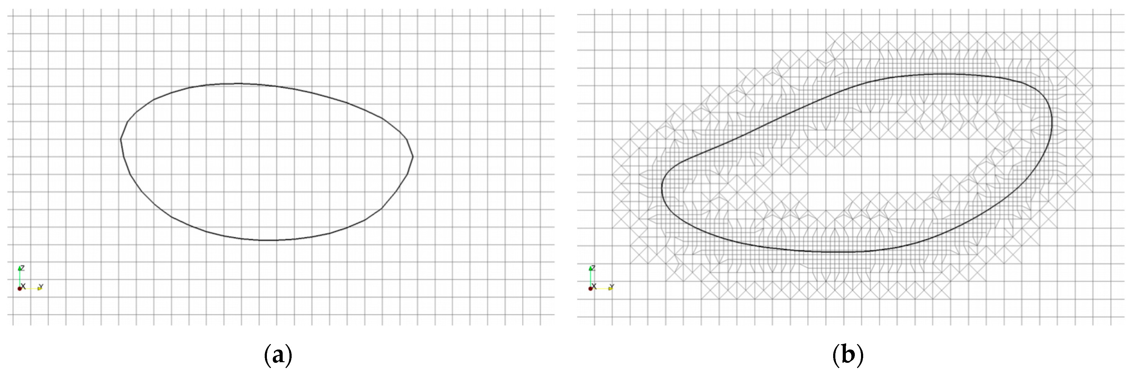
The computational domain is represented by a hexahedron with dimensions Lx = 40 mm, Ly = 80 mm and Lz = 290 mm (Figure 1). The domain is discretized with the structured computational grid. The number of cells in x, y and z coordinate directions is Nx = 100, Ny = 200 and Nz = 725. The total number of cells is 14.5 million and the size of individual cell is 0.4 mm. This mesh resolution is a consequence of the VOF two-phase flow simulation practice that there should be at least 15 cells per bubble diameter [5,22]. This recommendation applies in the case of constant computational mesh (Figure 2a). In the case of the dynamic mesh, the cell size varies in the part of computational domain according to the prescribed condition (e.g., 0.001 ≤ α ≤ 0.999). This means that cell is near gas–liquid interface (Figure 2b). The number of cells varied between 14.79 and 16.09 million.
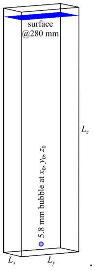
Figure 1.
Geometric model.
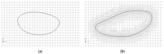
Figure 2.
Computational mesh: (a) Constant; (b) dynamic.
As an initial condition, we put a spherical bubble with a diameter of 5.8 mm at the bottom of the domain. The bubble center is located at coordinates x0 = 20 mm, y0 = 40 mm and z0 = 10 mm. The free surface occurs at the height H = 280 mm.
3. Numerical Simulation
The combination of the Pressure Implicit with Splitting of Operator (PISO) and Semi-Implicit Method for Pressure-Linked Equations (SIMPLE), which is the so-called PIMPLE algorithm, was used for velocity–pressure coupling [19,23]. The volume fraction, momentum and turbulence equations were solved with smoothSolver using symGaussSeidel smoother. For the pressure equation, we used Geometric Agglomerated Algebraic Multigrid (GAMG) solver with the Diagonal Incomplete-Cholesky (DIC) preconditioner for symmetric matrices.
The discretization schemes were:
- Euler explicit for the time derivative,
- Gauss linear for the gradient operator,
- Gauss upwind for the divergence operator
- Gauss linear corrected for the Laplacian operator.
We used the adjustable time step. This means that Δt was changed so that the Courant number did not exceed the prescribed value. In our simulation, we used the following maximum parameter values max(Co) = maxAlpha(Co) = 0.5 and consequently, the time step was varied between 1.2 × 10⁻³ s and 2.6 × 10⁻⁵ s with a constant mesh and 1.2 × 10⁻⁴ s and 7.0 × 10⁻⁶ s in the case of a dynamic mesh. The bubble reached the free surface in approximately 1.2 s. The velocity, pressure and volume fraction fields were saved every 0.02 s for post-processing purposes.
The calculations were carried out on Supermicro workstation (AMD Opteron 6136 2.4 GHz, 2 processors, 16 cores, 64 GB RAM, 8 TB disk). The "wall clock" time for a constant mesh was 3.2 days (8118 time steps) and for a dynamic mesh of 86 days (49210 time steps).
The difference is very large, but it is necessary to take two things into account:
- The division of computational cells increases the number of equations considerably.
- The Δt decreases due to the small cells and consequently increases the number of time steps.
4. Results and Discussion
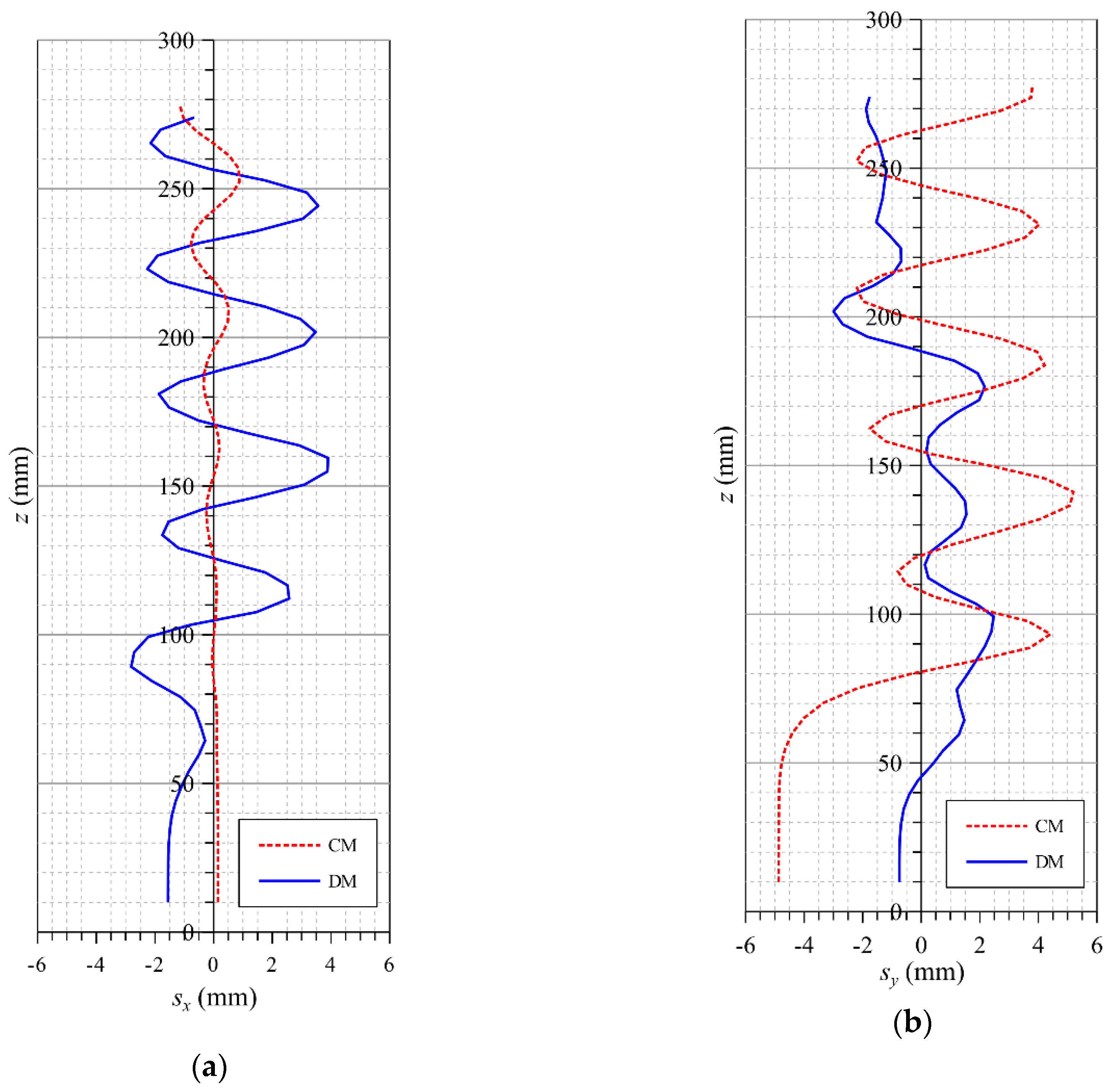
Figure 3 shows the trajectory of the bubble center or precisely the deviation and from the average value in x and y direction, respectively.
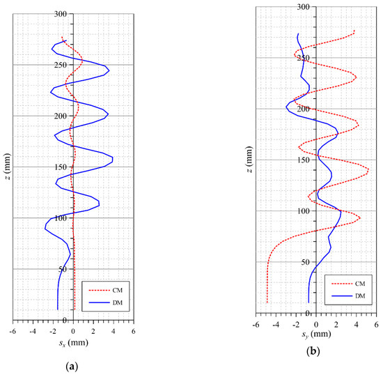
Figure 3.
Trajectory of the bubble center: (a) Front view; (b) side view.
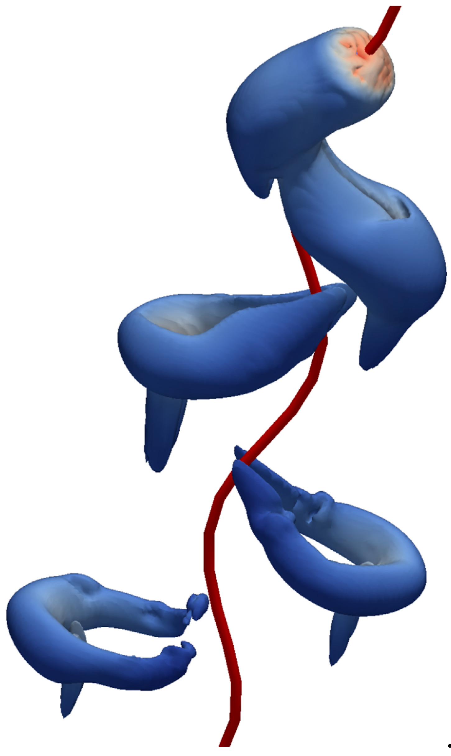
Initially, the stationary spherical bubble begins to move upwards due to the buoyancy force. As the bubble velocity rises, surface waves appear as a result of viscous friction and surface tension forces, which destroy symmetry and cause its shape to change from spherical to ellipsoidal. The bubble begins to wobble and travel along the spiral path, leaving behind the characteristic decaying vorticity structures [24], which is the so-called ‘horseshoe’ vortex (Figure 4), which further deforms its shape.
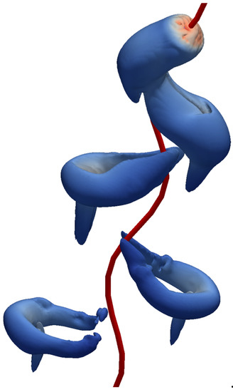
Figure 4.
Bubble path and vorticity structures for .
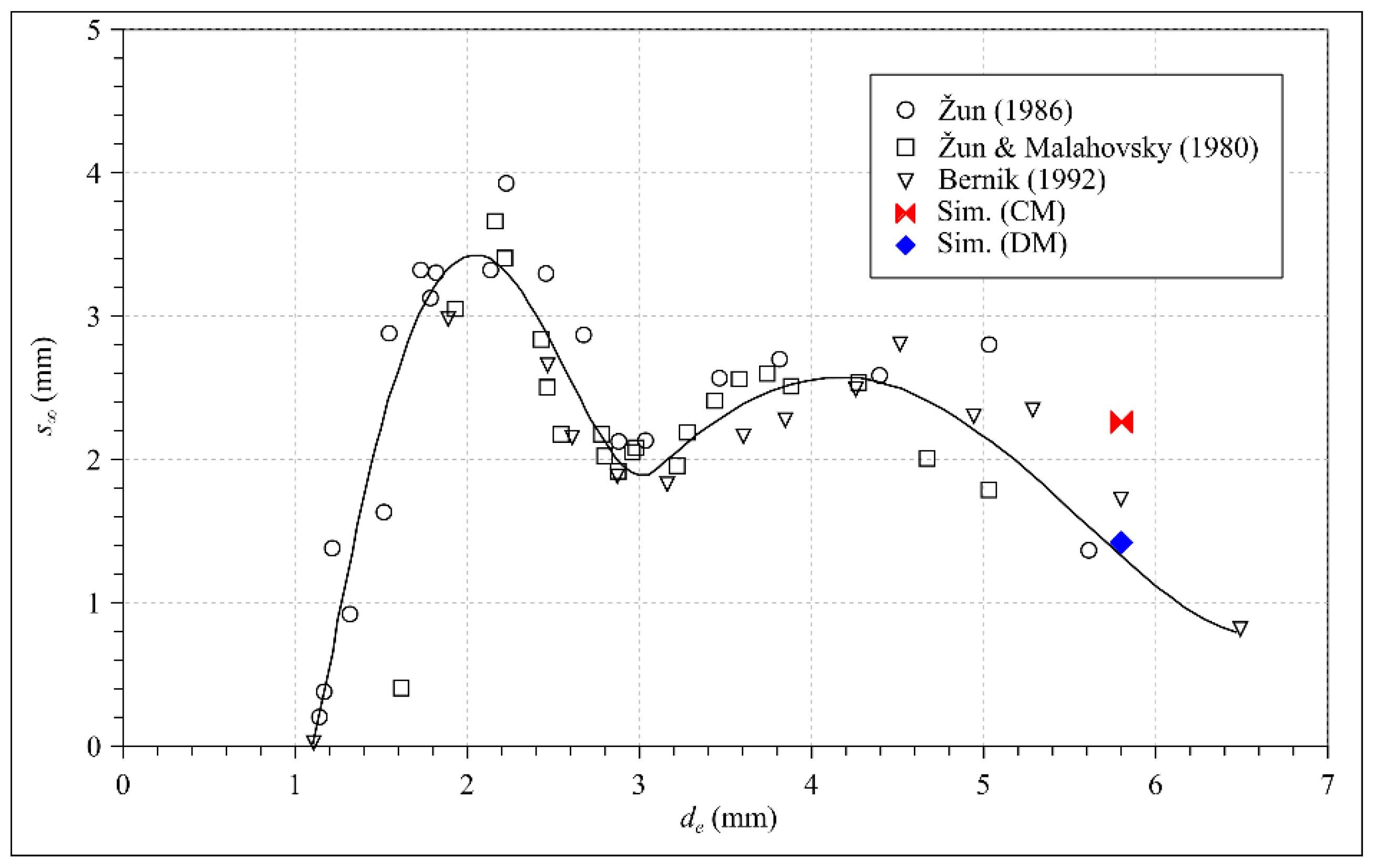
The bubble mean lateral displacement is defined by:
where sj is the bubble center deviation from initial position:
where tj is the time and N is the number of saved time steps. The bubble mean lateral displacement is s∞ = 2.26 mm in the case of a constant mesh and s∞ = 1.42 in the case of a dynamic mesh. The comparison of these two values with the experiment [25] is shown in Figure 5. As we can see, the dynamic mesh value is closer to the measured trend-line than the constant mesh result.
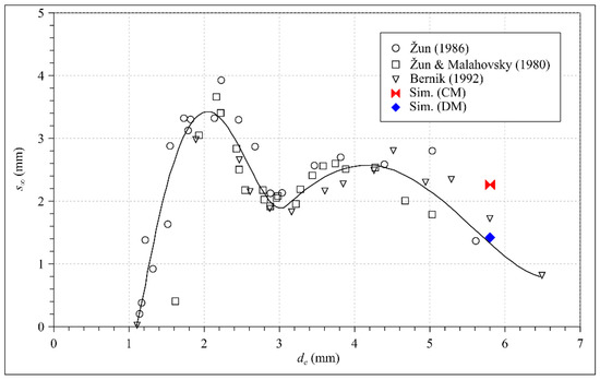
Figure 5.
Bubble mean lateral displacement.
The bubble terminal rise speed is defined by:
For a constant mesh, the bubble terminal velocity is v∞ = 22.56 cm/s and for a dynamic mesh, this is v∞ = 22.59 cm/s. Both values match well with the experimental data (Figure 6).
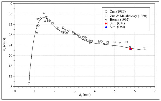
Figure 6.
Bubble terminal rise speed.
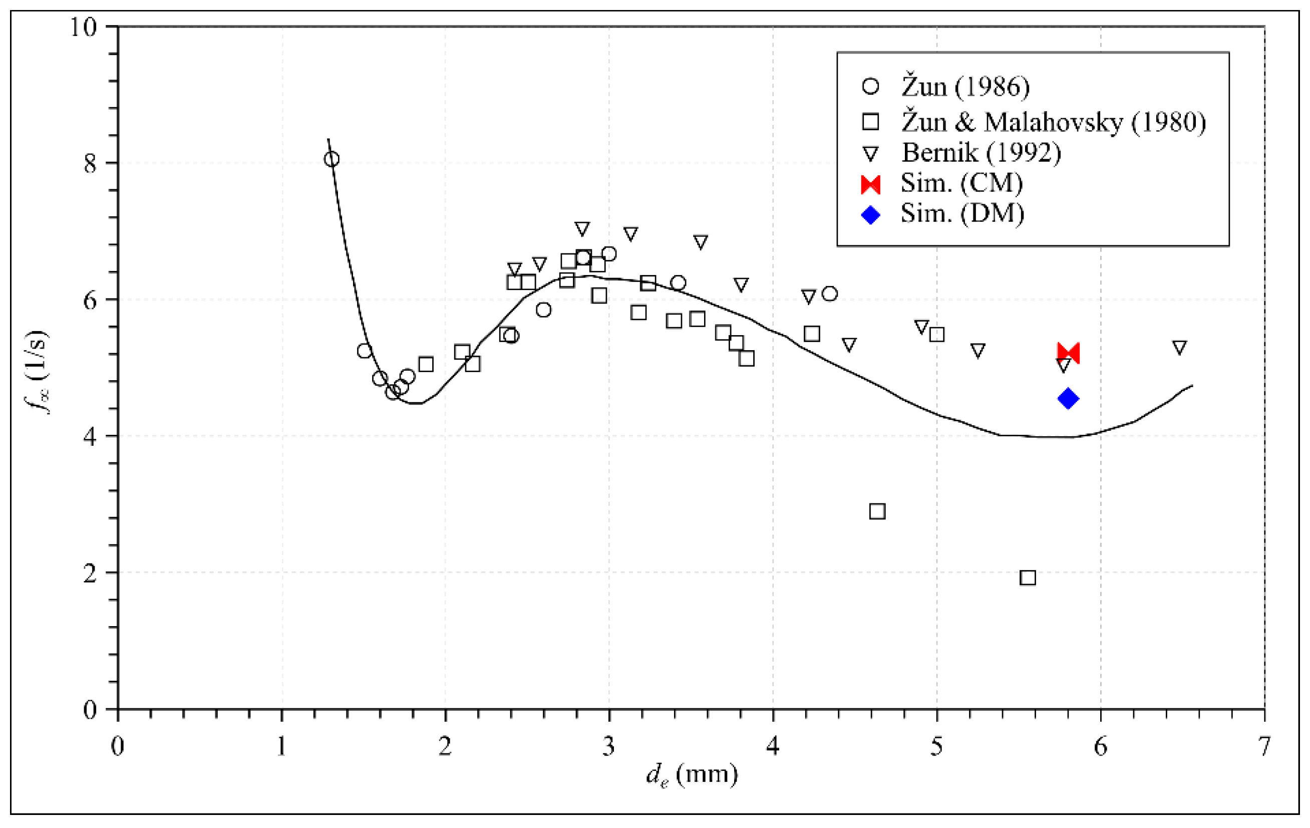
By using the Fast Fourier Transformation (FFT) for the time series of the bubble center coordinates, we calculate the mean oscillation frequency in the bubble wobbling motion. The result is f∞ = 5.21 Hz for a constant mesh and f∞ = 4.55 Hz for a dynamic mesh. The latter value is closer to the measured trend line (Figure 7).
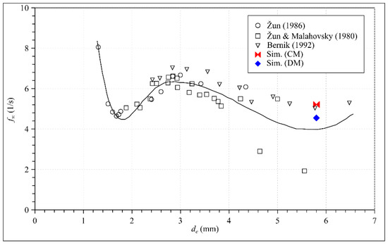
Figure 7.
Mean oscillation frequency in bubble motion.
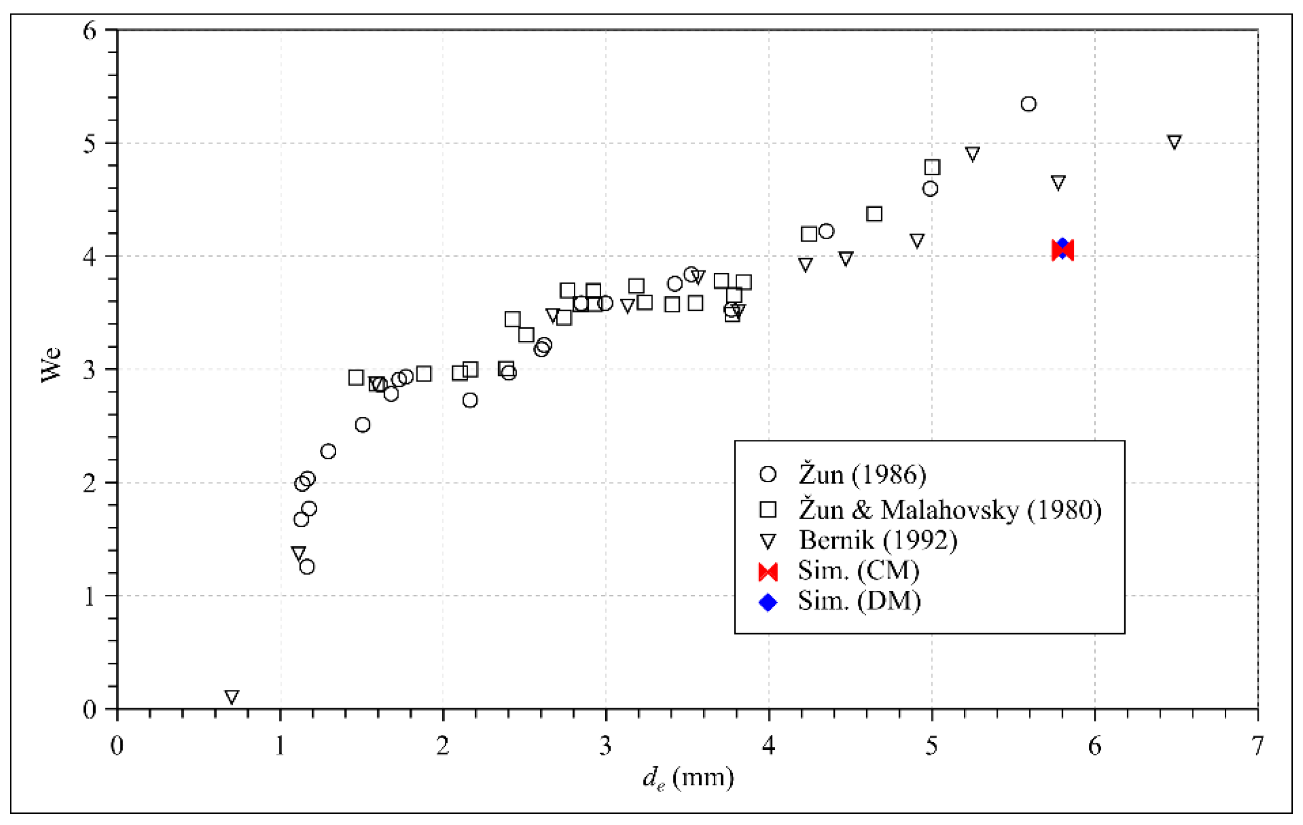
The non-dimensional Weber number represents the ratio of inertial force and surface tension force. The dependence of the Weber number on the bubble equivalent sphere diameter is shown in Figure 8. For the bubble with de = 5.8 mm, the calculated value for a constant mesh is We = 4.05 and We = 4.07 for a dynamic mesh. Both values are slightly lower than the measured ones. This means that the contribution of the inertial force is lower than the actual one in the numerical simulation.

Figure 8.
Weber number vs. bubble equivalent sphere diameter.
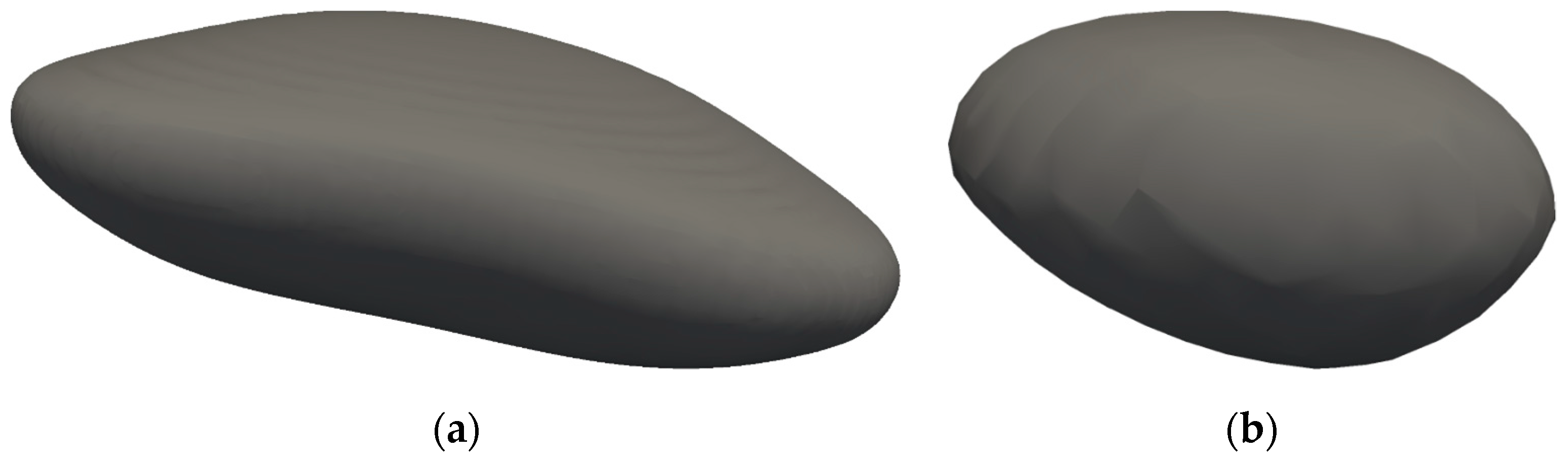
The spherical bubble equivalent diameter = 5.8 mm, where VB is the volume of the bubble, is calculated using the Gauss’s theorem for closed iso-surface α = 0.5, which represents the gas–liquid interface. The free-rising bubble mode can be determined with the help of Grace’s diagram [26], which connects the bubble Eötvos (Eo), Reynolds (Re) and Morton (Mo) dimensionless numbers:
According to the Grace’s diagram, the bubble from the present case is in the wobbling mode. Figure 9 shows the bubble shape at the time t = 1 s. It is in the region of the wobbling mode (time changing) shape with dynamic mesh, while it is closer to ellipsoidal mode shape with constant mesh.
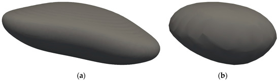
Figure 9.
Bubble shape: (a) Dynamic mesh; (b) constant mesh.
5. Conclusions
The numerical simulation of the free-rising air bubble in a stationary water column was performed by using the open source CFD toolbox OpenFOAM. The constant and dynamic computational meshes were used and the results of the calculation were compared with the experimental data. The interFoam solver was used for the case with time-constant mesh and the interDymFoam for the case with time-varying mesh.
A bigger difference between the calculations is evident in the bubble trajectory. In the case of a constant mesh, the deviation amplitude of the helical path is much smaller than in the case of a dynamic mesh due to a poorer description of the gas–liquid interface.
The bubble terminal velocity and the average frequency of oscillation of the bubble movement fits well with the experimental regression curve in both cases, but the matching is slightly better with the dynamic mesh. The Weber numbers partially deviate from the measured value. The wobbling bubble flow regime, which is obtained by the dynamic mesh, closely matches the Grace’s diagram, while the bubble shape is closer to the ellipsoidal flow regime in the case of the constant mesh.
From the above-mentioned points, we can conclude that the VOF method is suitable for describing and analyzing the two-phase flow with large (according to the size of the computational cells) bubbles. A more detailed description of the gas–liquid interface is obtained by using a dynamic computational mesh, but we must be aware that this means a significant increase in computing time.
Funding
This research was funded by Slovenian Ministry of Education, Science and Sport (grant number P2-0162).
Conflicts of Interest
The authors declare no conflict of interest.
References
- Bombač, A.; Žun, I. Individual impeller flooding in aerated vessel stirred by multiple-Rushton impellers. Chem. Eng. J. 2006, 116, 85–95. [Google Scholar] [CrossRef]
- Hibiki, T.; Ishii, M. Interfacial area concentration in steady fully-developed bubbly flow. Int. J. Heat Mass Transf. 2001, 44, 3443–3461. [Google Scholar] [CrossRef]
- Fletcher, D.F.; McClure, D.D.; Kavanagh, J.M.; Barton, G.W. CFD simulation of industrial bubble columns: Numerical challenges and model validation successes. Appl. Math. Model. 2017, 44, 25–42. [Google Scholar] [CrossRef]
- Talvy, S.; Cockx, A.; Line, A. Modeling of oxygen mass transfer in a gas-liquid airlift, reactor. AIChE J. 2007, 53, 316–326. [Google Scholar] [CrossRef]
- Zun, I.; Perpar, M.; Gregorc, J.; Hayashi, K.; Tomiyama, A. Mixing of thermally stratified water layer by a free rising wobbling air bubble. Chem. Eng. Sci. 2012, 72, 155–171. [Google Scholar] [CrossRef]
- O’Reilly Meehan, R.; Donnelly, B.; Nolan, K.; Persoons, T.; Murray, D.B. Flow structures and dynamics in the wakes of sliding bubbles. Int. J. Multiph. Flow 2016, 84, 145–154. [Google Scholar] [CrossRef]
- Ohta, M.; Imura, T.; Yoshida, Y.; Sussman, M. A computational study of the effect of initial bubble conditions on the motion of a gas bubble rising in viscous liquids. Int. J. Multiph. Flow 2005, 31, 223–237. [Google Scholar] [CrossRef]
- Cano-Lozano, J.C.; Bolaños-Jiménez, R.; Gutiérrez-Montes, C.; Martínez-Bazán, C. The use of Volume of Fluid technique to analyze multiphase flows: Specific case of bubble rising in still liquids. Appl. Math. Model. 2015, 39, 3290–3305. [Google Scholar] [CrossRef]
- Gaudlitz, D.; Adams, N.A. Numerical investigation of rising bubble wake and shape variations. Phys. Fluids 2009, 21, 122102. [Google Scholar] [CrossRef]
- Floryan, J.M.; Rasmussen, H. Numerical Methods for Viscous Flows With Moving Boundaries. Appl. Mech. Rev. 1989, 42, 323–341. [Google Scholar] [CrossRef]
- Osher, S.; Fedkiw, R.P. Level Set Methods: An Overview and Some Recent Results. J. Comput. Phys. 2001, 502, 463–502. [Google Scholar] [CrossRef]
- Sussman, M.; Smereka, P.; Osher, S. A Level Set Approach for Computing Solutions to Incompressible Two-Phase Flow. J. Comput. Phys. 1994, 114, 146–159. [Google Scholar] [CrossRef]
- Hirt, C.W.; Nichols, B.D. Volume of fluid (VOF) method for the dynamics of free boundaries. J. Comput. Phys. 1981, 39, 201–255. [Google Scholar] [CrossRef]
- Rider, W.J.; Kothe, D.B. Reconstructing Volume Tracking. J. Comput. Phys. 1998, 141, 112–152. [Google Scholar] [CrossRef] [Green Version]
- Tomiyama, A.; Shimada, N. A Numerical Method for Bubbly Flow Simulation Based on a Multi-Fluid Model. J. Press. Vessel Technol. 2001, 23, 510–516. [Google Scholar] [CrossRef]
- Besagni, G.; Di Pasquali, A.; Gallazzini, L.; Gottardi, E.; Colombo, L.P.M.; Inzoli, F. The effect of aspect ratio in counter-current gas-liquid bubble columns: Experimental results and gas holdup correlations. Int. J. Multiph. Flow 2017, 94, 53–78. [Google Scholar] [CrossRef]
- Fuster, D.; Agbaglah, G.; Josserand, C.; Popinet, S.; Zaleski, S. Numerical simulation of droplets, bubbles and waves: State of the art. Fluid Dyn. Res. 2009, 41, 065001. [Google Scholar] [CrossRef]
- Brackbil, J.; Kothe, D.B.; Zemach, C. A continuum method for modeling surface tension. J. Comput. Phys. 1992, 100, 335–354. [Google Scholar] [CrossRef]
- OpenFOAM. The Open Source CFD Toolbox: User Guide; OpenFOAM Foundation: London, UK, 2014. [Google Scholar]
- Marić, T.; Höpken, J.; Mooney, K. The OpenFOAM Technology Primer; Sourceflux: Duisburg, Germany, 2014. [Google Scholar]
- Rek, Z.; Gregorc, J.; Bouaifi, M.; Daniel, C. Numerical simulation of gas jet in liquid crossflow with high mean jet to crossflow velocity ratio. Chem. Eng. Sci. 2017, 172, 667–676. [Google Scholar] [CrossRef]
- Tomiyama, A. Some Attempts for the Improvement of Computational Bubble Dynamics. In Proceedings of the 10th Workshop on Two-Phase Flow Predictions, Merseburg, Germany, 9–12 April 2002; pp. 125–136. [Google Scholar]
- OpenFOAM. The OpenSource CFD Toolbox: Programmer’s Guide; OpenFOAM Foundation: London, UK, 2014. [Google Scholar]
- Fric, T.F.; Roshko, A. Vortical structure in the wake of a transverse jet. J. Fluid Mech. 1994, 279, 1–47. [Google Scholar] [CrossRef]
- Zun, I.; Groselj, J. The structure of bubble non-equilibrium movement in free-rise and agitated-rise conditions. Nucl. Eng. Des. 1996, 163, 99–115. [Google Scholar] [CrossRef]
- Clift, R.; Grace, J.R.; Weber, M.E.; Weber, M.F. Bubbles, Drops and Particles; Academic Press: Cambridge, MA, USA, 1978; ISBN1 012176950X. ISBN2 9780121769505. [Google Scholar]


© 2019 by the author. Licensee MDPI, Basel, Switzerland. This article is an open access article distributed under the terms and conditions of the Creative Commons Attribution (CC BY) license (http://creativecommons.org/licenses/by/4.0/).