Steady Two-Dimensional Free-Surface Flow Past Disturbances in an Open Channel: Solutions of the Korteweg–De Vries Equation and Analysis of the Weakly Nonlinear Phase Space

Abstract

Two-dimensional free-surface flow past disturbances in an open channel is a classical problem in hydrodynamics—a problem that has received considerable attention over the last two centuries (e.g., see Lamb’s Treatise, 1879). With traces back to Russell’s experimental observations of the Great Wave of Translation in 1834, Korteweg and de Vries (1895), and others, derived an unforced equation to describe the balance between nonlinearity and dispersion required to model the solitary wave. More recently, Akylas (1984) derived a forced KdV equation to model a pressure distribution on the free-surface (e.g., a ship). Since then, the forced KdV equation has been shown to be a useful model approximation for two-dimensional flow past disturbances in an open channel. In this paper, we review the stationary solutions of the forced KdV equation for four types of localised disturbances: (i) a flat plate separating two free surfaces; (ii) a compact bump, or dip in the channel bottom topography; (iii) a compact distribution of pressure on the free surface and (iv) a step-wise change in the otherwise constant horizontal level of the channel bottom topography. Moreover, Dias and Vanden-Broeck (2002) developed a phase plane method to analyse flow over a bump, and this general approach has also been applied to the three other types of forcing (see Binder et al., 2005–2015, and others). In this study, we use eleven basic flow types to classify the steady solutions of the forced KdV equation using the phase plane method. Additionally, considering solutions that are wave-free both far upstream and far downstream, we compare KdV model approximations of the uniform flow conditions in the far-field with exact solutions of the full problem. In particular, we derive a new KdV model approximation for the upstream dimensionless flow-rate which is conveniently given in terms of the known downstream dimensionless flow-rate.

1. Introduction

It is understood that free-surface flow occurs over channel beds within tidal estuaries, streams, irrigation channels, rivers and hydraulic infrastructures [1,2,3,4,5,6], and that when the speed of the base flow is close to the critical speed $\sqrt{gH}$, where H is the depth of the channel, surface waves generated by disturbances in a channel can damage both the integrity of waterway banks and hydraulic infrastructures. The study of free-surface flow has also explored energy lost in surface waves as an important component of the overall drag on the disturbance (e.g., the steady wave pattern and drag at the stern of a ship) [7,8,9,10,11,12,13]. The nature of research into free-surface flow has led to experimental studies predominantly in rectangular open channels [14,15,16,17,18,19] (e.g., see Figure 1). Understanding the fundamentals of such flows has been important in applications where there is a desire to protect waterway banks and hydraulic infrastructures, and reduce the wave-drag on a moving disturbance.

The study of steady two-dimensional flow in a finite depth channel has been a classical problem in hydrodynamics with a rich and long history [8,9,20,21,22,23,24,25,26]. More recently, the flow problem has continued to attract attention through both the computation of numerical solutions to the full problem and analysis of the weakly nonlinear problem [27,28,29,30,31,32,33,34,35,36]. The primary purpose of this paper is to review the relatively recent advances made in this field of research through the examination of the steady solution space in the weakly nonlinear phase plane of the problem. We begin by considering the potential free-surface flow past disturbances in an open channel, as shown in Figure 2. The fluid-flow in the channel is perturbed by four types of disturbances. The first is a flat plate that separates two portions of the free surface, such as a sluice gate, or surfboard [28,37,38,39,40,41,42,43]. The second is a compact bump, or dip in the topography [8,20,23,26,34,35,44,45]. The third is a compact distribution of pressure on the free-surface, which may model the normal stress on the free-surface generated by a moving ship [36,46,47,48,49], or the Maxwell stress due to a charged electrode [50]. The fourth is a rapid change, or step from one horizontal flat level in the topography to another horizontal flat level [51,52,53,54,55,56]. In addition, hybrid problems are also examined in which a combination of the four types of disturbances is considered [33,50,57,58,59].

The location of the free surface is given by $y^{*}=H+{\eta }^{*}(x^{*})$, where ${\eta }^{*}$ is the elevation of the free surface, and the channel bottom topography and distribution of pressure on the free-surface are denoted by ${\sigma }^{*}(x^{*})$ and $p^{*}(x^{*})$, respectively. It is assumed that there is uniform flow far downstream where the flow approaches a uniform stream with constant velocity U and depth H, and therefore ${\eta }^{*}(x^{*})\to 0$, $p^{*}(x^{*})\to 0$ and ${\sigma }^{*}(x^{*})\to 0$ as $x^{*}\to \infty$. A sketch of a typical flow configuration is shown in Figure 2. With these conditions, the flow can be characterised by the dimensionless flow rate, or downstream depth-based Froude number

$$F=\frac{U}{\sqrt{gH}},$$

(1)

where g is the acceleration due to gravity. When $F<1$, the flow far downstream is called subcritical and for $F>1$ the flow far downstream is called supercritical. The terms subcritical and supercritical come from linear theory, which predicts that supercritical flows are waveless [20]. This can be seen by examining the linear dispersion relation [20], and it shows that the speed, $c=\sqrt{gH}$, of small-amplitude waves in shallow water is non-dispersive, because c is independent of the wavenumber, or wavelength. The Froude number, therefore, represents the ratio of the uniform flow speed to the speed of small-amplitude (non-dispersive) waves in shallow water. When the flow is also uniform far upstream, as $x^{*}\to -\infty$, with constant velocity V and constant depth D, an additional upstream Froude number is defined by

$$F_u=\frac{V}{{(gD)}^{1/2}}.$$

(2)

The solutions to the steady two-dimensional flow problem can be classified using the Froude number, F, and the features of the flow far upstream as $x^{*}\to -\infty$. There are eleven basic steady flow types [60]:

I

Supercritical flow with $F=F_u>1$ [24,26,49]

II

Critical flow with $F=F_u=1$ [45,60,61]

III

Subcritical flow with $F<1$ and waves as $x^{*}\to -\infty$ [8,9,50]

IV

Generalised hydraulic fall with $F>1$ and waves as $x^{*}\to -\infty$ [27,28,30]

V

Hydraulic fall with $F>1$ and $F_u<1$ (or $F_u<1$ and $F>1$) [23,26,59]

VI

Supercritical flow with $F>1$ and $F_u>1$, with $F\ne F_u$ [33,54,60]

VII

Subcritical flow with $F=F_u<1$ [8,56,57]

VIII

Subcritical flow with $F<1$ and $F_u<1$, with $F\ne F_u$ [44,60]

IX

Critical flow with $F=1$ and waves as $x^{*}\to -\infty$ [33,54,60]

X

Critical flow with $F=1$ and $F_u>1$ [33,60]

XI

Critical flow with $F=1$ and $F_u<1$ [33,60].

Note that the steady two-dimensional potential flow approximation implies that the direction of the flow may be reversed [7,30,50,57]. This is pertinent to the interpretation of flow types III and IV in which there are waves far upstream. These two flow types apparently violate the radiation condition [22], which requires that the waves are generated by the disturbances, but since the flow is reversible, the direction of the flow may be viewed instead as being from right to left, thus satisfying the radiation condition. The reversibility of the flow also applies to the other nine flow types and, for example, when the direction of flow is reversed in flow type V it is referred to as hydraulic rise instead of a hydraulic fall. As we shall see later, the reversibility of flow can be explained with reference to an analysis in the weakly nonlinear phase plane of the problem.

Although solutions to flow types I–XI in the full problem may be investigated by careful numerical experimentation, it has been shown to be advantageous to examine the flow types in the weakly nonlinear phase plane of the problem [27,28,54,62]. This approach has been shown to be useful in determining the different types of possible solutions, and the number of independent parameters and their approximate values which can be used as initial guesses in numerical computations of solutions to the full problem [27,28,45,54,61]. Many new flow types have been discovered by performing an analysis in the weakly nonlinear phase plane of the flow problem, and the forced Korteweg–de Vries (fKdV) equation is often used to model the weakly nonlinear flow problem.

In the weakly nonlinear problem, the different types of possible solutions for a given type of disturbance can be established by examining the permissible movements between the fixed points and trajectories in the phase plane. The four types of disturbances (plate, compact topography and pressure distribution, step up/down in topography) produce three different types of permissible movements: (i) a flat plate gives a horizontal jump [28,62]; (ii) a compact topographical disturbance or pressure on the free-surface gives a vertical jump [27,62]; and (iii) a step change in the level of an otherwise flat and horizontal channel topography gives the intersection between equilibria and trajectories of two phase planes [54]. Solutions to hybrid flows, in which there is a combination of the four types of disturbances in the channel (see Figure 2), can also be obtained by examining a combination of the three types of permissible movements in the phase plane [33,50,57,58,59].

In addition to reviewing the phase plane analysis, the equilibria in the weakly nonlinear problem that are associated with uniform flow (e.g., uniform flow both far upstream and far downstream as seen in Figure 2, points A and B), can also be compared to exact solutions of the full problem, and therefore provide a way to ascertain the range of validity of the weakly nonlinear analysis for solutions that are waveless in the far-field [28,54]. These wave-free flow-types I, II, V, VI, VII, VIII, X, XI may have application to the design of hydraulic infrastructures and ship-hulls, in which it is often desirable to reduce surface waves, and an important quantity of interest is the upstream Froude number, $F_u$. Using a simple transformation of the weakly nonlinear free-surface elevation and its associated equilibria [63], we derive a new formula to approximate the value of the upstream Froude number. This new, simple formula may be of practical importance as it provides the means to quantify the upstream flow conditions without recourse to the more complicated expressions and numerical computations of solutions to the full problem.

2. Methods

This paper considers the steady two–dimensional irrotational flow of an incompressible inviscid fluid bounded by the free surface (and plate if present) and topography. Dimensionless quantities can be made by taking the uniform velocity U as the velocity scale and uniform depth H as the length scale. The governing equation within the fluid is Laplace’s equation for the velocity potential, $\varphi$. The flow must also satisfy the uniform flow conditions far downstream, the kinematic boundary conditions on both the free-surface (and plate if present) and topography, and the dynamic boundary condition on the free-surface. The latter of these conditions is what makes the full problem difficult to solve because it is a nonlinear and unknown boundary condition which is found as a part of the solution. This defines the potential flow model for the full problem, and fully nonlinear solutions can be computed using boundary integral methods [8,19,26,43,45,49,60,64].

As stated in the Introduction, the determination of the number of independent parameters needed to obtain a unique solution to a free-surface problem is often delicate and counter intuitive. It can be found by careful numerical experimentation, however an alternative method of solution is to perform an analysis in the weakly nonlinear phase plane [27,28,54] of the problem. This approach allows for a systematic determination of all the possible solutions, when within the range of validity of the weakly nonlinear analysis.

In this study, we review the weakly nonlinear phase plane analysis of the fKdV model equation. The first derivation of the unsteady fKdV equation was for forcing given by a distribution of pressure, $p(x)$, on the free-surface [46,65], and the same equation can be derived for a topographical disturbance, $\sigma (x)$,25,66,67,68]. It is important to note that there are two regimes where the weakly nonlinear theory may not be applicable. The first of these is when the waves are very steep and are approaching the Stokes limiting configuration of an included angle of 120° at the wave crest(s) [49,69]. The second regime is when the flow is intrinsically unsteady, and is often referred to as transcritical flow [25,32,34,52,55,61,70], which is characterised by solitons being periodically emitted upstream of the disturbance with a uniform depression and wake downstream (e.g., see the waterfall plots in Figure 6 [34,49,71]). However, when within the range of validity of the weakly nonlinear theory, analysis in the phase plane of the problem provides a systematic way to classify the different types of solutions.

When written in terms of the dimensionless variables, the unsteady fKdV equation takes the form

$$\begin{array}{cc}\hfill 6{\eta }_t+{\eta }_{xxx}+9\eta {\eta }_x-6(F-1){\eta }_x& =-3f_x\hfill \end{array}$$

(3)

where f represents the forcing due to either a distribution of pressure on the free surface, p, a topographical disturbance, $\sigma$, or a linear combination of both types of disturbances (e.g., a hybrid flow with $f=p+\sigma$). The fKdV equation is an asymptotic approximation to the full problem. Its derivation is based on long wavelength asymptotics, which we briefly discuss here. A small parameter $ϵ={(H/L)}^2\ll 1$ is introduced along with the dimensionless quantities $(x^{\prime },y^{\prime })=({ϵ}^{1/2}{x}^{*},y^{*})/H$, $t^{\prime }={ϵ}^{3/2}{t}^{*}$, ${\eta }^{\prime }={ϵ}^{-1}{\eta }^{*}/H$ and $f^{\prime }={ϵ}^{-2}{f}^{*}/H$, where L denotes a typical horizontal length scale. Substituting expansions in powers of $ϵ$ into the potential equations (rewritten in terms of the scaled variables), the fKdV equation is derived by equating coefficients of the powers of $ϵ$. For example, the expansion for the Froude number is $F=1+ϵF_1+\cdots$. When written in terms of dimensionless variables, x, $\eta$ and f, the fKdV equation takes the form of Equation (3) (see [27,46] and others). The case of when there is a plate separating two portions of the free-surface will be discussed in Section 3.2.

Note that the second and third terms in the left-hand side of Equation (3) represent the effect of dispersion and nonlinearity in the problem. In addition, linearization of Equation (3) and setting the forcing term to zero yields a cubic dispersion relation for linear sinusoidal waves (i.e., $\eta =acos(kx-wt)$) of frequency $\omega$ and wavenumber k. This (linear) dispersion relation illustrates that waves of different wavenumbers and therefore different wavelengths disperse at different speeds, $c=\omega /k$, which is not predicted by the linear theory of waves in shallow water. Asymptotic approximations for nonlinear dispersion relations can be derived by substituting Stokes expansions into the equations that describe the full problem (and the unforced KdV equation) which are solved at successive orders of the approximation [72]. Typically, the wave speed does not only depend on the wavelength, but also on the wave amplitude in nonlinear dispersion relations.

If the flow is steady, Equation (3) can be integrated to obtain

$$\begin{array}{ccc}\hfill {\eta }_{xx}+\frac{9}{2}{\eta }^2-6(F-1)\eta & =& -3f,\hfill \end{array}$$

(4)

where the boundary conditions for uniform flow far downstream

$$\begin{array}{c}\hfill \eta \to 0{\eta }_x\to 0{\eta }_{xx}\to 0\mathrm{and}f\to 0\mathrm{as}x\to \infty ,\end{array}$$

(5)

have been used to evaluate the constant of integration.

The objective now is to examine the solutions of Equation (4) that satisfy the boundary conditions Equation (5). Where applicable, the numerical solutions of Equation (4) presented in this work have been reproduced using the numerical methods referenced in the figure captions.

3. Results

The results are organised as follows. To begin with, we discuss the case of the unforced problem in Section 3.1, where there is no plate and $f=0$ in Equation (4). In Section 3.2, the first of the disturbances, a flat plate that separates two portions of the free surface, is studied. As we have already discussed, the forcing due to either a compact topographic disturbance or compact distribution of pressure on the free-surface have the same model equation. Therefore, the analysis for both of these types of disturbances is presented in Section 3.3. The fourth type of disturbance, a step in the topography, is examined in Section 3.4. Hybrid flows are considered in Section 3.5.

3.1. Unforced Flow with No Disturbances

When there is no forcing, $f=0$. Therefore, Equation (4) is autonomous and it can be re-written in the form of a two-dimensional nonlinear dynamical system [27,61,62,73,74,75] with the following equilibria

$${\eta }_{\pm }=\frac{2}{3}(F-1)\pm \frac{2}{3}\left|(F-1)\right|\mathrm{and}{\eta }_x=0$$

(6)

in the weakly nonlinear phase plane, $(\eta ,{\eta }_x)$. For $F\ne 1$, the fixed point $({\eta }_{+},0)$ is a centre and the fixed point $({\eta }_{-},0)$ is a saddle, and the location of the two fixed points in the phase plane depends on whether $F>1$ or $F<1$. If $F>1$, there is a saddle at the origin and a centre at $(4/3(F-1),0)$. If $F<1$, there is centre at the origin and a saddle at $(4/3(F-1),0)$. When $F=1$, the two fixed points, $({\eta }_{\pm },0)$, coalesce into a single degenerate node at the origin.

Multiplying Equation (4) by ${\eta }_x$ and integrating yields

$${\eta }_x^2=6(F-1){\eta }^2-3{\eta }^3+C,$$

(7)

where C is a constant of integration. Equation (4) can be used to plot the trajectories or orbits in the phase plane for different values of C as is shown in the phase portraits of Figure 3.

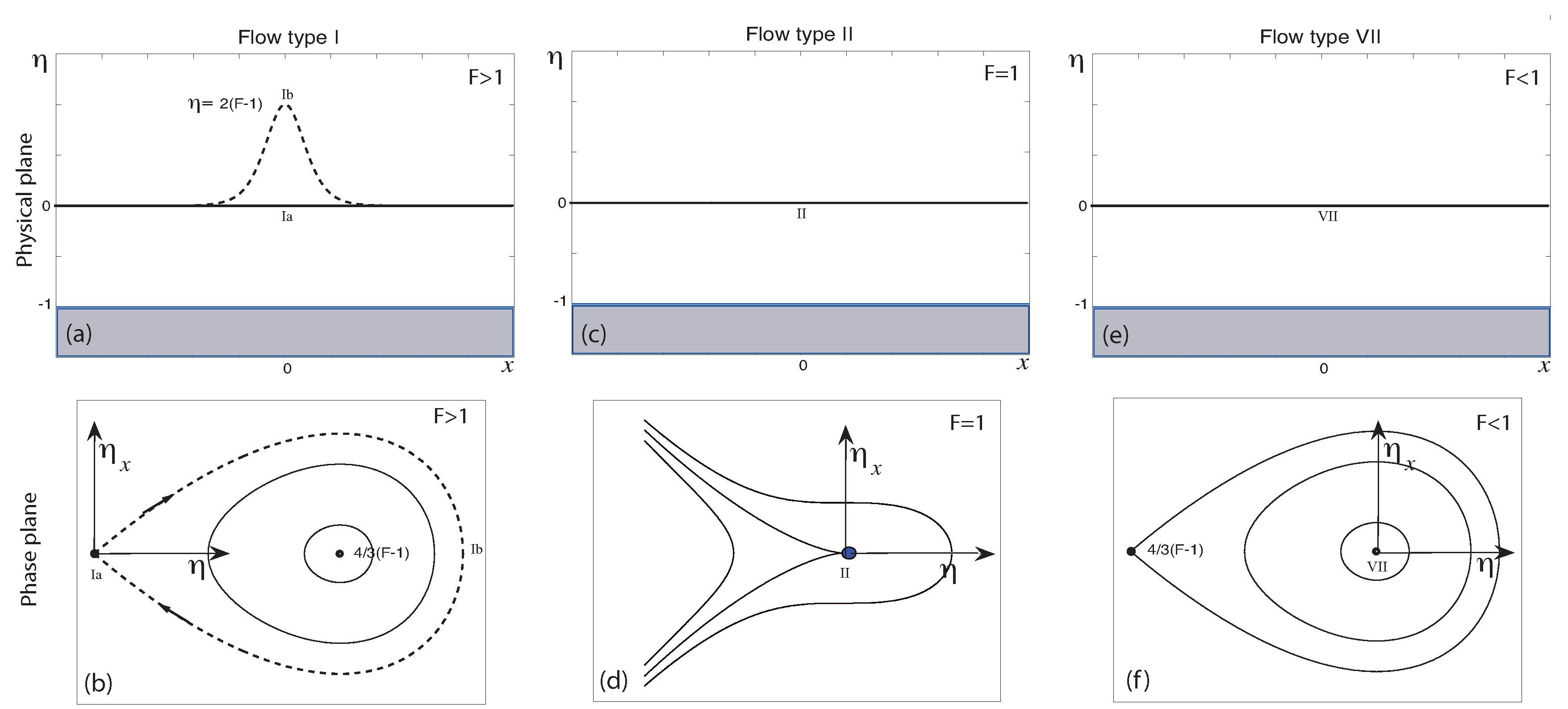
In the case of no forcing, there are three trivial solutions that correspond to uniform flow in the physical plane (solid lines), and in the phase plane these solutions are represented by the three fixed points located at the origin (see Figure 3). However, for supercritical flow with $F>1$ there is an additional nontrivial solution, the well-known unforced solitary wave

$$\eta (x)=2(F-1){sech}^2\left(\sqrt{\frac{3(F-1)}{2}}x\right).$$

(8)

The unforced solitary wave is seen as the homoclinic orbit connecting the saddle at the origin to itself in the phase plane (broken curve for a value of $C=0$ in Figure 3b).

Equation (8) (or Equation (7) with $C=0$ and ${\eta }_x=0$) give the maximum elevation of the unforced solitary wave,

$$\eta (0)=2(F-1),$$

(9)

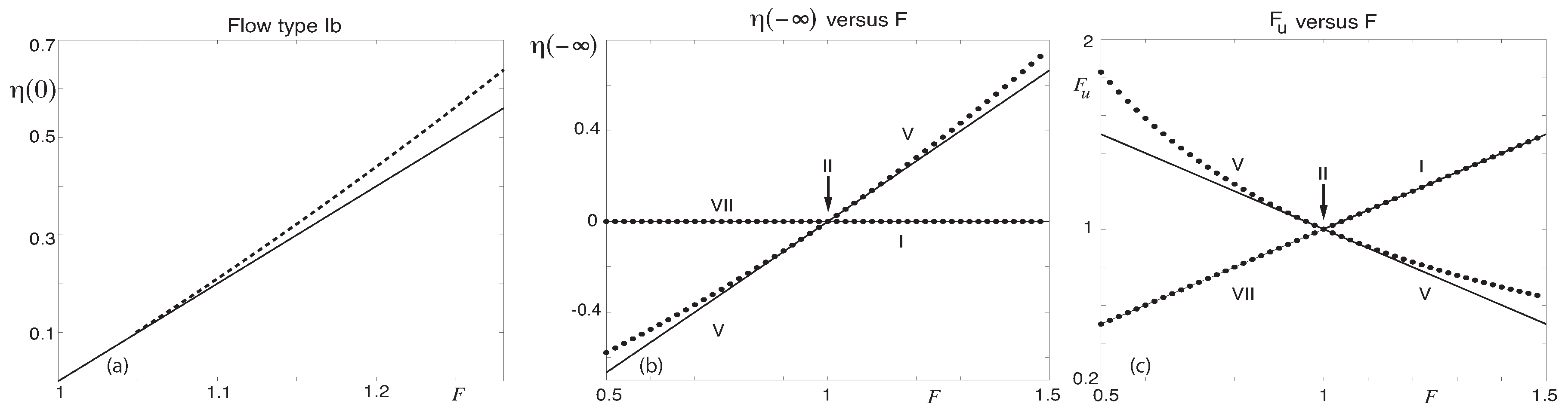
which can be compared to computed numerical values of the maximum elevation of the unforced solitary wave in the full problem. The comparison is presented in Figure 4a where it is seen that there is good agreement between the weakly nonlinear and fully nonlinear results for values of the Froude number $1<F<1.15$, and this provides us with a quantitative measure for the range of validity of the weakly nonlinear analysis for flow type Ib.

It is important to note that the four types of unforced solution come from one parameter families for a given value of F, which satisfy the uniform flow conditions Equation (5) used in the derivation of Equation (4). Furthermore, all solutions, whether unforced or forced, must terminate at the origin in the phase plane in order to satisfy the boundary conditions Equation (5). Therefore, and according to the weakly nonlinear phase plane analysis, there are no other unforced flow types as it impossible to construct solutions in the phase plane that connect (bounded) trajectories with the origin, other than that of the homoclinic orbit in the case of when $F>1$. As we shall see in the proceeding Sections, forced solutions provide a way to move between trajectories and fixed points in the phase plane, allowing for additional types of solutions.

Before we discuss the different types of forced solutions, it is useful to compare exact solutions of the full problem with corresponding values from the weakly nonlinear analysis for waveless uniform flow in the far-field, with ${\eta }_x(\pm \infty )=0$ (and $f(\pm \infty )=0$), without reference to the specific details of the type of disturbance(s) in the channel. The only additional assumption we make at this stage is that the topography has the same horizontal level in the far-field, with $\sigma (\pm \infty )=0$. Without loss of generality, it can be shown [28] (and others) that exact solutions of the full problem must satisfy the relations

$$F^2(1-{(1+\eta (-\infty ))}^2){=2(1-(1+\eta (-\infty ))(1+\eta (-\infty ))}^2$$

(10)

and

$$F_u=F{(1+\eta (-\infty ))}^{-3/2}.$$

(11)

With the aforementioned conditions, and in terms of the weakly nonlinear theory, it is reasonable to assume that the uniform flow in the far-field may be approximated by the autonomous unforced KdV equation. It is now possible to consider (forced) solutions that not only begin and end their journey at the same fixed point in the phase plane (see Figure 3b,d,f, with $F_u=F$ and $\eta (\infty )=\eta (-\infty )=0$), but also solutions that begin and end their journey at two different fixed points in the phase plane (see Figure 3b,f, with $F_u\ne F$, $\eta (\infty )=0$ and $\eta (-\infty )=4/3(F-1)$). All that remains is the derivation of a weakly nonlinear expression for the upstream Froude number in the case of when $F_u\ne F$ and $\eta (-\infty )=4/3(F-1)$. The derivation involves a transformation of the constant-level solution far upstream to the origin [63], which is generalised here.

Consider the transformation $\eta =\widehat{\eta }+S$ in Equation (4) which yields

$$\begin{array}{ccc}\hfill {\eta }_{xx}+\frac{9}{2}{\eta }^2-6((F-1)-\frac{3}{2}S)\eta +\frac{9}{2}{S}^2-6(F-1)S& =& -3f,\hfill \end{array}$$

(12)

after dropping the carets. For the problem in hand, $S=4/3(F-1)$ and Equation (12) reduces to

$$\begin{array}{ccc}\hfill {\eta }_{xx}+\frac{9}{2}{\eta }^2-6(-(F-1))\eta & =& -3f,\hfill \end{array}$$

(13)

with the same conditions given by Equation (5) now being satisfied when $x\to -\infty$. The upstream Froude number can now be expressed in terms of the downstream Froude number by simply examining the coefficient for $\eta$ in Equation (13), and we find that

$$F_u=2-F$$

(14)

in the weakly nonlinear framework. Note that Equation (14) (and Equation (11) in the the full problem) immediately rule out the possibility of solution types VI, VIII, X, XI when $\sigma (\pm \infty )=0$.

The comparison between exact solutions of the full problem, Equations (10) and (11), and values of the weakly nonlinear analysis, Equations (6) and (14), is presented in Figure 4b,c, and illustrate that only four of the eight basic flow types that are wave-free in the far-field are possible with the constraints considered so far. The results also show that there is good quantitative agreement between the two theories when $0.8<F<1.2$ for flow type V. Furthermore, it is important to recognise that the analysis does not guarantee the existence of solutions for a given type of disturbance, or forcing and this needs to be established on a case-by-case basis. The first type of disturbance we consider is that of flow past a plate that separates two portions of the free surface.

3.2. Flow Past a Flat Plate

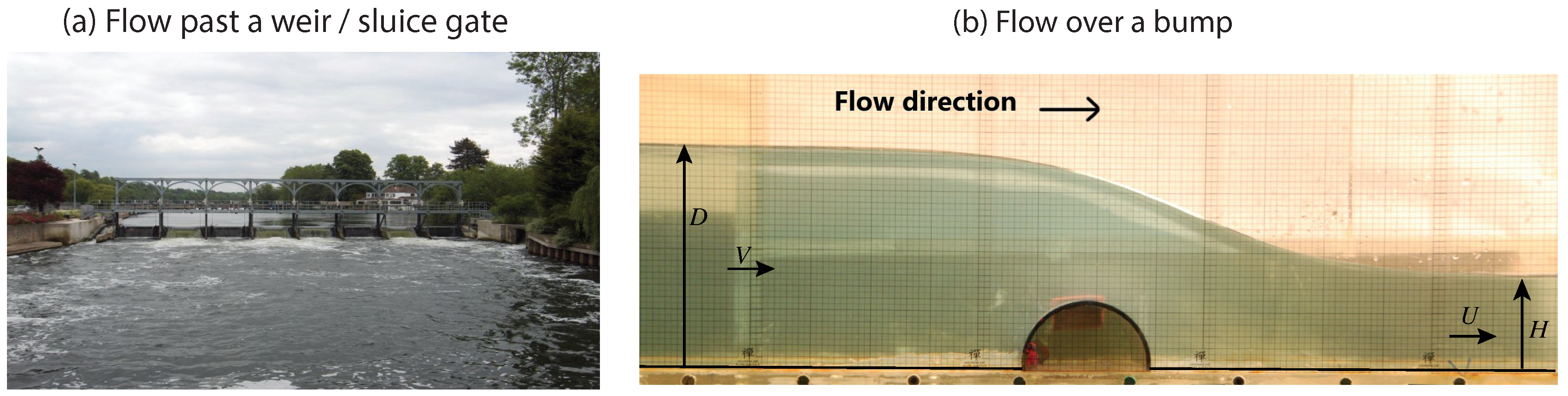
Having examined the unforced problem in the weakly nonlinear phase space, we now consider a flow that is perturbed by a flat plate inclined at an angle $\theta >0$ to the horizontal line that separates two portions of the free surface as is illustrated in Figure 5. Free-surface flow past a plate is a model approximation to flow past a sluice gate, or surfboard [28,37,38,39,40,41,42,43]. In terms of the weakly nonlinear analysis, solutions can be constructed by combining the trajectories associated with Equation (7) (i.e., $f=0$ in Equation (4)) on the free-surface with the known value of

$${\eta }_x=-tan\theta$$

(15)

on the plate. Equation (15) gives a horizontal line, or jump in the phase plane $(\eta ,{\eta }_x)$. The key idea amounts to using the unforced autonomous phase plane diagrams of Figure 3 to model the two portions of the free surface that intersect with the constant slope of the plate, thus providing a way to examine and classify the existence of steady solutions of the potential flow model approximation for flow past a plate. In particular, we show that out of the possible four basic flow types I, II, V, VII that are wave-free in the far-field in the case when $\sigma (\pm \infty )=0$, only the supercritical flow type I exists [28].

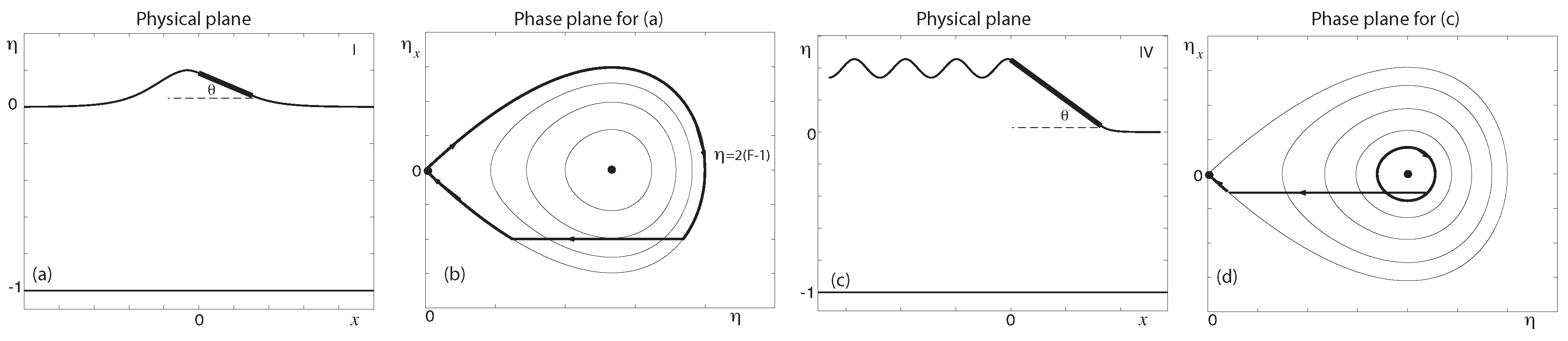
For the supercritical flow type I, we now analyse the weakly nonlinear phase plane of Figure 5b to determine the number of independent parameters in the corresponding weakly nonlinear profile Figure 5a. For a given value of $F>1$, we can plot the phase plane shown in Figure 5b. Then, a given value of $\theta >0$ determines the horizontal line in the phase plane Figure 5b. In the case of flow type I, we have already seen that a solution trajectory in the phase plane must begin and end its journey at the saddle point in order to satisfy the constraints $\eta ={\eta }_x=0$ as $x\to \pm \infty$, with $F=F_u>1$. Therefore, we start to move from the saddle point at the origin, in a clockwise direction on the solitary wave orbit, $C=0$, past the maximum elevation $\eta =2(F-1)$, ${\eta }_x=0$. At the intersection of the upstream portion of the free-surface with plate, there is a horizontal jump, given by Equation (15), to the intersection of the downstream portion of the free-surface with the plate, before returning to the saddle point via the solitary wave orbit. The analysis in the phase plane suggests that there is a two parameter family of solutions for given values of $F>1$ and $\theta >0$, which has been confirmed in both the weakly nonlinear (see Figure 5a) and the full problem [28,41], with the length of the plate, L, coming as a part of the solution.

The intersections of the plate with the upstream and downstream free surfaces can be determined as follows. Using Equations (15) and (7), with $C=0$, we obtain a cubic for $\eta$

$$6(F-1){\eta }^2-3{\eta }^3={tan}^2\theta ,$$

(16)

and define the three roots as ${\eta }_3<{\eta }_2<{\eta }_1$. The first and second roots, ${\eta }_1$ and ${\eta }_2$, are then the elevation of the plate at the intersection with upstream and downstream portions of free surface, respectively. We note that the third root, ${\eta }_3<0$, is of no interest to us as it corresponds to the intersection of the horizontal line with the unbounded trajectory emanating from the origin into the third quadrant of the phase plane, $\eta <0$ and ${\eta }_x<0$, leading to an unbounded solution (see, for example, the unbounded trajectories in the phase planes for supercritical flow in Figure 6). The length of the plate,

$$L=({\eta }_1-{\eta }_2)/sin\theta ,$$

(17)

must then come as part of the solution, to ensure that the phase trajectory leaves and rejoins the solitary wave orbit in the phase plane Figure 5b. Notice that when $L\to 0$, we obtain the maximum value of

$$\theta =arctan(\frac{4\sqrt{2}}{3}{(F-1)}^{3/2}),$$

(18)

from Equation (16) with $\eta =\frac{4}{3}(F-1)$, and recover the unforced solitary wave solution. Therefore, the solution can be classified as a perturbation of a solitary wave. Consistent with our previous analysis for the unforced solitary wave as shown in Figure 4a, there is good quantitative agreement between the weakly nonlinear and the fully nonlinear results for $1<F<1.15$ [28,41]. In contrast, if we consider the case when $\theta \to 0$, then $L\to \infty$, ${\eta }_1\to 2(F-1)$, ${\eta }_2\to 0$, and we obtain a solution for supercritical past a semi-infinite flat horizontal plate [28] (and others).

The only other solution for flow past a flat plate of finite length with $\theta \ne 0$ that satisfies the boundary conditions Equation (5) is the basic generalised hydraulic fall flow type IV [28], with $F>1$ and a train of waves on the free surface as $x\to -\infty$. The number of independent parameters is three, and they can be determined by examining the phase plane diagram of Figure 5d. Similar to our previous analysis for flow type I, given values of $F>1$ and $\theta >0$ determine the general features of the phase portrait and the horizontal line in the phase plane. The additional, third independent parameter can now be chosen as the length of the plate, $L>0$, and this determines the amplitude of the waves on the upstream free surface in Figure 5c, which are seen as the inner periodic orbits in Figure 5d. It is worth mentioning that for given values of F and $\theta$ there are two types of solution, corresponding to two different values of L, with waves on the upstream free-surface that have the same amplitude. One of these solutions is shown in Figure 5c,d where the elevation of the plate at the intersection of the upstream free surface is to the right of the centre, ${\eta }_1>\frac{4}{3}(F-1)$. The second solution corresponds to a point of intersection to the left of the centre, ${\eta }_1<\frac{4}{3}(F-1)$. The precise values for the elevation of the intersections of the plate with the free-surface, ${\eta }_1$ and ${\eta }_2$, and the length of the plate, L, can be obtained in a similar way to that for flow type I, but with a non-zero value of C in Equation (7). Importantly, the analysis shows that there are no solutions with zero wave amplitude, corresponding to a hydraulic flow type V, as it is impossible to jump from the centre $\eta =\frac{4}{3}(F-1)$ onto the horizontal line ${\eta }_x=-tan(\theta )\ne 0$ in the phase plane. This analysis also holds for any flow type with $F<1$ and $F=1$, where there is simply no way to achieve a horizontal jump off a trajectory into the centre and degenerate node, now both at ${\eta }_x=\eta =0$, in the phase plane (see unforced phase portraits of Figure 3f,d), and therefore the boundary conditions Equation (5) cannot be satisfied for flow past a flat plate with $F<1$ and $F=1$ [28].

To summarize, the phase plane analysis has shown that out of the 11 basic flow types, only the steady solutions I and IV exist for a flat plate. Furthermore, flow type IV does not satisfy radiation condition when the flow is from left-to-right because the waves appearing on the upstream free surface are not generated by the plate. As stated in the Introduction, this situation can be remedied by reversing the direction of the flow, which is permissible for potential flows [7,22,30,50,57]. However, this reversed flow type IV no longer represents an approximation to flow past a sluice gate as the water in a channel does not flow up-hill, and instead it may be interpreted as a flow with a train of waves downstream from a hydrofoil (moving left-to-right, with the streamwise direction being right-to-left relative to the foil). Interestingly, and for any given solution, the reversibility of the flow direction can also be seen in the phase plane by simply reflecting the emboldened trajectories (and jumps, e.g., see Figure 5b,d) about the $\eta$ axis, with the arrows still pointing in the anti-clockwise direction.

As we shall now examine, the number of basic flow types that exist can be increased by considering a different type of disturbance in the channel, for example, a compact bump in the bottom of the channel, or compact distribution of pressure on the free surface.

3.3. Flow Past a Compact Bump in the Topography or Compact Distribution of Pressure on the Free Surface

Flow past a compact bump in the topography, or a compact distribution of pressure on the free surface has been investigated in many previous studies [8,9,20,25,26,27,44,45,46,49,62,65,66,67,68] (and others). As was discussed in the Methods section, in terms of the weakly nonlinear theory the same fKdV Equation (4) can be derived for either a topographical disturbance, $f(x)=\sigma (x)$, or distribution of pressure on the free surface, $f(x)=p(x)$. Of course, this does not necessarily hold true in the full problem, for solutions not within the range of validity of the weakly nonlinear analysis, and the disparity between the weakly nonlinear and fully nonlinear models for these two different types of disturbances is discussed towards the end of this Section. Nonetheless, as we are primarily concerned with the weakly nonlinear problem, we begin the analysis by restricting our attention to flow past a compact bump in the topography on the understanding that the analysis is also applicable to flow past a compact distribution of pressure on the free surface, when within range of the weakly nonlinear analysis.

Although Equation (4) is now non-autonomous because $f\ne 0$, the following analysis effectively reduces the problem to that of the autonomous problem with a vertical jump representing the compact forcing in the phase plane [27,58]. To see this, we consider the Gaussian forcing given by

$$\begin{array}{cc}\hfill f=\sigma =p& =\frac{AB}{\sqrt{\pi }}exp\left[-{\left(Bx\right)}^2\right],\hfill \end{array}$$

(19)

where A and B are both constants, and it can be shown [22] that

$$\begin{array}{c}\hfill f\to A\delta (x)\mathrm{as}B\to \infty ,\end{array}$$

(20)

the Dirac delta function multiplied by the amplitude of forcing, A. Assuming that the forcing is given by Equation (20), Equation (4) can be replaced with the autonomous equation

$$\begin{array}{ccc}\hfill {\eta }_{xx}+\frac{9}{2}{\eta }^2-6(F-1)\eta & =& 0\mathrm{for}x\ne 0,\hfill \end{array}$$

(21)

and the vertical jump condition

$$\begin{array}{c}\hfill {\eta }_x(0^{+})-{\eta }_x(0^{-})=-3A.\end{array}$$

(22)

Dias and Vanden-Broeck [27] showed that the forcing given in Equation (20) is a good approximation for other types of compact shaped bumps in the topography, such as a semi-circle (see Figure 1), triangle [58] and Gaussian bump with a finite value of B (see Figure 6). The amplitude of forcing, A, is therefore a measure of the size, or area of the bump.

Analysis in the phase plane can determine the number of independent parameters for a solution to a particular flow configuration, where there is either a vertical upward ($A<0$) or downwards ($A>0$) jump between the trajectories and fixed points in the phase plane, corresponding to the location of the forcing in the physical plane (i.e., at $x=0$ for the forcing given in Equation (20)). It is noticed that with the vertical jump condition it is now possible to jump into and away from fixed points in the phase plane, and this was simply not possible with a flat plate and horizontal jump in the phase plane.

For compact forcing, there is then a much richer solution space than that of flow past a flat plate, but the analysis at the end of Section 3.1, which was independent of the specific type of disturbance, still holds because $f(\pm \infty )=\sigma (\pm \infty )=p(\pm \infty )=0$, and therefore the basic wave-free flow types VI, VIII, X, XI do not exist. Analysis in the phase plane also determines the non-existence of flow types VII and IX. For example, flow type IX with $F=1$ and a train of waves as $x\to -\infty$ is not possible as there are no periodic orbits (i.e., periodic waves) in the phase plane when $F=1$ (see Figure 3d and Figure 6). Therefore, only the first five basic flow types I–V exist for compact forcing and the qualitatively different types of solution are shown in Figure 6.

When examining the phase space for flow type I with $F>1$, we see that it is possible to have more than one solution for given values of F and A (see the relevant panels of Figure 6). In the case when $A>0$, the two sub-types of solution can be further classified with the help of the weakly nonlinear theory by examining the limiting behaviour as $A\to 0^{+}$. This corresponds to the vertical jumps vanishing in the phase plane, and the solution with the jump to the left of the centre approaches a uniform stream (flow type Ia, see Figure 3a,b), whereas the solution with the jump to the right of the centre approaches the unforced solitary wave solution (flow type Ib, see Figure 3a,b). Therefore, the two solutions can be classified as a perturbation of a uniform stream and a perturbation of a solitary wave, respectively. A similar analysis holds in the case when $A<0$, where the three sub-types of solution can be classified as a perturbation of a uniform stream (flow type Ia), a perturbation of two solitary waves (flow type Ic), and a perturbation of a single solitary wave (flow type Ib).

In both cases, when either $A>0$ or $A<0$, and for a given value of $F>1$, a sub-type solution bifurcation occurs when

$$\left|A\right|=\frac{8\sqrt{2}}{9}{(F-1)}^{3/2},$$

(23)

and this corresponds to a solution with a vertical jump, passing through the centre in the phase plane, between the maximum and minimum values in ${\eta }_x$ for the homoclinic trajectory [24,27,34,61,65]. Equation (23) is derived using Equation (7), with $C=0$ for the homoclinic orbit, and the jump condition Equation (22); it can be seen as the upper solid curve (for $A>0$) and the lower broken curve (for $A<0$) in Figure 6. Moreover, in the case when $A>0$, Equation (23) defines the maximum value of A for a given value of $F>1$. However, it is important to recognise that such a restriction on the magnitude of the forcing does not exist in the case when $A<0$, as the perturbation of a uniform solution (flow type Ia) exists for all values of $F>1$, and this sub-type of solution is qualitatively similar to the only solution for the basic flow type II with $F=1$ and $A<0$.

We now turn our attention to solutions for flow type III with $F<1$ and waves as $x^{*}\to -\infty$. Note that the direction of the flow has been reversed in the relevant panels of Figure 6, so that the waves appear downstream of the location of the forcing, in order to satisfy the radiation condition. For a given value of $F<1$, solutions are characterised by a vertical jump between the origin and a periodic orbit in the phase plane, and as the amplitude of forcing $A\to 0$ the flow approaches a subcritical uniform stream as is shown in Figure 3e,f. In contrast, when the magnitude of the amplitude of forcing increases the period and amplitude of the waves increases, and ultimately the period of the waves approaches infinity for the maximum magnitude of the amplitude of forcing,

$$\left|A\right|=\frac{4\sqrt{2}}{9}{|F-1|}^{3/2},$$

(24)

and in this case there is hydraulic fall flow type V, which is illustrated with a vertical jump between the centre and homoclinic trajectory in the phase plane. The values of Equation (24) can be seen as the two lower solid curves in Figure 6 for given values of $F<1$.

Both generalised hydraulic and hydraulic falls, flow types IV and V, are possible when $F>1$, and it can be shown that the solution branches for the waveless hydraulic fall flow type V are also given by Equation (24), illustrated with the two upper broken curves in Figure 6.

The solid curves given by Equation (24) for $F<1$, Equation (23) for $A>0$ and $F>1$, and $F=1$ for $A<0$ define two regions in the parameter space where no steady solutions exist, and solutions within this intrinsically unsteady range are often referred to as transcritical flows [24,27,34,61,65]. Typically, the unsteady solutions of the time-dependent fKdV Equation (3) are characterised by solitons that are periodically generated upstream of the forcing, with a wake that propagates downstream (e.g., see the waterfall plots in Figure 6) [31,34,36,65,77,78,79,80].

The range of validity of the weakly nonlinear analysis can be established by examining solutions that are wave-free in the far field, i.e., flow types II and V. The results shown in Figure 4b,c, which are directly applicable to the compact forced problem for the hydraulic fall flow type V, illustrate the comparison between exact solutions of the full problem with values of the weakly nonlinear analysis for the constant-level height of the free-surface far upstream and the upstream Froude number, $F_u$. We see that there is good agreement between the two theories when $0.8<F<1.20$. An additional comparison between the weakly nonlinear theory and numerical solutions to solve the full problem with experimental values of the amplitude of forcing is also found in the work of Tam et al. [19].

In the case of flow type II, we expect the difference between the weakly and nonlinear theories to be greater for the sub-type of solutions corresponding to the perturbed solitary waves (flow types IIb and IIc) than that for the sub-type solutions corresponding to the perturbed uniform stream (flow type IIa). Therefore, the results for the unforced solitary wave (flow type IIb) in Figure 4a provide a good starting point for comparison between the weakly nonlinear and fully nonlinear theories, where it is shown that there is good quantitative agreement when $1<F<1.15$. In the absence of any forcing, it is well-known that the highest unforced solitary wave approaches a Stokes limiting configuration of a sharp crest with a 120° included angle and stagnation point. Numerical solutions of the full problem require a concentrated clustering of mesh points to compute the rapidly increasing change in the slope of the free-surface near the wave crest [49,69,81,82,83], with a corresponding value of the Froude number

$$F=1.2909,$$

(25)

for the highest unforced wave. Interestingly, the highest unforced wave is not the fastest wave, nor does it contain the most energy, and highly nonlinear phenomena have been observed as the wave approaches the Stokes limiting configuration [49,69,81,82,83]. More recently, this highly nonlinear behaviour has been found in the full problem when solutions approach the Stokes limiting configuration with localised forcing due to either a topographic disturbance, or a distribution of pressure on the free-surface [49,69]. Consistent with our results for the unforced wave, Wade et al. [49,69] showed that there is good quantitative agreement between the weakly and fully nonlinear models for the locally forced solitary waves type IIb and IIc when $F<1.15$, and the qualitative agreement between the two theories is excellent for values of $F<1.25$. However, there are differences in the qualitative behaviour of the full problem for the two types of forcing in flow regimes when the Froude number is close to the highest unforced value of Froude number in Equation (25). In particular, Wade et al. [69] found no highest wave flow type IIb solutions for localised topological forcing with $A<0$; the two wave crests within the cusp above the location of forcing merge into a single wave crest. In the case of pressure forcing, the qualitative nature of the weakly nonlinear analysis is preserved with the two wave crests within the cusp both approaching a Stokes limiting configuration. This disparity between the flow due to pressure forcing on the free surface and that of topographical forcing can be attributed to the diminishing effect that increasing the size of the dip in the channel topography has on the free surface [49,69]. This leaves open the question of whether solution sub-type IIb, with $A<0$, for the Stokes limiting configuration exists in the topographically forced flow.

In summary, only the first five basic flow types I–V exist for compact forcing, with good quantitative agreement between the weakly and nonlinear theories for flow types I and V when $1<F<1.15$ and $0.8<F<1.20$, respectively. Weakly nonlinear solutions within these two ranges may either be interpreted as flow past a compact bump in the topography, or a compact distribution of pressure on the free-surface. However, the qualitative predictions of the weakly nonlinear theory for the perturbed solitary wave solutions, flow type Ib and Ic with $A<0$, become invalid when F is close to the value given in Equation (25), and the highly nonlinear behaviour for both types of forcing can only be investigated with analysis of the full problem.

In the next section, we consider our third type of disturbance, when there is a sudden, or rapid transition between two constant horizontal levels in the channel bottom topography.

3.4. Flow over a Step (Up or Down)

The problem of flow past a step (e.g., located at $x=0$) in the channel bottom topography is fundamentally different to the problems of flow past a finite plate and compact forcing, because the height of the channel bottom is no longer the same far upstream and far downstream [51,52,53,54,55,56]. For the problem of flow past a step of height h, we now have that $\sigma (\infty )=0$ and $\sigma (-\infty )=h$, instead of $\sigma (\pm \infty )=0$ (see Figure 7). In terms of the weakly nonlinear theory, there are no vertical or horizontal jumps in the phase plane and solutions are obtained by moving continuously along the orbits from one phase plane, representing the flow upstream of the step, with $x<0$ and $\sigma =h$, to a second phase plane, representing the flow downstream of the step, with $x>0$ and $\sigma =0$ [54]. The latter of these two phase planes corresponds to the autonomous KdV Equation (4), with $f=0$. The equilibria are given by Equation (6) and the trajectories in the phase plane can be plotted using Equation (7). The former of the two phase planes, when $x<0$ and $\sigma =h$, is then given by

$${\eta }_{xx}+\frac{9}{2}{\eta }^2-6(F-1)\eta =-3h,$$

(26)

with equilbria

$${\eta }_{\pm }=\frac{2}{3}(F-1)\pm \sqrt{\frac{4}{9}{(F-1)}^2-\frac{2}{3}h}\mathrm{and}{\eta }_x=0,$$

(27)

and the trajectories in this phase plane can be plotted using

$${\eta }_x^2=6(F-1){\eta }^2-3{\eta }^3-6h\eta +C,$$

(28)

for different values of the constant of integration, C [54]. The fixed point $({\eta }_{+},0)$ is a centre and the fixed point $({\eta }_{-},0)$ is a saddle, but they do not exist for all values of F when $h>0$. Their existence requires a positive discriminant in Equation (27), which defines the maximum height of the step

$$h=\frac{2}{3}{(F-1)}^2.$$

(29)

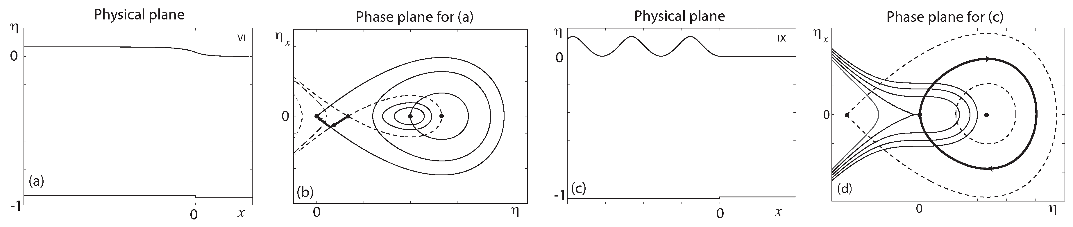
Solutions for flow types VI and IX are presented in Figure 7, and it is apparent that these two flow types were not possible with the two previous types of forcing (plate and bump) considered in this work. Examining solutions in the phase plane allows us to determine the flow type. For example, the solution shown in Figure 7b is for a waveless flow, with $F>1$ and $h>0$, which begins and ends its journey at the two saddle points in the phase plane. We need to determine the value of the upstream Froude number, $F_u$, that corresponds to the constant-level of the free-surface far upstream (i.e., the saddle point, ${\eta }_{-}=\eta (-\infty )$, given by Equation (27)), and this can be derived in a similar way to that of Equation (14) by using the transformation $\eta =\widehat{\eta }+{\eta }_{\pm }$ and Equation (26) to obtain

$$F_u=1\mp \sqrt{{(F-1)}^2-\frac{3}{2}h}\mathrm{for}{\eta }_{\pm },$$

(30)

which is a new approximation for the upstream Froude number, when $\sigma (-\infty )\ne \sigma (\infty )$. Note that Equations (27), (28) and (30) reduce to Equations (6), (7) and (14) when $\sigma (\pm \infty )=0$, or $h=0$. Continuing with our example, we have $F_u>1$ (with $\eta (-\infty )={\eta }_{-}$, $F>1$ and $h>0$) for the waveless flow type VI shown in Figure 7a. If we consider the limit as $h\to 0^{+}$, then ${\eta }_{-}\to 0^{+}$, and therefore this supercritical solution can be further classified as a perturbation of a uniform stream. It is worth mentioning that the analysis in the phase plane shows that the perturbation of a solitary wave sub-type solution does not exist in the case of a step in the channel bottom topography.

For flow over a step, Binder et al. [54] used the weakly nonlinear theory to determine the existence of the basic flow types III, IV, V, VI and IX. However, in this paper, we shall focus on solutions that are wave-free in the far-field and compare values from the weakly nonlinear analysis with exact values found in the full problem.

Exact solutions of the full problem for flow over a step that are wave-free in far-field must satisfy the relations [54]

$$F^2(1-{(1+\eta (-\infty )-h)}^2){=2(1-(1+\eta (-\infty ))(1+\eta (-\infty )-h)}^2,$$

(31)

and

$$F_u=F{(1+\eta (-\infty )-h)}^{-3/2},$$

(32)

with the maximum height of the step in the full problem being given by [51]

$$h=\frac{1}{2}(2+F^2-3F^{2/3}).$$

(33)

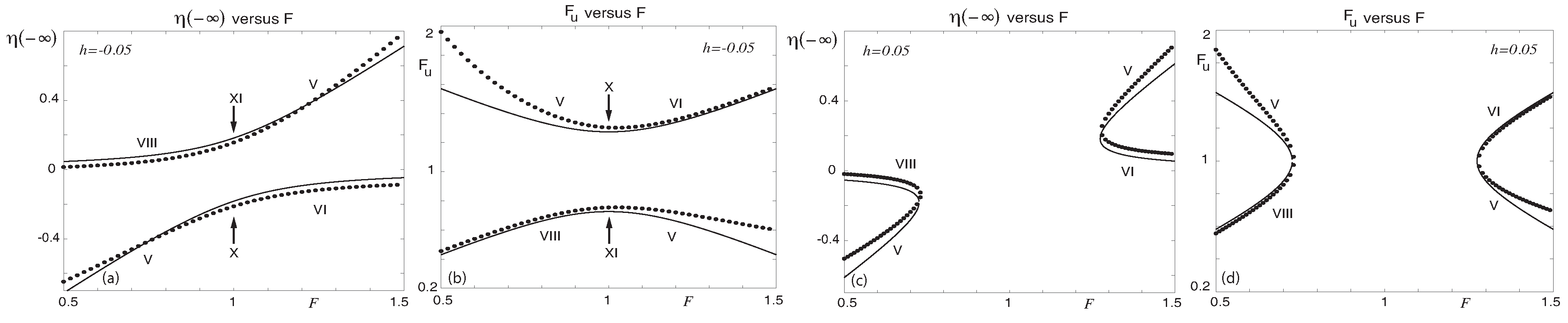
Note that Equations (31) and (32) relax to those of Equations (10) and (11) when $h=0$. The comparison between weakly nonlinear, Equations (27) and (30), and fully nonlinear, Equations (31) and (32), results for $h=\pm 0.05$ is presented in Figure 8, and qualitatively similar results are also found for other non-zero values of the step height, $h\ne 0$. In the case of when $h>0$, we see that there is a gap in the solution space around the value of $F=1$ in Figure 8c,d, and the turning points are given by Equations (29) and (33), which correspond to the maximum height of the step. The analysis presented in Figure 8 illustrates that only five out of the eight basic flow types that are wave-free in the far-field are possible when $h\ne 0$. If we recall the case of when $h=0$, in which four wave-free solutions are possible (see Figure 4), we see that the hydraulic fall flow type V is the only common wave-free solution that exists in both problems when either $h=0$, or $h\ne 0$. Similar to the discussion at the end of Section 3.1, for the results shown in Figure 4, it is important to recognise that the above analysis does not guarantee the existence of the five solutions that are wave-free in the far-field for flow over a step, it merely indicates the possibility of their existence in flows where $\sigma (-\infty )=h$ and $\sigma (\infty )=0$. For example, the flow types VIII, X and XI do not exist for flow over a (single) step [54]. This is because the analysis, presented in Figure 8, only depends on the horizontal level of the channel bottom far upstream and far downstream, and in general this is independent of the precise details of the disturbance in the channel, including the disturbance of a single step up, or step down in the channel bed topography at $x=0$ (e.g., see Figure 7). In other words, the analysis presented in Figure 4 and Figure 8 is applicable to more complicated flow configurations, where there may be a combination of the three types of disturbances (plate, bump and step) in the channel, with uniform flow as $x\to \pm \infty$. These types of flows, with multiple disturbances in the channel, are often referred to as hybrid flows.

3.5. Hybrid Flows

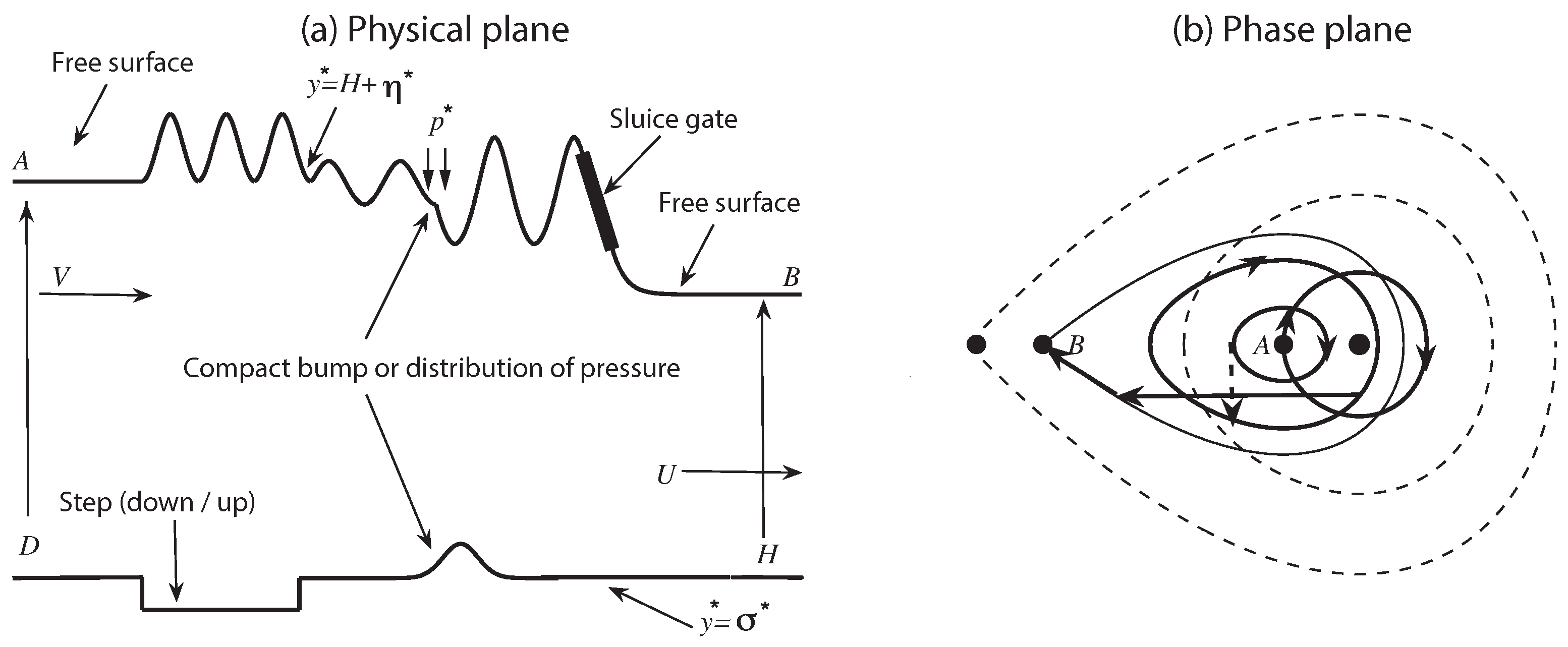
A hybrid flow refers to a problem when more than one of the disturbances (plate, bump and single step) are placed in the channel [28,33,35,44,50,56,57,58,59,84]. As the number of disturbances in the channel increases, identifying and classifying the types of flows becomes increasingly difficult, and is often counter-intuitive. The computation of a numerical solution to the hybrid flow problem requires the determination of the number of independent parameters in the numerical scheme and their approximate values. This has often been facilitated with prior knowledge and understanding on how to construct the solution in the weakly nonlinear phase space of the problem. In this work, we continue to focus on solutions that are wave-free in the far-field, with reference to the hybrid flows presented in Figure 2, Figure 9 and Figure 10.

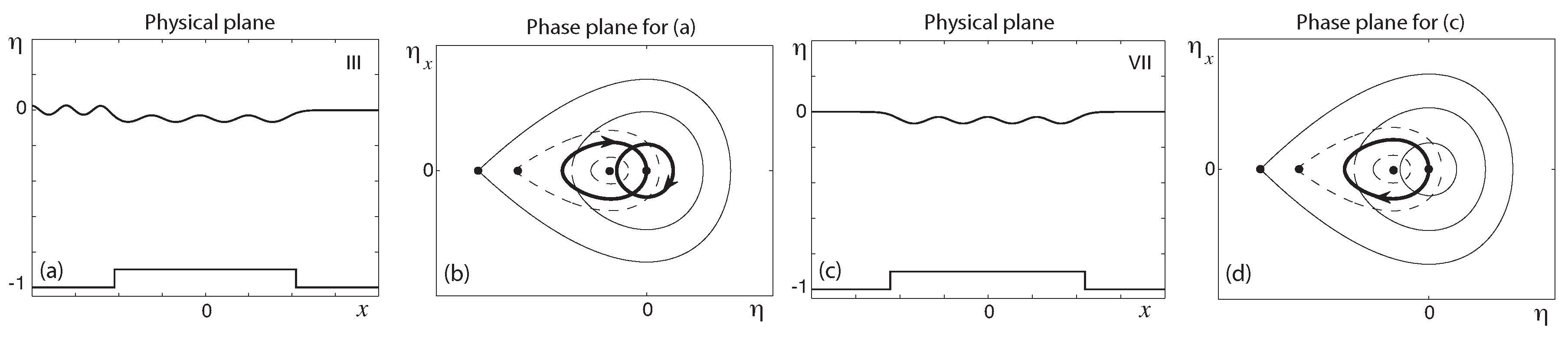
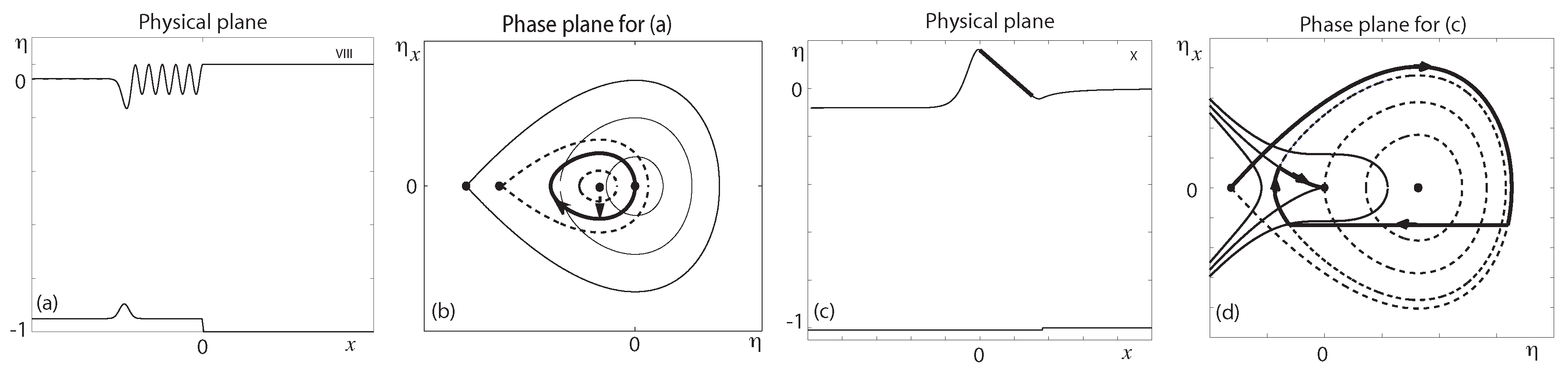
Figure 2 is an example of a hydraulic fall flow type V, which we have already discussed in the simpler problems of flow past a bump and (single) step (up or down) in the otherwise horizontal channel bed topography. Therefore, we shall begin our discussion in earnest with the results for subcritical flow over a long rectangular bump, or a step-up followed by a step-down (i.e., two steps), as is shown in Figure 9a,b. The periodic waves upstream of the long-bump correspond to the bold periodic orbit that encircles the centre located at the origin in the phase space. At the location of the upstream edge of the long-bump, there is a continuous movement to the bold period orbit that encircles the other centre, to the left of the origin in the phase space, and in physical space this corresponds to the waves located directly above the long-bump. At the location of the downstream edge of the long-bump, there is a continuous movement into the centre at the origin in phase space. The number of independent parameters for this solution is three, and it is an example of the basic flow type III. The parameters $F<1$ and $h>0$ determine both the general layout of the two phase planes (broken and solid curves, with four equilibria) and the amplitude of the waves directly above the bump, and the length of the bump, $B\gg 0$, determines the amplitude of the waves upstream of the long-bump. Note that the flow does not satisfy the radiation condition as there are waves entering system at $x=-\infty$, and this can be remedied by reversing the direction of the flow. Alternatively, we can eliminate the waves far upstream (see Figure 9c) by allowing the length of the bump to come as a part of the solution to ensure that the two continuous movements from the bold periodic orbit shown in Figure 9d are precisely away from and into the centre located at the origin in the phase space. Additionally, analysis in the phase space shows that the elimination of the waves far upstream does not occur for just one value of B, but rather a discrete set of values of B that are each approximately one wavelength apart. This is a non-trivial solution for subcritical flow type VII with uniform flow in the far-field, which can be further classified as a perturbation of a uniform subcritical stream (see Figure 3e and Figure 4b,c).

Hybrid solutions for the basic flow types VIII and X are presented in Figure 10. These two solution types are wave-free in the far-field and a comparison between weakly nonlinear approximations and exact solutions to the full problem is illustrated in Figure 8 (for values of $h=\pm 0.05$). We have now seen and discussed at least one example for each of the first ten basic flow types listed in the Introduction of this paper, and instead of presenting an example for the remaining eleventh basic flow type, we choose to discuss one way in which such a solution could be constructed.

Recall that the basic flow type XI is characterised by uniform flow in the far-field with $F>1$ and $F_u<1$. The analysis presented in Figure 4 and Figure 8 is therefore applicable to this flow type, and more specifically, Figure 8a,b show that $\sigma (-\infty )=h<0$. This means that we should examine the two phase planes corresponding to $F=1$ with $h<0$ and $h=0$ to see whether it is possible to construct a hybrid flow (e.g., see solid and broken curves in Figure 7d and Figure 10d). We also know that the solution must begin its journey at the (only) centre in the phase space for a value of $F_u<1$ (e.g., see Figure 7d). Therefore, the hybrid flow type XI could be obtained by simply introducing a small bump into the otherwise horizontal topography upstream of the step for the flow presented in Figure 7c,d. The precise location of the bump, $x_l<0$, and the amplitude of forcing, $A>0$, must then come as part of the solution to ensure that there is a vertical jump from the centre onto the periodic orbit that intersects with origin in the phase space (see Figure 7d). Although the location of the bump must come as part of the solution, it is not unique because the waves upstream of the bump can be eliminated for an infinite number of (unknown) discrete values of $x_l$, and hence it is possible to trap any number of waves in between the bump and step. It should now be clear that it is possible to construct hybrid flows for all eleven basic flow types I–XI.

4. Discussion

In this work, we have reviewed the phase plane analysis that can be used to establish the existence and non-existence of solutions for steady flow past four classical types of disturbances (plate, bump, compact distribution of pressure on the free surface and step) in an open channel. Solutions can be characterised using the eleven basic flow types I–XI, and analysis in the phase plane can help to further classify the sub-types of flows. For example, the basic supercritical flow type I for flow over a bump (with $A>0$) has two sub-type solutions–the perturbation of a solitary wave and perturbation of a uniform flow (see Figure 6).

For the eight basic solution types, I, II, V, VI, VII, VIII, X, XI, that are wave-free in the far-field, we compared approximations for weakly nonlinear values of the uniform flow conditions far upstream with exact values from the full problem to establish the possible existence of solutions for the disturbances considered in this work (see Figure 4 and Figure 8). The analysis, presented in Figure 4 and Figure 8, of solutions that are wave-free in the far-field depends on the horizontal level of the channel bottom as $x\to \pm \infty$, and this can be considered a global feature of a given flow configuration, which is independent of the precise details of any localised disturbances that are placed in the channel flow (e.g., hybrid solutions, with multiple disturbances in flow). The analysis of solutions that are wave-free in the far-field together with the phase plane analysis for the localised disturbances in the flow enabled us to classify all the possible solutions for a given disturbance(s), which is summarised in

Table 1. Summary of results.

Type of Disturbance(s)	Basic Flow Type
Plate	I and IV
Bump	I–V
Pressure	I–V
Step	III, IV, V, VI and IX
Hybrid (multiple disturbances)	I–XI

.

Numerical solutions of the full problem, which have been computed for all the weakly nonlinear solutions presented in this paper (see references in figure captions), and the analysis illustrated Figure 4 and Figure 8 provide quantitative measures to establish the range of validity of the weakly nonlinear analysis.

When within range of the weakly nonlinear analysis, the equilibria of the KdV equation give simple formulas Equation (27) for the uniform elevation of the free-surface far upstream. By transforming a constant non-zero level solution far upstream, i.e., the non-zero equilibria of the KdV equation, to the origin, we also derived a new, simple Equation (30) to approximate the upstream value of Froude number, $F_u$ (see Figure 4c and Figure 8b,d). We remark that for portions of the free surface that are wavy, or non-uniform, Equations (27) and (30) are useful approximations for the characteristic elevation of the free-surface and characteristic Froude number, $F_u$. For example, the fixed point that is the centre which is located to the left of the origin in the phase planes of Figure 9b,d, given by Equation (27) with $h>0$, is a measure of the mean free-surface elevation of the wavy portion of the flow directly above the long bump, and Equation (30) is then a measure of the average, or mean Froude number for this portion of the flow. Other quantities can also be easily approximated with the KdV analysis, such as the maximum elevation of the unforced solitary wave, length of plate, L, the maximum size of the bump, or amplitude of forcing, A, and maximum height of the step, h, (see Equations (9), (17), (23) and (29)).

In this paper, we have restricted our attention to four types of localised disturbances (flat plate, bump, pressure and step), and this localised property of the forcing in the non-autonomous system has enabled us to exploit a simpler, associated autonomous system—solutions were constructed in an autonomous phase plane with horizontal and vertical jumps between trajectories and fixed points, and the continuous movement from trajectories and fixed points of two autonomous phase planes. This methodology has potential application to other types of disturbances that we have not considered. For example, Binder et al. [30] considered flow with a curved plate and in the phase plane this gives a curved jump between trajectories and fixed points instead of the horizontal jump that we have seen for a flat plate. A similar approach has also been used to examine the waves in subcritical flow at the stern of a ship [11,85]. In these problems, the stern consists of a curved portion of the hull that is connected to a semi-infinite horizontal plate, which is assumed to have a constant pressure, P, applied to the plate as $x\to \infty$. Under these assumptions, the equations for a step Equations (26–28) with $h=P$ are the same as those for flow at the stern of a ship, and furthermore, Ogilat et al. [85] showed that an exact solution to Equation (28) is given in terms of Jacobian elliptic functions.

The success of the phase plane method relies on the localised nature of the forcing in the non-autonomous fKdV equation, even in hybrid flows with multiple (localised) disturbances. However, and more generally, the non-autonomous fKdV equation is not amenable to the phase plane method when the forcing is non-localised [84]. Nevertheless, in flows where the forcing is non-localised the fKdV is still a useful approximation to the full problem, and computing numerical solutions, or deriving further analytical approximations of Equation (4) can provide a way to explore the solution space in an efficient manner before attempting to compute solutions to the full problem [84]. Recently, the fKdV has been used to establish the existence of the five basic flow types I–V past finite and infinite length corrugations in the channel bed topography, which were confirmed with the computation of numerical solutions of the full problem [61,63,86]. With all these methods, the forcing, f, is prescribed in Equation (4) and we solve for the free-surface elevation, $\eta$. This is sometimes referred to as the forward problem. Alternatively, one can prescribe $\eta$ and solve for f, which is referred to as the inverse problem [10,19,35,45,60,61,80], and this is of interest in our ongoing research in this area.

The inverse problem has practical application to channel flows as the shape of the free-surface is usually observable or known, whereas the topography is unknown (e.g., in the case of a muddy stream). The fKdV Equation (4) is a very simple model for the inverse problem provided that $\eta$ is both differentiable and satisfies the conditions Equation (5). The unknown forcing, f, in the inverse problem is then simply an output of Equation (4) and therefore gives a straight-forward way to explore the inverse problem solution space, or at least a part of it. For example, Binder et al. [60,61] used the fKdV equation to examine the existence of solutions in the inverse problem. They also developed a rather general method, involving both inverse and forward approaches, to establish the non-uniqueness of solutions for the basic flow type II, which have been confirmed to exist in the full problem. Tam et al. [19] compared both weakly and nonlinear predictions for the inversely found forcing to the topography in experiments of two-dimensional hydraulic falls (flow type V, see Figure 1).

Since Russell’s observations of the Great Wave of Translation (i.e., the solitary wave) in 1834 that motivated the original model derivations of Boussinesq (1871), Rayleigh (1877) and Korteweg and de Vries (1895), the KdV equation has found application in many other areas of physical science, including collisionless-plasma magnetohydrodynamics, long waves in anharmonic crystals, the famous work of Zabusky [87] who discovered the soliton, and the rare meteorological phenomenon called the Morning Glory cloud [88]. There are also generalised, modified, extended and variable coefficient KdV equations, and the two-dimensional KdV equation, or Kadomtsev–Petviashvili (KP) equation [89]. The latter of these, the KP equation, is an approximation for the three-dimensional fully nonlinear problem, with slowing varying wave propagation in the spatial direction that is transverse to the main direction of the flow.

In closing, we recall that the basic hydraulic fall flow-type V has been shown to be a good approximation to the experimental flow over a bump in Figure 1 [19]. However, it is important to note that solutions of the time-dependent problem do not always evolve to a steady solution in the long-time limit. In the case of a bump, we have seen that the phase plane analysis predicts two regions of the solution space which are intrinsically unsteady, and time-dependent solutions, with an initially uniform and flat free-surface (i.e., $\eta (x,0)=0$ for $t=0$), do not evolve to a steady solution (see waterfall plots in Figure 6). Related to the time-dependent problem is the stability of steady solutions of the fKdV equation, and this has received considerable attention in many previous studies [25,32,34,49,52,55,61,70,71] (and others). If we again consider the case of a bump, the sub-type solutions Ib&c that are classified as a perturbation of a solitary wave are unstable, and the perturbation of a uniform stream solution Ia is stable (see [49] and others). The stability of the steady solutions is therefore important when interpreting the physical application of the results in this paper.