Abstract
We numerically solved the acoustic and flow field around cicada wing models with parametrically varied flexibility using the hydrodynamic/acoustic splitting method. We observed a gradual change of sound directivity with flexibility. We found that flexible wings generally produce lower sound due to reduced aerodynamic forces, which were further found to scale with the dynamic pressure force defined as the integration of dynamic pressure over the wing area. Unlike conventional scaling where the incoming flow velocity is used as the reference to calculate the force coefficients, here only the normal component of the relative velocity of the wing to the flow was used to calculate the dynamic pressure, putting kinematic factors into the dynamic pressure force and leaving the more fundamental physics to the force coefficients. A high correlation was found between the aerodynamic forces and the dynamic pressure. The scaling is also supported by previously reported data of revolving wing experiments.
1. Introduction
The flapping wing flight of insects has been under active research in the last decade. Part of the difficulty lies in the integration of many complex processes involved, including the kinematics of the deformable wings, the dynamics of the unsteady fluid flow, the structural mechanics of composite materials and the stable control of highly nonlinear systems. Another part lies in the diversity of the implementations of natural flyers. This work tries to contribute to this topic by investigating the correlation between the sound and force production in flapping wing flight of insects and the effect of wing flexibility.
For the aerodynamics of insect flight, Sun [1] published a comprehensive review recently. Conventional theory treats the aerodynamics of flapping motion in a quasi-steady way: the instantaneous aerodynamic forces on a flapping wing are equal to the forces during steady motion of the wing at an identical instantaneous velocity and angle of attack [2]. Its failure to calculate the average lift for hovering led to the finding of the unsteady mechanism of the leading-edge vortex [3] or the delayed stall mechanism. Other mechanisms were also found including the wing rotation, added mass effect and wake capture [4]. However, it was shown that the power requirement for the wing rotation mechanism is very high, indicating its limited application to maneuvers only [5]. Sun [1] further summarized that most of the aerodynamic force would be produced in the mid-portion of a half-stroke when the translation velocity is relatively high as a result of the delayed-stall mechanism. Revolving wing experiments [4,6,7] showed that the forces during the translation motion are generally normal to the wing surface and the force coefficients can be approximated as simple trigonometric functions of angle of attack. Dickinson et al. [8] experimented with the effect of advance ratio with revolving flat wing models, and showed that the trigonometric relationship between the force coefficient and angle of attack still holds for forward flight. The force production can be approximated with a revised quasi-steady model. Despite the application of these results in flight dynamics studies [1], the revolving wing models all have zero stroke plane angle, i.e., the stroke plane is horizontal, which is unrealistic, especially in forward flight.
It seems doubtless that the flapping of wings is for locomotion, and the sound it generates is incidental to the disturbance of air. However, insects were found to utilize the flight sound for purposes like sexual communication [9,10] and aposematic signals [11]. The acoustic communication of Drosophila was thought to be only possible over a short distance, which is not necessarily a disadvantage because it allows privacy of communication. Consequently, reduction in the flapping sound could be beneficial by avoiding predators and, more importantly, competitors [9]. For the swimming of fish, sometimes called “underwater flight”, sound produced by flapping fins is hypothesized to play a role in schooling, where a group of fish move in the same direction in a highly coordinated manner [12] and usually with complex yet swift change of patterns. This hypothesis is indirectly supported by later experimental findings that vision is not important in schooling of some fish species [13,14]. On the sensory side, both insects and fish have evolved specifically for sound detection. For example, the antennae of some fly species can respond to sounds physically similar to their own species [15] and the antennae of male mosquitoes are highly sensitive and can amplify female sounds [10]. The lateral line in fish is a system of sense organs responsible for detecting mechanical stimuli in the surrounding water, and when deprived, an individual’s ability to follow the school would be significantly undermined [14]. Therefore, the flapping sounds can be termed sonations [16] due to the evolved specialty. Research regarding this aspect would be helpful for understanding biological behaviors, as well as for developing ultra-quiet macro air vehicles. Previous experimental [17] and simulation works [18,19] on the sound production of flapping wings generally found that the flapping tone is directional and changes with flight conditions. Geng et al. [20] showed that the flapping tone is mainly generated by the fluctuating aerodynamic forces. The sound signal and the force signal were related in both radiation pattern and amplitude. It seems that the sound is inherently integrated with locomotion and some coordination by the insects is needed if they are to send signals while maintaining flight.
One common feature of insect and avian wings is that they are flexible and undergo time-varying deformations in motion. Since the flapping motion is actuated mainly at the wing base closer to the leading edge, the deformation is passively “controlled” through the structural properties and the flow–structure interaction process. Comparison between the deformation of flapping insect wings in air and helium [21] showed that the deformation is mainly due to wing inertia, which is reasonable given the massive acceleration during wing reversals. Building on this conclusion, the thinner trailing edge seems more for mass reduction than flexibility as the reduced inertia helps avoid excessive deformation which is detrimental for performance [22,23]. However, the comparison was only performed for one hawkmoth species (Manduca sexta), and thus the conclusion might not hold for species with wing structures deviating significantly. Therefore, this does not exclude the potential function of unique flexibility in natural wings. One prominent effect of flexibility is changing force direction with the changed face normal due to wing deformation [24]. Studies on the structural properties of corrugated insect wings have shown that because of the arrangement of the veins, in general, the flapping wing mainly has camber deformation and spanwise twist deformation [1], both of which were found beneficial for power economy [25,26]. Aside from the quantitative changes in aerodynamic forces and power requirements, flexibility is deemed to not affect the fundamental force production mechanism [1]. Geng et al. [20] showed that wing flexibility changes the directivity of the flapping tone and helps reduce the sound pressure level through reduced aerodynamic forces. However, the study is limited to only two cases, one using reconstructed cicada wing kinematics and the other using simple flapping kinematics. The reason for the reduction in aerodynamic forces was unclear.
The current study uses cicada wing models with prescribed kinematics reconstructed from high-speed photogrammetry to investigate the sound and force production of flapping wings. The three-dimensional (3D) incompressible flow field was solved with direct numerical simulation and the acoustic field was solved using linear perturbed compressible equations. The effect of flexibility was investigated using synthetic kinematics constructed with modes decomposed from the real kinematics. In this paper, we first discuss the sound production of the flapping wings with parametrically varying flexibility. We then discuss the force production from the perspective of dynamic pressure force scaling. The availability of the cicadas and their relatively large and transparent wings make them a good candidate for kinematics reconstruction. While the sound production of cicadas involving the tymbal has raised much more research interest, its flapping wing sound, to the best of our knowledge, remains unexplored. Here, it is used as a role model to help understand the sound and force production of flapping wings of insects in general.
2. Materials and Methods
2.1. Computational Methodology
To solve both the unsteady flow field and the acoustic field, the hydrodynamic/acoustic splitting method is adopted in the current study. In this splitting method, the instantaneous compressible flow variables are decomposed into the incompressible variables and the fluctuation about them as:
In Equation (1), are the incompressible density, flow velocity and pressure, while the primed/perturbed quantities are the fluctuations due to compressibility and can be regarded as acoustic variables in the far-field. The governing equations for the acoustic variables can be derived [27] by substituting the decomposition in Equation (1) into the governing equations of a compressible, viscous flow and subtracting the incompressible Navier–Stokes (INS) equations, which are given here in Equation (2).
Seo and Moon [28] proposed a revised formulation of the splitting method and derived a set of perturbed compressible equations (PCE) to better handle the near-field compressibility effect. A linearized version [29] of the PCE (LPCE) was further proposed to suppress the generation of perturbed vorticity, which makes the solution more grid-independent. The readers are referred to the work of Seo and Moon [28,29] for the derivation and verification. The set of LPCE is given here:
where γ is the ratio of the specific heats, and the DP/Dt term represents the sound source from the flow solver.
The LPCE is implemented in conjunction with our previous immersed-boundary method based flow solver [30,31] which is used to solve the INS. A sharp-interface method based on the ghost-cell approach is employed for boundary treatment to resolve the moving geometry of the cicada wing. The numerical implementation of the LPCE is the same as is described in reference [29]. The splitting method with the LPCE applies to low-Mach (Ma < 0.3) flows and has been verified and tested on canonical problems of flow-induced sound with Reynolds numbers ranging from 100 to 10,000. The readers are referred to the work by Seo and Mittal [32] for previous verification and application of this method, where it is demonstrated to be capable of solving the acoustic field in low-Mach flows involving complex geometry such as the human vocal tract and air-conditioning vents. We believe that the application of this method to the current case of flapping wing flight is appropriate because it falls under the category of low-Mach flows and the Reynolds number is comparable to the validated cases. Our previous study [20] also showed that the directivity of the computed sound from the flapping wings was comparable to experimental measurements [17].
2.2. Wing Models and Simulation Setup
The baseline cicada wing model used in this study is the same as that used in a previous study [20], to which the readers are referred for detailed description. For completeness, a brief description of the reconstruction method [33] and the wing kinematics are reproduced here. The wing and body positions of a cicada in free forward flight were recorded using a fully calibrated videography system from three orthogonal views. The images were taken at 1000 frames per second with a resolution of 1024 × 1024 pixels. Three-dimensional wing and body geometries were measured using all three orthogonal views of the cicada. The reconstruction method makes no rigid wing assumptions and allows for an arbitrary arrangement of marker points on the wing. The resulting wing surfaces are projected back into the image space to validate reconstruction accuracy. Figure 1 describes the key kinematic parameters with the wing positions at the beginning of the down- and up-stroke. The flight direction is towards the positive x axis. The angle between the mean stroke plane and the horizontal plane (the x–z plane) is 36°. The stroke amplitude is about 114° with the stroke angle (measured from the sagittal plane, or the x–y plane) starting from 22°. The mid-span chord length (c) of the cicada wing measures 19.6 mm with a wing span of 35 mm. The beating frequency (f) is about 46.5 Hz. The forward flight speed corresponding to this wing kinematic is 2.67 m/s. The Reynolds number is about 3500 based on the chord length and the forward flight speed, and about 16,500 based on the maximum wingtip velocity, which is about 12 m/s (Ma < 0.04).
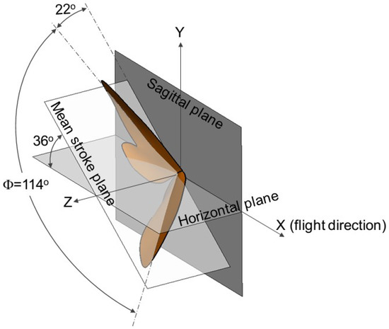
Figure 1.
Wing kinematics depicted with wing positions at the start of the each half-stroke. = stroke amplitude.
Besides the real wing motion that was reconstructed from a cicada in flight, other synthetic models (shown in Figure 2) were constructed using the first two principle modes (M1 and M2) that were extracted from the wing kinematics using the method of single value decomposition [34]. M1 is the most dominant mode, consisting of a simple flapping motion in the stroke plane, which contains about 80% of the total kinetic energy. M2 is a mode of wing morphing that contains about 15% of the kinetic energy. The construction follows the formula , where a is a constant coefficient. When a = 0, the model becomes roughly a rigid model. Thus, M1 and the rigid wing model are used interchangeably in this paper. Figure 2 shows the trajectories of the real motion as well as the synthetic wing models during the down-stroke and up-stroke with evenly spaced snapshots in time. Compared to the real wing motion, the rigid wing model has the same mean stroke plane and stroke angle. The difference is that the morphing mode is absent. The wing does not twist about the span axis and remains almost perpendicular to the mean stroke plane during the entire stroke cycle. Other models where a > 0 have different degrees of the morphing mode, which represents the degree of flexibility. The synthetic wing kinematics serve as models for comparative study rather than represent realistic flight conditions.
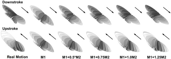
Figure 2.
Wing trajectory for the real and synthetic kinematics during downstroke (top row) and upstroke (bottom row) with evenly spaced snapshots in time. M1 = principle mode 1. M2 = principle mode 2.
The computational domain for the wing model is shown in Figure 3a. It is a cube with a side length of 200c. Since resolving the flow requires a much finer grid than resolving the acoustic field, grid-independent studies were performed by comparing the wing drag and lift histories with previous aerodynamic studies using similar wing models [35]. The final grid used in this study is a non-uniform Cartesian grid with 257 × 257 × 257 grid points. Figure 3b compares the computed lift coefficient between the current grid and a finer grid used in the previous study. It is calculated using , where is the lift force, ρ is the air density and is the mean wing tip velocity. The current grid is deemed good enough with the difference in the peak and valley values of the lift coefficient being less than 5% and the difference in their position also being less than 5%. The grid was not further increased to keep the computational cost affordable. The cicada wing is placed at the center of the domain, where a cubic region of about 8c side length is discretized with high-resolution uniform grids of 0.075c intervals to resolve the near-field flow. Outside the center uniform region, the grid is stretched to extend to the outer boundary with the same grid spacing used in all six directions. Previous studies [35,36] have shown that a domain size of about 30c is large enough to achieve an accurate flow solution. The large domain used here is able to resolve the flapping sound in the far field. The same setup was used in a previous work [20].
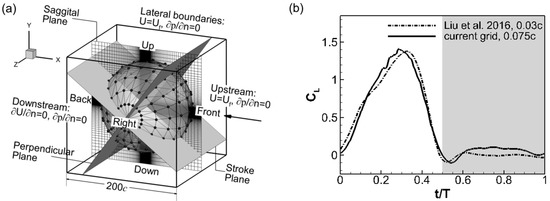
Figure 3.
(a) The computational doamin, boundary conditions, acoustic probe (black dots) setup and the reference planes and positions. (b) Comparison of the lift coefficient computed with two different grids.
For the flow solver, a uniform constant velocity was specified at the upstream boundary and the four lateral boundaries (Different were simulated to get the wing forces under different forward flight speeds). At the downstream boundary, a zero-gradient velocity condition was specified. For the pressure, a homogeneous Neumann condition was used at all the boundaries. For the acoustic solver, energy transfer and annihilating boundary conditions are used to model the outgoing acoustic waves at all the boundaries. On the solid surface (wing surface), a slip, adiabatic wall boundary condition [29] is used. The simulation was carried out with 480 flow time steps per cycle. Within each flow time step, the acoustic field was solved for 30 time steps.
To monitor the acoustic waves, acoustic probes were setup in the domain to continuously record the sound signal just like the microphones used in the experiments. The probes were arranged on a set of spherical surfaces centered at the fixation point of the wing root. Each monitor surface had 20 intervals in the latitudinal direction and 10 in the longitudinal direction with a total of 182 probe points. For example, Figure 3a shows the monitor spherical surface with a radius of 75c. The acoustic signal was sampled 960 times per cycle, i.e., at a frequency of 44,640 Hz.
Also shown in Figure 3a are the planes that are used to describe the spatial pattern of the flapping sound in the discussion. The reference planes (i.e., the sagittal plane, the mean stroke plane, and the plane that is perpendicular to both) are chosen based on their correlation with the wing kinematics.
3. Results and Discussion
In this section, we first discuss the characteristics of the flapping sound and its systematical change with wing flexibility. In the second part, we discuss the production of aerodynamic forces with wing kinematics of different flexibilities under various flight speeds. The scaling between the aerodynamic force and the dynamic pressure force is revealed.
3.1. Generation of the Flapping Tune
Data analysis of the acoustic signals is similar to that in reference [20]. Here it is applied to all the cases with parametrically varied wing flexibility. The simulation was run for a total of nine cycles for the real-motion and rigid wing models. The acoustic pressure signals recorded at the probes for the last six cycles were processed using fast Fourier transform (FFT) to obtain the frequency composition. The amplitude of each frequency component (harmonic) was then converted into sound pressure level (SPL) with respect to the reference pressure pref = 2.0 × 10⁻⁵ Pa. It was found during the process that using the acoustic data of the first four cycles as the FFT input would result in the same radiation pattern. Thus, for the rest of the wing models, each simulation was run for four cycles to save the computational expense. Clear radiation patterns were observed at about r = 10c and remained the same further from the wing [20]. For the rest of the paper, the analysis will focus on the spherical surface of r = 75c.
With the 3D simulation, polar plots of the sound amplitude variation around the wing can be readily extracted in any planes of interest. Figure 4 compares the juxtaposition of each harmonic of different models in the three reference planes. The corresponding monitor profile is shown at the left side to help visualize the relative position between the wing and the reference plane. Note that the monitor profile does not reflect the real distance between the wing and the monitors, which is 75c.
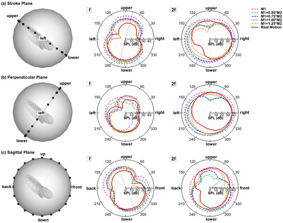
Figure 4.
Juxtapostion of sound pressure level (SPL) (dB) distribution of all the models for each of the the harmonics at r = 75c in the (a) stroke plane; (b) perpendicular plane; (c) saggital plane.
In the stroke plane, a general pattern can be observed: f is dipole-like and 2f is more monopole-like with a lower value at the upper side. It is also found that 2f dominates the sound spectrum at the right and left sides while f dominates the upper and lower sides. The same radiation pattern was reported in the experiment by Sueur et al. [17]. In the experiment, they described both the directional radiation pattern and the detailed frequency composition of the sound produced by a tethered fly (Lucilia sericata). The sound was recorded in the horizontal plane around the fly. Their analysis of the recorded sound showed that the first harmonic (f) formed a dipole-like pattern and dominated (having larger amplitude) in the front, whereas the second harmonic (2f) formed a monopole-like pattern and dominated at the sides. All models share the same angle between the dipole axis of f and the sagittal plane. The dipole axis is roughly perpendicular to the bisector of stroke amplitude . This shows that this angle is related to the stroke angle, which is the same for all the models. However, such an angle should not exist if two wings are simulated together due to the left–right symmetry.
In the perpendicular plane, 2f generally shows a monopole shape for all the models with the left and right sides being slightly stronger than the top and bottom sides. The shapes for f are quite irregular. Nevertheless, it is very clear that almost all the f plots are enveloped inside the 2f plots—an evidence of the 2f dominance at the sides.
In the sagittal plane (up–down–front–back), the change of the dipole axis of f can be observed. Whereas the rigid wing has the dipole axis aligned with the stroke plane, the flexible wings have it rotated towards the vertical axis, and the angle of rotation varies with the flexibility of the wing. Besides, the lower half of the 8-like shape is generally stronger than the upper half in the flexible wing models, especially in the real case. This “downstroke dominance” of the 8-like shape was also observed in the experiments of Sueur et al. [17]. Generally, the changes in 2f with flexibility are less clearly reflected in the 2D polar plots, mainly because the directions are no longer aligned well with the three reference planes.
Besides the changes in the radiation directivity, the flexible wings are generally observed to have lower SPL in all directions for both f and 2f. As shown in Figure 4, in the three reference planes, the envelopes of all the flexible models are basically contained in the envelope of the rigid model. This implies that the flexibility of the wing is beneficial for reducing flight noise. Corresponding to this, the flexible models generally have smaller aerodynamic forces as is shown in Figure 5. One interesting point is that the real motion model still has a lower sound than the M1 + 1.0M2 model, and different directivities. This indicates that higher modes might be important on noise reduction even though they are shown to be less important aerodynamically [34].

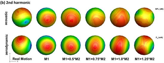
Figure 5.
Comparison of acoustic signal pattern (top row) and aerodynamic signal (bottom row) pattern for the stroke frequency (a) and the second harmonic (b) (note different contour levels are used for different models to compare the pattern for the second harmonic).
Geng et al. showed high correlation between the acoustic signal and the aerodynamic forces of the wings [20]. Here we use the same method to illustrate the correlation for the parametric cases. FFT analysis was performed on the forces to get the frequency composition of the aerodynamic forces. The force vector was first projected onto the normal direction at each probe point on the spherical surface using
where the aerodynamic signal is the normal component of the force coefficient vector at each probe point identified by the vector that points from the center of the sphere to the probe point. The aerodynamic signal at each probe point was then used as the input for the FFT.
Figure 5 compares the acoustic signal pattern and aerodynamic signal pattern of the wing models. It can be observed that the acoustic signal pattern highly matches the aerodynamic signal pattern for both f and 2f for all the wing flexibility. For f, the direction of the dipole axis of the acoustic singal are aligned with that of the aerodynamic signal. Besides the same directivity, signal strength is also related between the sound and the aerodynamic force: the rigid model has the strongest sound singal and aerodynamic force, while other models with increased flexibility have lower strength forces. This suggests that the main mechanism of noise reduction with flexibility is via reduced aerodynamic force. The same can be said for 2f, only that the alignment of acoustic and aerodynamic patterns are to a lesser degree. One reason behind this is that the aerodynamic force coefficient combines the pressure on both sides of the wing surface into a single parameter, and with the projection, the aerodynamic pattern is inherently symmetric, which is not true for the acoustic signal. Nevertheless, the peak and valley positions in the acoustic pattern are well predicted by the aerodynamic pattern. For the real-motion model and the M1 + 1.0M2 model, the aerodynamic forces are very close (as will be revealed in the next section), yet the radiation pattern of 2f of the two are very different. This indicates that small changes in the aerodyanmic force might have a large effect on the directivity of the flapping sound, which provides the possibility of sound modulation by insects while maintaining flight.
3.2. Aerodynamic Force Scaling with Dynamic Pressure Force
What has caused the reduced aerodynamic forces in the flexible models? Revolving wing experiments [4,6,7] showed that the forces during translation motion are generally normal to the wing surface. With flexible wings, the surface normal is changing within the flapping cycle due to the deformation and consequently the direction of the resultant force [37]. To quantify the effect of changing surface normal on the aerodynamic force of the flexible wings, we calculated the dynamic pressure force for all the cases, which is defined as
where is the local relative velocity between a point on the wing and the incoming flow. Note that is computed as a vector. The physical idea behind this formula is simple: the normal component of the relative velocity stalls to form the dynamic pressure force. The calculation also considers the direction of the dynamic pressure force which might not be uniform over the wing, especially during up-strokes, similar to the retreating blade of helicopters at high advance ratios where the base of the blade experiences backwards flow [38]. We plotted the aerodynamic force and the dynamic pressure force for all the wing models tested in this study in Figure 6 (note that the scale of the y-axis is different for each plot). The aerodynamic forces generated by the wing models were found to scale with the dynamic pressure force: the aerodynamic forces follow the trend of the dynamic pressure force in all three directions and reach peak values and change signs around the same time. We further tested other speeds for the rigid and real motion models. The same scaling is also observed at these two speeds (Figure 7).
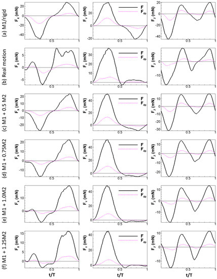
Figure 6.
Aerodynamic forces of the wing compared to dynamic pressure force for all the tested models under = 2.67 m/s.
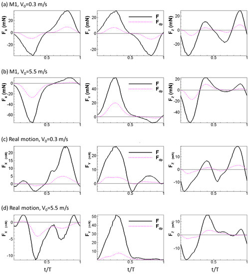
Figure 7.
Aerodynamic forces of the wing compared to dynamic pressure force for the rigid model and the real model under = 0.3 m/s and 5.5 m/s.
Figure 8 compares the aerodynamic forces and the dynamic pressure forces in the three directions among the models of different flexibility. The general trend is that more flexible wings have smaller forces. Comparing Figure 8a,b, we can see that the relative magnitudes among the models are generally similar for the aerodynamic forces and the dynamic pressure force. For example, in the x direction, the order for the magnitude of the aerodynamic force is M1 > M1 + 0.5M2 > M1 + 0.75M2 > M1 + 1.0M2 > M1 + 1.25M2. The same can be said for forces in the other two directions for both down-stroke and up-stroke, with the exception of the y direction for the down-stroke where the flexible models showed smaller dynamic pressure forces but higher aerodynamic forces than the rigid motion model. This indicates that although the kinematics in the flexible wing models reduce the dynamic pressure force, they maintain the high lift during down-stroke. The reason for this is likely to be that the primary lift generation mechanism during down-stroke is the leading-edge vortex, which is affected by the vortex dynamic rather than the dynamic pressures.
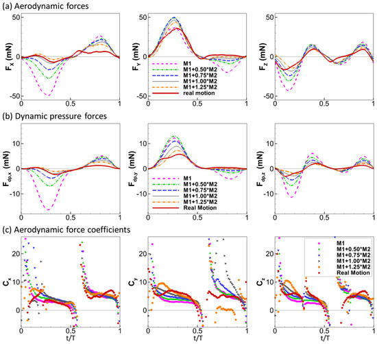
Figure 8.
Aerodynamic forces (a), dynamic pressure forces (b) and aerodynamic force coefficients (c) in the three directions.
Using the dynamic pressure force as a reference, the force coefficients are calculated as
where i is one of the three directions. The force coefficients thus calculated are plotted in Figure 8c for all the models. Generally, the force coefficients are close among the models. Significant differences occur near singularity points where the aerodynamic forces change signs. The largest difference among the models is found for Cy during the up-stroke, which might be partly due to the large relative error when the amplitude of the forces is close to zero. Among the models, the aerodynamic force coefficients of the rigid model are closest to constants throughout the mid-portion of each stroke.
The strong similarity between the curves of aerodynamic forces and the dynamic pressure forces is not reflected well by the force coefficients Ci. Therefore, we calculated the Pearson’s linear correlation coefficients between the aerodynamic forces and the dynamic pressure forces. The values are listed in Table 1 and Table 2 for all the cases tested in the current study. We can see that for all the tested cases, the R values are very close to one, indicating strong linear correlation between the aerodynamic forces and the dynamic pressure forces.

Table 1.
Linear correlation coefficients between the aerodynamic forces and the dynamic pressure forces at baseline forward speed (2.67 m/s).
Table 2.
Linear correlation coefficients between the aerodynamic forces and the dynamic pressure forces for the rigid and real model at different forward speeds.
Back to the question asked at the beginning of this section, what has caused the reduced aerodynamic forces in the flexible wings? We hypothesize that the flexible wing reduces the aerodynamic force mainly by reducing the dynamic pressure force through the changes of the surface normal. The change of the surface normal has two effects on the dynamic pressure force. The first is that the direction of the resultant force is changed [37]. This is represented by the in Equation (5). The second is that the normal component of the relative velocity is also changed, which is represented by the in Equation (5).
With the scaling being observed in different wing models at various speeds, we expect it to be a general principle that can be applied to the flapping motion of thin flat plates. We now discuss how well the scaling matches the data reported for revolving wing models. For a thin flat wing revolving in the horizontal plane, the force coefficients are usually calculated with the reference , where is the relative velocity and is the surface area of the wing. For example, for the vertical force, or lift, the equation can be written as
For a wing revolving in stationary air, the relative velocity changes from wing base to wingtip. A more accurate reference can be used by taking this into account and calculating the force coefficient with
This force coefficient is normally a function of the angle of attack. For the same wing, if we use the dynamic pressure force (for the vertical force, the vertical component is used) as a reference:
Comparing the two, we can see that . If is close to a constant, as is observed in Figure 8c in the rigid model case, then should scale with , i.e.,
Previous experiments of revolving wings also showed that the force coefficients could be fitted by trigonometric functions of angle of attack. But the specific forms vary. Dickson et al. [4] proposed the scaling relation
Another similar scaling relation was also proposed [8] based on data of revolving wings under various advance ratios as
In Figure 9, we compare the above three scaling relations against the experimental data by Usherwood and Ellington [7]. Equation (11) is a mathematical fit without physical meaning to it. In Equation (12), the term can be regarded as the vertical component of the normal force, but there seems to be no direct physical meaning for why the normal force scales with . One possible explanation is that the whole velocity stalls to form the dynamic pressure on the surface, and indicates the component of the dynamic pressure force normal to the surface. In their experiment, Dickinson et al. [8] took the chord-wise component of the incoming flow velocity, suggesting that only the normal component stalls. For Equation (10), however, the term arises from the normal component of the velocity. Equation (12) is symmetric about α = 45° and Equation (11) is very close to Equation (12) in terms of the shape. Due to the square of , Equation (10), however, gets the peak value at about α = 55°. The curves obtained by Usherwood and Ellington [6,7] in various models generally show asymmetry about α = 45°and reach the peak value at a slightly higher angle of attack. Equation (10) best captures the asymmetry, and the scaling factor used to match the amplitude of experimental data (3.63) is very close to the one observed in the cicada case shown in Figure 8c. This indicates that the dynamic pressure force scaling generally applies to the force production of thin plate flapping/revolving motion. One problem is its prediction of force coefficients at lower angles of attack is smaller than the experimental data. The condition for this scaling to work is that the resultant force needs to be normal to the surface, which is not true when the angle of attack is low due to the viscous effect [4,8]. The viscous effect is more dominant when Re is smaller, which probably explains why Dickson et al. obtained a symmetric scaling while the data of Usherwood and Ellington [6,7] shows asymmetry, since a higher Reynolds number was used in the latter (Re 1100–26,000) compared to Re ≈ 140 by Dickinson et al. [4,8].
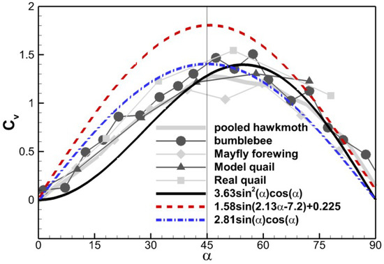
Figure 9.
Comparison of scaling relations with experimental data digitalized from Figure 8b, Usherwood and Ellington [7].
4. Conclusions
The current study uses cicada wing models with prescribed kinematics reconstructed from high-speed photogrammetry to investigate the sound and force production of flapping wings. The three-dimensional (3D) incompressible flow field is solved with direct numerical simulation and the acoustic field is solved using linear perturbed compressible equations. The flexible models were found to generate lower sound due to lower aerodynamic forces produced by the wings. The directivity of the flapping tone is found to change gradually with wing flexibility. The aerodynamic forces were found to scale with the dynamic pressure force, which is defined as the integral over the wing area of the dynamic pressure calculated from the normal component of the relative velocity. Since the dynamic pressure force is determined solely by the kinematics, it can be directly computed for different flapping flight configurations without computational fluid dynamics (CFD) simulation to predict the force generation. Such scaling would be useful for understanding a variety of flapping kinematics under different flight conditions. It could also be useful in the drafting stage of flapping wing micro air vehicle design, since the aerodynamic forces can be roughly estimated using only the wing kinematics and the flight condition without any CFD simulation needed. The current findings can be helpful in understanding insect behaviors involving flight and sound production. For example, based on the correlation between the force and sound production, it can be inferred whether the change in kinematics under certain scenarios is used to alter the radiated sound.
Author Contributions
Conceptualization, X.Z.; methodology, X.Z. and Q.X.; software, X.Z. and Q.X.; formal analysis, X.Z., Q.X. and B.G.; investigation, B.G.; resources, G.L. and H.D.; data curation, B.G.; writing—original draft preparation, B.G.; writing—review and editing, Q.X., G.L. and H.D.; visualization, B.G.; supervision, Q.X.
Funding
This research received no external funding.
Acknowledgments
The authors would like to thank the Advanced Computing Group at the University of Maine for providing the computational resource and technical support.
Conflicts of Interest
The authors declare no conflict of interest.
References
- Sun, M. Insect flight dynamics: Stability and control. Rev. Mod. Phys. 2014, 86, 615. [Google Scholar] [CrossRef]
- Ellington, C.P. The aerodynamics of hovering insect flight. I. The quasi-steady analysis. Philos. Trans. R. Soc. Lond. B Biol. Sci. 1984, 305, 1–15. [Google Scholar] [CrossRef]
- Ellington, C.P.; Van Den Berg, C.; Willmott, A.P.; Thomas, A.L.R. Leading-edge vortices in insect flight. Nature 1996, 384, 626. [Google Scholar] [CrossRef]
- Dickinson, M.H.; Lehmann, F.-O.; Sane, S.P. Wing Rotation and the Aerodynamics Basis of Insect Flight. Science 1999, 284, 1954–1960. [Google Scholar] [CrossRef] [PubMed]
- Sun, M.; Tang, J. Lift and power requirements of hovering flight in Drosophila virilis. J. Exp. Biol. 2002, 205, 2413–2427. [Google Scholar] [PubMed]
- Usherwood, J.R.; Ellington, C.P. The aerodynamics of revolving wings I. Model hawkmoth wings. J. Exp. Biol. 2002, 205, 1547–1564. [Google Scholar] [PubMed]
- Usherwood, J.R.; Ellington, C.P. The aerodynamics of revolving wings II. Propeller force coefficients from mayfly to quail. J. Exp. Biol. 2002, 205, 1565–1576. [Google Scholar] [PubMed]
- Dickson, W.B.; Dickinson, M.H. The effect of advance ratio on the aerodynamics of revolving wings. J. Exp. Biol. 2004, 207, 4269–4281. [Google Scholar] [CrossRef] [PubMed]
- Ewing, A.W. Arthropod Bioacoustics: Neurobiology and Behaviour; Comstock Publishing Associates: Ithaca, NY, USA, 1989. [Google Scholar]
- Jackson, J.C.; Robert, D. Nonlinear auditory mechanism enhances female sounds for male mosquitoes. Proc. Natl. Acad. Sci. USA 2006, 103, 16734–16739. [Google Scholar] [CrossRef] [PubMed]
- Srygley, R.B. Evolution of the wave: Aerodynamic and aposematic functions of butterfly wing motion. Proc. R. Soc. Lond. B Biol. Sci. 2007, 274, 913–917. [Google Scholar] [CrossRef] [PubMed]
- Pitcher, T.J. Behaviour of Teleost Fishes; Fish & Fisheries Series; Springer: Dordrecht, The Netherlands, 1992; ISBN 9780412429309. [Google Scholar]
- Pitcher, T.J.; Partridge, B.L.; Wardle, C.S. A blind fish can school. Science 1976, 194, 963–965. [Google Scholar] [CrossRef] [PubMed]
- Partridge, B.L.; Pitcher, T.J. The sensory basis of fish schools: Relative roles of lateral line and vision. J. Comp. Physiol. 1980, 135, 315–325. [Google Scholar] [CrossRef]
- Robert, D.; Göpfert, M.C. Acoustic sensitivity of fly antennae. J. Insect Physiol. 2002, 48, 189–196. [Google Scholar] [CrossRef]
- Clark, C.J. Locomotion-Induced Sounds and Sonations: Mechanisms, Communication Function, and Relationship with Behavior. In Vertebrate Sound Production and Acoustic Communication; Suthers, R., Fitch, W., Fay, R., Popper, A., Eds.; Springer Handbook of Auditory Research; Springer: Cham, Switzerland, 2016; Volume 53. [Google Scholar]
- Sueur, J.; Tuck, E.J.; Robert, D. Sound radiation around a flying fly. J. Acoust. Soc. Am. 2005, 118, 530–538. [Google Scholar] [CrossRef] [PubMed]
- Bae, Y.; Moon, Y.J. Aerodynamic sound generation of flapping wing. J. Acoust. Soc. Am. 2008, 124, 72–81. [Google Scholar] [CrossRef] [PubMed]
- Inada, Y.; Aono, H.; Liu, H.; Aoyama, T. Numerical Analysis of Sound Generation of Insect Flapping Wings. Theor. Appl. Mech. Jpn. 2009, 57, 437–447. [Google Scholar]
- Geng, B.; Xue, Q.; Zheng, X.; Liu, G.; Ren, Y.; Dong, H. The effect of wing flexibility on sound generation of flapping wings. Bioinspir. Biomim. 2017, 13, 16010. [Google Scholar] [CrossRef] [PubMed]
- Combes, S.A.; Daniel, T.L. Into thin air: Contributions of aerodynamic and inertial-elastic forces to wing bending in the hawkmoth Manduca sexta. J. Exp. Biol. 2003, 206, 2999–3006. [Google Scholar] [CrossRef] [PubMed]
- Eldredge, J.D.; Toomey, J.; Medina, A. On the roles of chord-wise flexibility in a flapping wing with hovering kinematics. J. Fluid Mech. 2010, 659, 94–115. [Google Scholar] [CrossRef]
- Heathcote, S.; Wang, Z.; Gursul, I. Effect of spanwise flexibility on flapping wing propulsion. J. Fluids Struct. 2008, 24, 183–199. [Google Scholar] [CrossRef]
- Kang, C.-K.; Aono, H.; Cesnik, C.E.S.; Shyy, W. Effects of flexibility on the aerodynamic performance of flapping wings. J. Fluid Mech. 2011, 689, 32–74. [Google Scholar] [CrossRef]
- Du, G.; Sun, M. Effects of wing deformation on aerodynamic forces in hovering hoverflies. J. Exp. Biol. 2010, 213, 2273–2283. [Google Scholar] [CrossRef] [PubMed]
- Young, J.; Walker, S.M.; Bomphrey, R.J.; Taylor, G.K.; Thomas, A.L.R. Details of insect wing design and deformation enhance aerodynamic function and flight efficiency. Science 2009, 325, 1549–1552. [Google Scholar] [CrossRef] [PubMed]
- Hardin, J.C.; Pope, D.S. An acoustic/viscous splitting technique for computational aeroacoustics. Theor. Comput. Fluid Dyn. 1994, 6, 323–340. [Google Scholar] [CrossRef]
- Seo, J.-H.; Moon, Y.J. Perturbed compressible equations for aeroacoustic noise prediction at low Mach numbers. AIAA J. 2005, 43, 1716–1724. [Google Scholar] [CrossRef]
- Seo, J.H.; Moon, Y.J. Linearized perturbed compressible equations for low Mach number aeroacoustics. J. Comput. Phys. 2006, 218, 702–719. [Google Scholar] [CrossRef]
- Mittal, R.; Dong, H.; Bozkurttas, M.; Najjar, F.M.; Vargas, A.; von Loebbecke, A. A versatile sharp interface immersed boundary method for incompressible flows with complex boundaries. J. Comput. Phys. 2008, 227, 4825–4852. [Google Scholar] [CrossRef] [PubMed]
- Zheng, X.; Xue, Q.; Mittal, R.; Beilamowicz, S. A coupled sharp-interface immersed boundary-finite-element method for flow-structure interaction with application to human phonation. J. Biomech. Eng. 2010, 132, 111003. [Google Scholar] [CrossRef] [PubMed]
- Seo, J.H.; Mittal, R. A high-order immersed boundary method for acoustic wave scattering and low-Mach number flow-induced sound in complex geometries. J. Comput. Phys. 2011, 230, 1000–1019. [Google Scholar] [CrossRef] [PubMed]
- Koehler, C.; Liang, Z.; Gaston, Z.; Wan, H.; Dong, H. 3D reconstruction and analysis of wing deformation in free-flying dragonflies. J. Exp. Biol. 2012. [Google Scholar] [CrossRef] [PubMed]
- Ren, Y.; Dong, H. Low-dimensional Modeling and Aerodynamics of Flexible Wings in Flapping Flight. In Proceedings of the 34th AIAA Applied Aerodynamics Conference, Washington, DC, USA, 13–17 June 2016; p. 4168. [Google Scholar]
- Liu, G.; Dong, H.; Li, C. Vortex dynamics and new lift enhancement mechanism of wing–body interaction in insect forward flight. J. Fluid Mech. 2016, 795, 634–651. [Google Scholar] [CrossRef]
- Wan, H.; Dong, H.; Gai, K. Computational investigation of cicada aerodynamics in forward flight. J. R. Soc. Interface 2014, 12, 20141116. [Google Scholar] [CrossRef]
- Zhao, L.; Huang, Q.; Deng, X.; Sane, S.P. Aerodynamic effects of flexibility in flapping wings. J. R. Soc. Interface 2010, 7, 485–497. [Google Scholar] [CrossRef] [PubMed]
- Leishman, G.J. Principles of Helicopter Aerodynamics with CD Extra; Cambridge University Press: New York, NY, USA, 2006. [Google Scholar]


© 2018 by the authors. Licensee MDPI, Basel, Switzerland. This article is an open access article distributed under the terms and conditions of the Creative Commons Attribution (CC BY) license (http://creativecommons.org/licenses/by/4.0/).