A Review of Methodology for Evaluating the Performance of Atmospheric Transport and Dispersion Models and Suggested Protocol for Providing More Informative Results

Abstract

Many models exist for predicting the atmospheric transport and dispersion of material following its release into the atmosphere. The purpose of these models may be to support air quality assessments and/or to predict the hazard resulting from releases of harmful materials to inform emergency response actions. In either case it is essential that the user understands the level of predictive accuracy that might be expected. However, contrary to expectation, this is not easily determined from published comparisons of model predictions against data from dispersion experiments. The paper presents and reviews the methods adopted and issues involved in comparing the predictive performance of atmospheric transport and dispersion models to experimental data, by reference to a number of experimental data sets and comparison results. It then presents an approach which is designed to make the performance of atmospheric dispersion models more transparent, through clearly defining the basis on which the comparison is made, and comparing the performance of the chosen model to that of a reference model. Such an approach establishes a clear baseline against which the accuracy of models can be evaluated and the performance benefits of more sophisticated approaches quantified. The use of a simple analytic reference model applicable to continuous ground level releases in open terrain and urban areas is shown as a proof-of-principle.

1. Introduction

The need to be able to predict urban air quality, regulate emissions from industrial plants and predict the consequences of unexpected releases of hazardous materials, has led to the development of a large number of atmospheric transport and dispersion (AT&D) models of varying levels of complexity. However, in order for these models to be applied with confidence it is necessary to demonstrate their fitness-for-purpose, through some form of evaluation process. This had led to the development of a wide range of metrics and a significant body of literature on the results of model comparisons. It has also led to the development of initiatives, such as harmonisation within atmospheric dispersion modelling for regulatory purposes (HARMO), in order to promote the standardisation and development of AT&D models, and the development of best practice guides and model evaluation protocols, such as that developed under the Cooperation in Science and Technology Action 732 [1].

The purpose of the present paper is to highlight the challenges involved in fully understanding the performance of a particular dispersion model by reviewing:

• The wide range of AT&D models available the differences between them and how these and limitations in our physical understanding may affect model evaluations;
• The range of performance metrics typically used in model evaluations;
• The limitations inherent in comparisons made against data obtained from field and wind tunnel experiments;
• How decisions in the evaluation process affect the results.

It is then suggested that to make evaluations more informative, comparison with a universally recognised reference model should be an essential part of any evaluation protocol.

2. Types of AT&D Model

AT&D models range from simple analytic Gaussian plume models, to numerical models based on sophisticated computational fluid dynamics (CFD) simulations. The former models require a few simple inputs, may consist of a single equation and execute in a fraction of a second, while the latter solve a complex series of equations describing the physical processes involved, require extensive input data and may require days-to-weeks of computing time. In between these extremes, a range of modelling approaches exist that aim to provide a balance between accuracy and execution time consistent with the needs of regulators, industry and emergency responders. Such methods include the approach developed by Röckle [2] and used in the quick urban industrial complex (QUIC) model [3] and MicroSWIFT/SPRAY [4] codes. The fundamental distinction between the various methods is whether or not they resolve the dispersion around obstacles.

Gaussian plume or puff AT&D models cannot resolve the dispersion around obstacles, although approaches have been developed to enable them to account for the enhanced dispersion in urban areas. For example, the urban dispersion model (UDM) [5] accesses a database of morphological information for the urban area and then uses empirical relationships derived from wind tunnel experiments to predict the enhanced rate of dispersion due to the presence of the buildings. 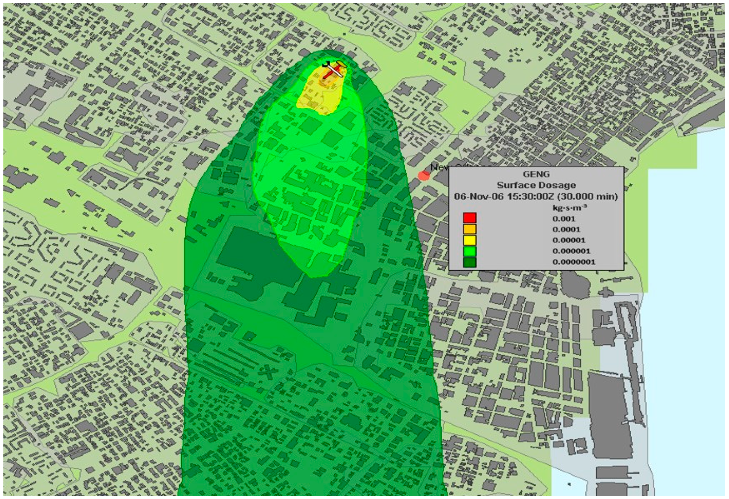Figure 1 shows an example output from UDM in which the evolution of the plume is affected by street alignment as well as building density, although the model is not resolving the dispersion around buildings. The principal outputs from Gaussian models are ensemble mean concentrations, but concentration fluctuations may also be provided through second order closure methods, such as that used in the second order integrated puff (SCIPUFF) code [6]. Nevertheless, the method has obvious limitations close to the source where the plume may have similar or smaller dimensions to the turbulence and obstacles. The former leads to highly stochastic dispersion, while the latter imposes and physical constraints on the transport and complex flow patterns. The assumption of Gaussian concentration distributions therefore breaks down at some point close to the source where concentration fluctuations and intermittency become important around obstacles.

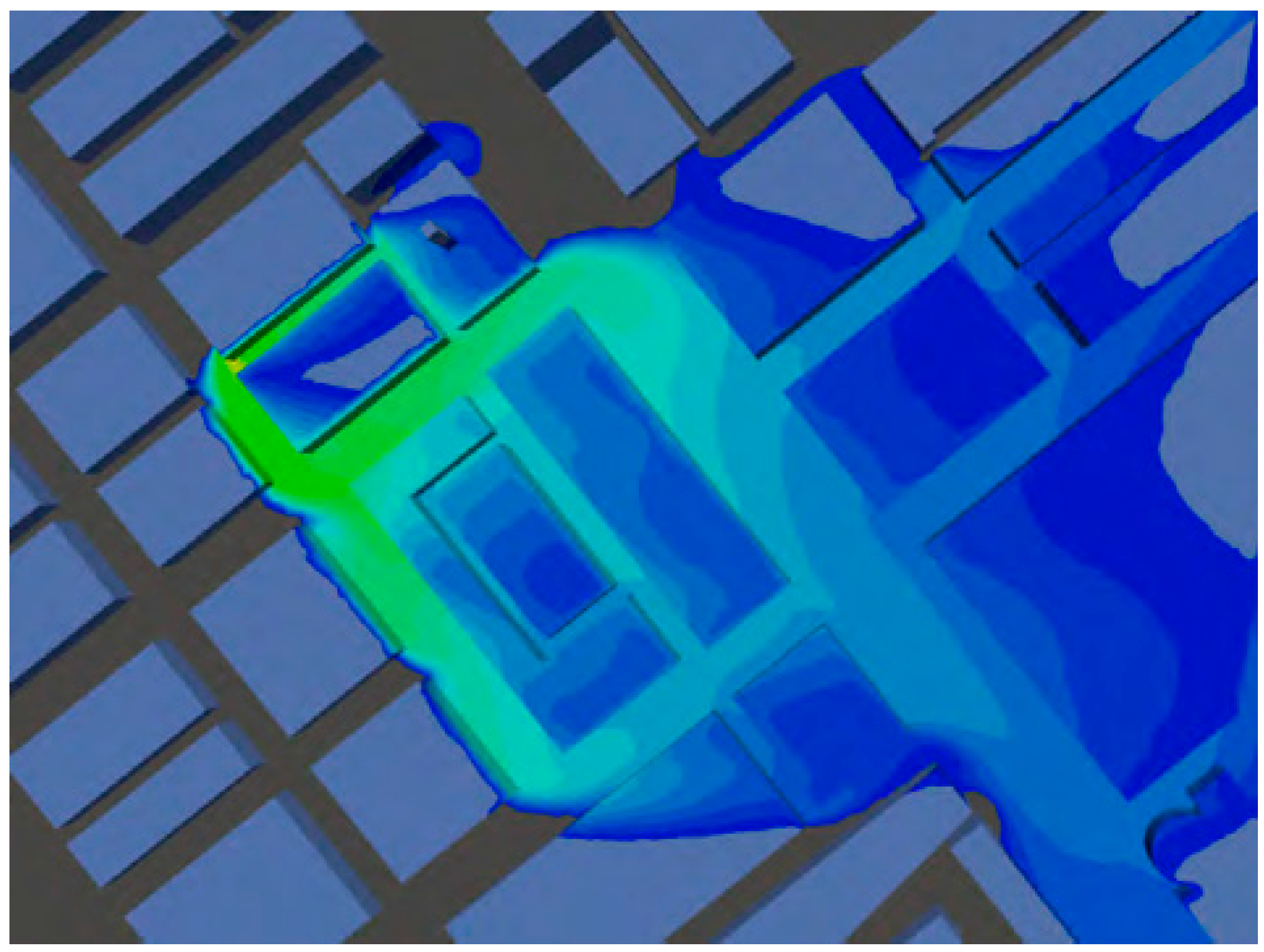
CFD methods resolve the dispersion around obstacles and two approaches are generally employed for AT&D simulations. The most commonly used solves the Reynolds Averaged Navier–Stokes (RANS) equations to calculate a steady wind field and leads to outputs that have some similarity to ensemble mean values. The second approach is termed large eddy simulation (LES). This solves the Navier–Stokes equations for the largest scales of turbulence (the effects of the unresolved small scales are parameterized) to provide high fidelity unsteady solutions for the concentration field around obstacles as shown in Figure 2. The dispersion of material into the streets surrounding the source illustrates the limitations of Gaussian concentration profile assumption in the near-field.

Although both RANS and the LES approaches appear innately superior to Gaussian methods, both rely on a series of modelling assumptions, commonly including the eddy-viscosity and gradient-diffusion hypotheses. The limitations of these approximations, even in the simplest flow fields, are well known and solutions are less accurate for low wind speed regions [8,9]. Britter and Hanna [10] have observed that although predictions from RANS methods may produce reasonable qualitative results for mean flows, their actual performance may be little better than that of simple Gaussian models when compared to experimental data. This means that CFD solutions cannot be said to have a known accuracy and can only be evaluated in relation to verification and validation benchmarks [9]. The pros and cons of Gaussian and CFD modelling approaches are summarised in

Table 1. The pros and cons of Gaussian and flow solution based atmospheric transport and dispersion (AT&D) simulation models.

Model Type	Pros	Cons	Examples
Gaussian	Simple inputs, rapid execution on PCs and laptops. Provide acceptable results for a wide range of releases.	May not resolve important details close to the source. Limited capability for resolving spatial and temporal variations in concentration.	UDM, SCIPUFF.
Flow solution	Provide detailed spatial and temporal predictions of hazard. Can handle all types of release.	Computational time and resources may be large compared to simpler methods. Complexity of solution process.	MicroSWIFT/SPRAY, RANS and LES.

.

The large range of AT&D models available is a reflection of the difficulty of accurately predicting how material will disperse in the atmosphere. Much of our understanding of the physics of atmospheric dispersion originates from studies of the dispersion of pollutants over open terrain conducted at Porton Down, Salisbury [11] where the mean height of the roughness elements, H, was much lower than the depth of the boundary layer, δ (i.e., H/δ << 1). In open terrain it is evident that material is likely to be rapidly dispersed by the sustained air flow aloft, but it is not clear how the physics of dispersion in open terrain translates to the very rough boundary layer flow over cities and urban areas [12,13,14]. In these, the scale of the roughness elements as characterised by the mean height of the buildings, may be a significant fraction of the height of the boundary layer depth, so that H/δ ~0.1.

Providing accurate predictions of dispersion in cities is particularly difficult because the local airflow is dependent on the geometry and arrangement of buildings and other structures as well as topography and complexities of the interaction with the flow aloft. These difficulties are compounded by temporal variations of wind strength and direction. Alas it is unlikely that errors will cancel. The extent to which physical understanding based on open terrain dispersion studies can be applied in urban environments is being further challenged by the trend towards developing central business districts (CBDs) composed of dense clusters of very tall office buildings in which H/δ may frequently exceed 0.1. For example, the La Défense area of Paris and the current developments in Melbourne shown in Figure 3 which illustrates the construction of a dense cluster of new 30-plus storey developments that dominate what were previously large buildings. There is little guidance on the physics that govern the characteristics of the complex boundary layers that develop over large cities and how they are modified by new large developments. Much remains to be learned about the fluid dynamical processes that control dispersion in such areas.

These gaps in understanding mean that modern AT&D models may model many physical processes through parameterisation. An example is the effect of stability on dispersion in urban environments. This leads to many competing parameterizations. The performance of a model is clearly enhanced by an effective parameterisation, but a growing problem is how to compare or assess the efficacy of complex numerical models that incorporate models of different processes and attendant parameterisations.

In practice, the accuracy of model predictions depends on the method used, the scenario to which it is applied, the input data available and the outputs that the user requires. Regardless of the AT&D model used it is essential that robust verification and performance evaluation procedures exist that are applicable to both open terrain and complex urban environments to ‘provide assurance of the robustness of predictions and to guide improvements in the modelling techniques’ [15].

3. Performance Metrics

A fundamental problem in evaluating AT&D models is that it is very difficult to encapsulate their performance in a single metric. This problem is exacerbated by the use of increasingly complex models for which the modelling of flow and dispersion should ideally be considered separately, and have different metrics. However, this is beyond the scope of the current review which is limited to considering the final dispersion prediction.

The difficulty of summarising AT&D model performance in a single metric leads most researchers to employ a range of statistical measures. These typically include, the normalized mean square error (NMSE), the fraction of predictions within a factor of 2 of the observations (FAC2), the fractional bias (FB), the geometric mean bias (MG) and the geometric variance (VG) (see Appendix A for definitions). In the absence of any universally agreed performance criteria, when authors wish to compare their results to those of others, they generally cite the criteria for an ‘acceptable model’ proposed by Chang and Hanna (e.g., [16,17,18,19,20,21,22]), which are summarized in

Table 2. The bounds of acceptable performance for dispersion models as proposed by Hanna et al. [21], Hanna and Chang [22] and Chang and Hanna [23].

Criterion	Rural	Urban
|FB|	<0.3	<0.67
NMSE	<3	<6
FAC2	>0.5	>0.3
NAD	<0.3	<0.5
MG	0.7 < MG < 1.3	-
VG	<1.6	-

. The Chang and Hanna criteria were based on their experience in conducting a large number of model evaluation exercises [23]. Examination of Table 2 shows that the urban criteria are relaxed by roughly a factor of two compared to rural ones ‘due to complexities introduced by buildings’ [24]. The metrics used by Chang and Hanna along with others have been adopted by HARMO, as part of a common model evaluation framework [25] through their incorporation into the BOOT statistical package [26].

While it is convenient to refer to the criteria in Table 2, it is important to note that (as detailed in [23]) they relate to comparisons made against ‘research-grade data’ for continuous releases. Where ‘research grade’ means experiments having on-site meteorology, a well-defined source term, high quality sampling, and ‘adequate’ quality assurance/quality control. Furthermore, it is assumed that the comparisons will relate to arc maximum concentrations (i.e., comparisons unpaired in space). This is important, as accurate evaluation of the arc maximum concentration and integrated cross-wind concentration are likely to be highly dependent on the spatial distribution of samplers (particularly in urban areas) as:

• The spatial resolution of the concentration measurements is likely to be relatively coarse;
• The maximum concentration value may not be well defined;
• The lateral extent of the plume may not be fully captured by the samplers;
• The crosswind-concentration measurements may well not be symmetrically distributed about the peak.

While the Chang and Hanna criteria provide a starting point, the caveats are quite restrictive and little guidance is provided as to the level of performance that should be expected when comparison data are paired in time and space, although it is stated that they should be relaxed ‘somewhat’ [23]. This is a critical question in relation to deciding if the metric is appropriate to the model application, such as determining if an AT&D model is suitable for use in emergency response scenarios, and understanding the benefits of using more sophisticated approaches. Furthermore, while the criteria may reveal important things about a model’s performance, they only provide a limited appreciation of model performance and little information regarding its strengths and weaknesses. For example,

Table 3. Statistical metrics for prediction from UDM compared against data for Prairie Grass release 49.

NMSE	FAC2	FB	MG	VG
0.09	0.58	−0.03	0.88	2.74

gives values for the metrics quoted above for a prediction from UDM compared to data for release 49 of the Prairie Grass experiment, which was a 10 min continuous open terrain release.

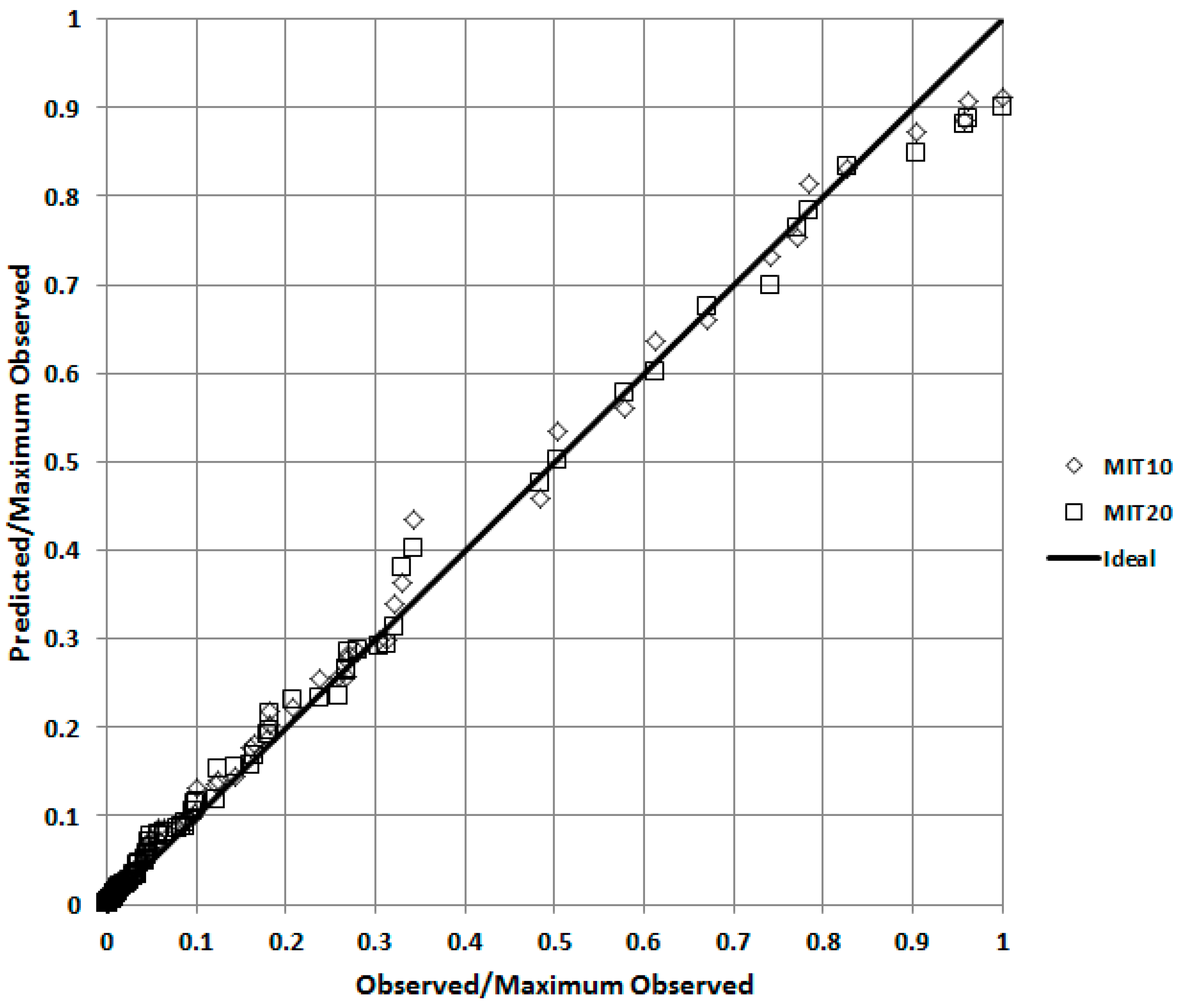
When compared to the values in Table 2 the model only satisfies four of the five criteria. More information is required to fully evaluate the model’s performance, and especially its spatial accuracy. A better appreciation of the model’s performance in a qualitative sense can be obtained by producing a quantile-quantile (QQ) plot, in which the predicted and observed concentrations are independently ranked and then plotted against each other. Figure 4 shows that UDM is generally predicting concentrations accurately over all distances, as the data points closely follow the diagonal line. The plot also shows that averaging the meteorological data over 10 or 20 min intervals (MIT10 and MIT20 respectively) has little effect on the results.

There is a large body of literature relating to the validation of CFD models in general, and a number of papers specifically related to validating CFD AT&D models, such as that by Schatzmann and Leitl [27], but no generally accepted standard. However, the Atomic Energy Society of Japan has developed a set of criteria for use in assessing CFD model predictions in comparison to wind tunnel data for neutral/slightly unstable conditions. These require FAC2 > 0.89 for ground level concentration along the plume axis, FAC2 > 0.54 for total spatial concentration, a correlation factor > 0.9 and a regression line slope of 0.9–1.1 [9]. The difference between these criteria and those in Table 2 suggest that there is no universal definition of acceptable model performance.

The difficulties associated with quantifying model performance in simple terms and the range of applications for AT&D models have led different researchers and organisations to develop their own preferred metrics on which they place particular emphasis. Examples include the 2-D measure of effectiveness (2-D MOE) and normalised absolute difference (NAD) developed by Warner et al. 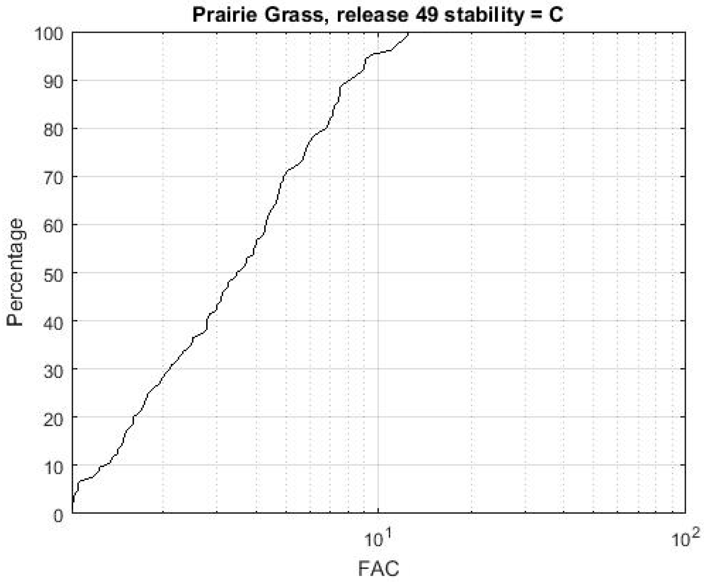[28] and the cumulative factor (CF) plot presented by Tull and Suden [29] (see Appendix A for details). A CF plot for UDM predictions compared to Prairie Grass release 49 is shown in Figure 5. This provides a good appreciation of how closely the predicted values match the observed ones, at the expense of any spatial information. It is worth noting that a number of automated tools have been developed to facilitate inter-model comparisons [30], but their use is generally limited to particular communities.

4. Data from Field Experiments

A good praxis for the evaluation of numerical models is to compare model predictions and field data, but in reality, this is difficult for a number of reasons. The first is that to conduct a field trial that provides research grade data involves deploying both a large amount of instrumentation and making a large number of releases. This is complex and costly, even for open terrain experiments, and these factors are compounded for measurement campaigns in urban areas. This led to a shortage of field data on the mean velocity field and scalar concentration field within cities (i.e., within the urban canopy) until relatively recently, and addressed by research on street canyons (e.g., [31]) and field campaigns in both Europe and the US, as summarised in

Table 4. Significant urban dispersion field experiments.

Town/City	Experiment	References
Basel	Basel UrBan Boundary Layer Experiment (BUBBLE)	[32]
London	Dispersion of Air Pollution and its Penetration into the Local Environment (DAPPLE)	[33]
Salt Lake City	Urban 2000	[34]
Los Angeles	Tracer Experiment	[35]
San Diego	Barrio Logan Experiment	[36]
Oklahoma City	Joint Urban 2004	[37,38]
Manhattan, NYC	Midtown	[38,39]

.

The data from these field campaigns has been invaluable, and enabled parameterisations to be developed for use in sophisticated AT&D numerical models. Nevertheless, the data captured is very limited in relation to the range of possible building configurations and the multiscale nature of the flow over such complex geometries. This can be appreciated by considering the range of locations in which cities exist, the degree to which they have been planned or developed organically; the range of architectural styles adopted; the presence of particular building types such as office blocks, shopping malls, warehouses, historic buildings, hospitals etc.

Although field trials may involve releases at different times during the day and night, and may be conducted over days or weeks, the range of meteorological conditions covered is inevitably quite limited. In addition, the characteristics of the local environment (such as surface roughness) are fixed by the location of the trial, while the amount of data obtained is governed by the numbers of sensors available, their spatial distribution and sampling periods. It is important to appreciate that even the biggest datasets acquired to date, such as those obtained in Project Prairie Grass and the Joint Urban 2003 (JU2003) experiment only contain a relatively small number of releases at a limited range of atmospheric conditions. A consequence of this is that they invariably represent only statistically small samples. This greatly restricts the degree of confidence that can be gained through comparing model predictions against a single data set. These issues are best appreciated by reference to a number of specific examples.

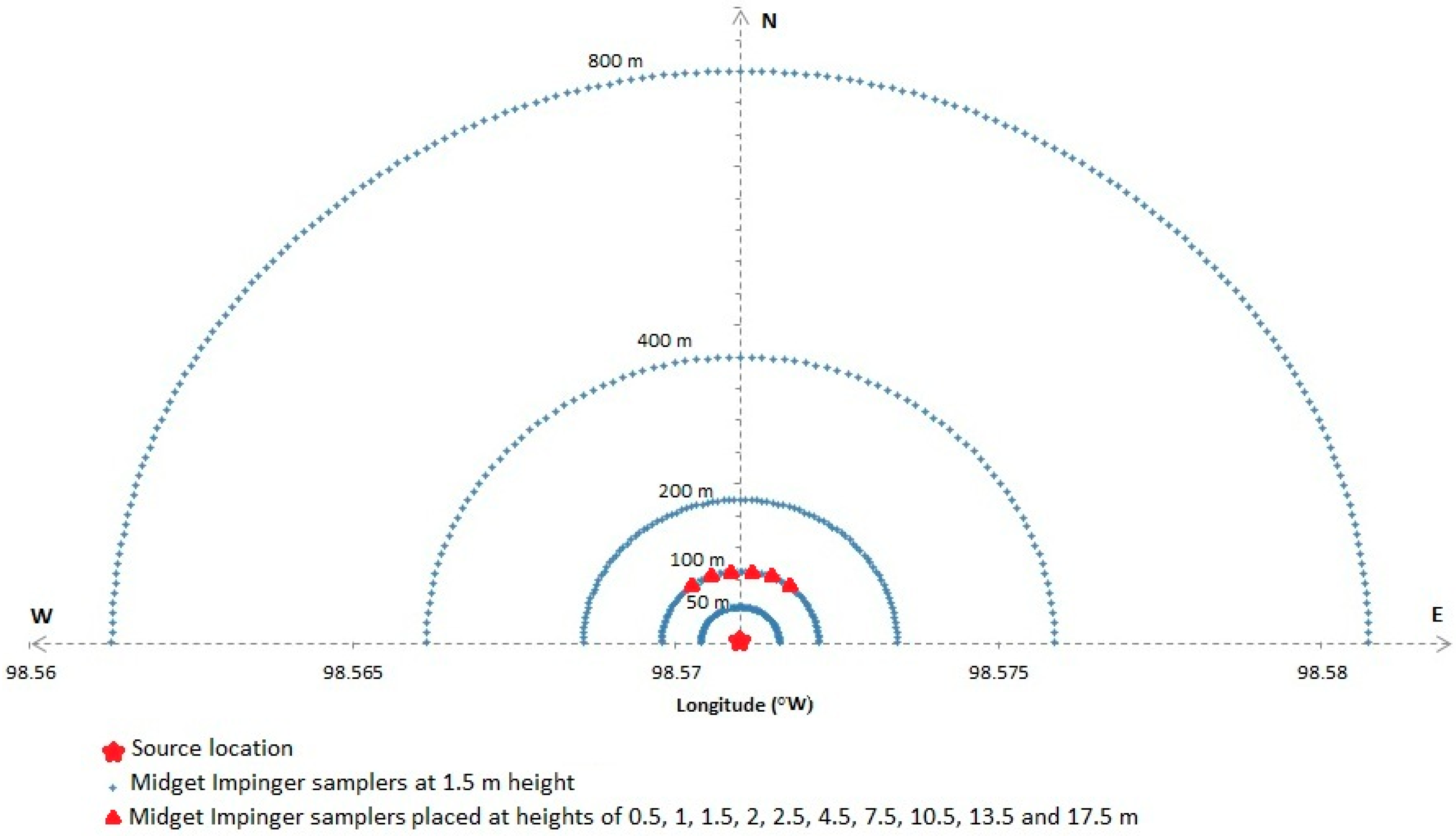
Probably the best known, and most analysed field dispersion dataset is that from the Project Prairie Grass (Haugen and Barad, [40]). In this experiment 600 samplers were deployed over a flat area of prairie in semi-circular arcs from 50–800 m to ensure that the plume was captured, as shown in Figure 6. This meant, however, that the number of samplers that recorded data (single concentration averages) was limited to a small fraction of the total number, so limiting the lateral definition of the plume; even so, the edges of a small number of releases were not fully captured. It can be seen from Figure 6 that the vast majority of samplers were at a height of 1.5 m, and that detailed vertical sampling at 10 heights was limited to a narrow sector of the 100 m arc close to the source. This is a limitation of most field experiments, in that although dispersion is a three-dimensional process, the sampler data is largely restricted to a single horizontal plane close to ground level, with only small numbers of measurements in the vertical dimension.

The Prairie Grass experiment consisted of 70 releases made close to the ground, each of 10 min duration, and meteorological data was recorded from a range of instruments around the sampler array. Examination of the trial reports ([40]) reveals that data from only 56 of the releases was considered usable. Furthermore, although the releases were made over a wide range of atmospheric stability conditions, 60% of the usable releases were made in neutral or slightly unstable conditions, with only very small numbers made at stable and very unstable conditions, as shown in

Table 5. Summary of Pasquill stability categories associated with usable data from the Prairie Grass releases.

Pasquill Stability Category	A	B	C	D	E	F
Number of releases	2	7	14	20	8	5

.

The Prairie Grass experiment shows that even in open terrain, the variability in dispersion means that a very large number of samplers are required to provide good spatial data coverage. If releases are made in an urban environment, in which material primarily disperses within the roughness layer characterised by a highly variable wind field, then an even greater number of samplers at a range of heights would be expected to obtain good coverage. However, as well as being prohibitively expensive, this is generally impractical due to constraints on where they may be placed.

JU2003 ([37,41]) is the best known large scale urban dispersion experiment. In thisa total of 130 samplers were deployed at ground level, plus a further 10 on the rooftops, within the Oklahoma City CBD and on three arcs at roughly 1, 2 and 4 km. Even so, the coverage was relatively sparse compared to the Prairie Grass experiment. The layout of the ground level samplers can be seen in Figure 7. The experiment comprised puff releases and 30 half hour releases made during 10 intensive operating periods (IOPs). The number of continuous releases for which usable data were recorded was 24, of which 12 were daytime releases and 12 night time. Although it is often assumed that stability conditions are neutral within cities, it is well-established that the JU2003 data indicate that significant differences in stability existed between the daytime and night time releases (e.g., [42]). If the stability conditions were constant for the day and night releases, then samples of 12 would not be very large, however, the assessment of model predictive accuracy using this dataset is further restricted by the fact that releases were made from three different locations.

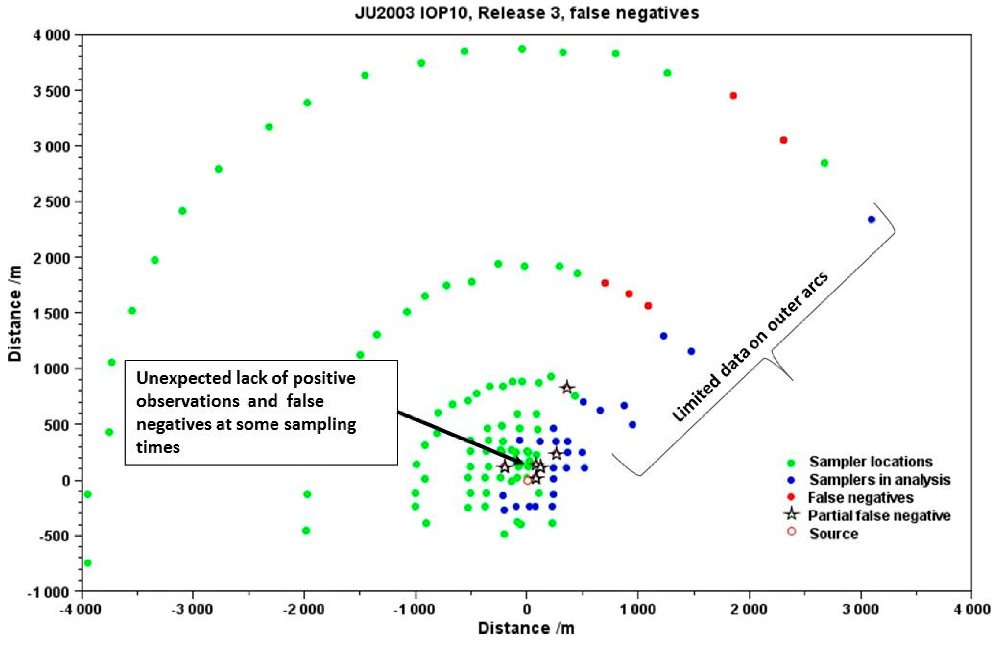
Figure 7 illustrates a comparison between a UDM prediction and sampler data for IOP 10 release 3 of JU2003. It shows a number of features, including how the majority of the samplers did not record any data; how the amount of data recorded on the outer arcs was very limited; and how due to the complexity of the urban environment some samplers that might have been expected to record data recorded nothing. Figure 7 also illustrates how the choice of meteorological input may affect the results of a comparison. In this case the input wind direction does not appear to be consistent with the actual measurements. This leads to a biased result with the predicted plume (blue dots) going outside the sampler array, and a string of false negative predictions (shown by the red dots). It is self-evident that the results of comparisons are highly dependent on the meteorological input provided to the model. Careful consideration must be given to deriving the most appropriate model input from the observed data. This should involve using multiple observations to support diagnostic wind field calculations, rather than for example basing dispersion predictions on a single (potentially unrepresentative) observation. Reducing uncertainty with respect to the meteorological input is critical to reducing uncertainty in the results of the comparison.

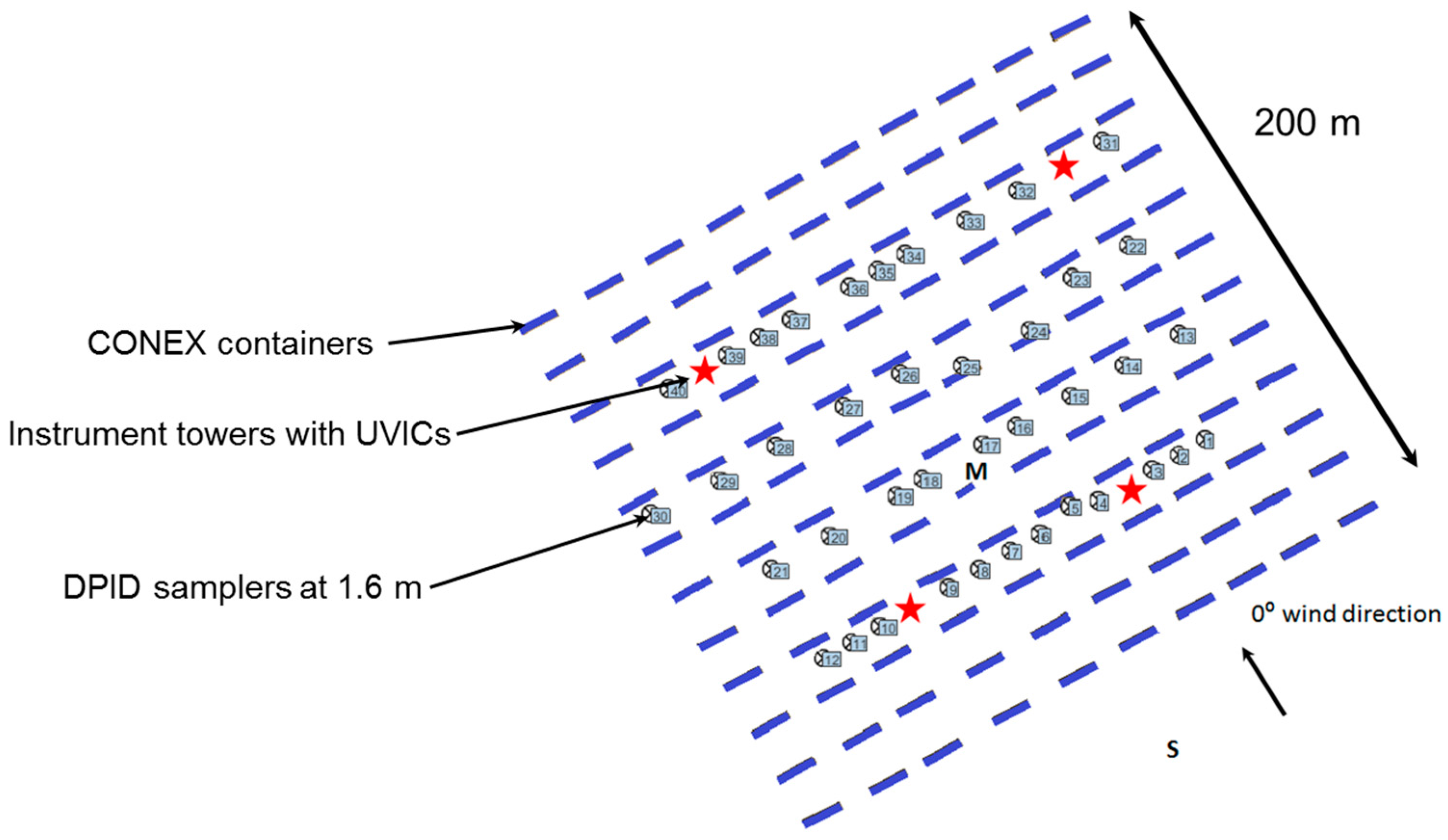
Figure 8 shows the layout of the mock urban setting test (MUST) [43,44]. In this experiment 120 CONEX containers were arranged in a regular grid over a 200 m square area, giving an array footprint area density of 8% (contrast this with the high density of buildings in central London shown in Figure 2). The sampling instrumentation consisted of 74 high frequency samplers. A total of 37 different release locations were used and 68 releases made with durations varying from 4 to 22 min. This multiplicity of variations makes identification of systematic errors between observed and predicted values difficult, although it is mitigated to a degree by the fact that the releases were made in the early morning and evening, which meant that the stability conditions were generally stable.

In addition to the very small sample sizes generally acquired, Tominaga and Stathopoulos [45] observe ‘the boundary conditions for field experiments are neither controllable nor repeatable’. They conclude that this constrains their usefulness for supporting systematic or parametric studies, which includes acquiring data against which to assess the performance of AT&D models. This is borne out by the above examples which relate to some of the most comprehensive datasets available, and suggests that comparisons against single data sets are not necessarily meaningful.

5. Data from Wind Tunnel Experiments

Some of the limitations of field experiments can be overcome by conducting wind (or water) tunnel experiments. These have the advantage of providing well-defined, constant, dispersion conditions that coupled with a reduction in scale support the acquisition of large data samples that enable comparisons to be made with a high degree of confidence [46]. They also have the advantage that sampling can be conducted at large numbers of locations and heights to provide good spatial coverage. Nevertheless, although considerable care may be taken to establish a boundary layer that accurately simulates real atmospheric conditions, the flow field in the wind tunnel cannot fully replicate that of the atmosphere, as the walls of the tunnel physically limit the maximum dimensions of the turbulence scales. In addition, although Reynolds number (Re) independent flows can be achieved for sharp-edged obstacles, Re effects may not be totally avoided for all geometries. Although the reduction in scale has the benefit of reducing the effective timescale, it also imposes limitations on the effective frequency of concentration fluctuations that can be measured. The reduction in scale also limits the detail that can be represented on models (e.g., roof top geometries are generally simplified and trees omitted). Although the effects of neglecting these are generally assessed as small, such assumptions nevertheless introduce uncertainties.

Wind tunnel experiments provide an important means of generating high quality, data at known conditions against which dispersion models may be compared, within certain constraints. The greatest restriction is in achieving similitude in cases where the thermal and buoyancy effects are significant [45]. This is because it is difficult to vary the stability conditions in a wind tunnel as the creation of thermally stratified flow fields requires heating and/or cooling, so creating and maintaining the desired boundary layer through the working section represents a considerable engineering challenge. This means that nearly all wind tunnel experiments are conducted in neutral stability conditions, despite the fact that stability effects significantly affect the atmospheric dispersion of material in open terrain and urban areas.

The model comparison exercise conducted against wind tunnel data in COST Action ES1006 (dispersion modelling for local-scale urban emergency response), showed that the values of performance metrics depended greatly on the choice of source and measurement locations [47]. This further illustrates the difficulty of understanding the absolute performance of a model.

6. Conducting a Model Comparison against Experimental Data

Section 3 highlighted the wide range of metrics used by researchers to describe the performance of AT&D models. In practice, the choice of metrics is driven by the context in which the model is to be used and sampler layout. The evaluation of long term air quality assessments may require arc maximum concentration values or integrated crosswind concentrations, the determination of which is consistent with the layout of the Prairie Grass experiment (Figure 6). The 2-D MOE is likely to be of greater interest for models used for short term emergency response modelling and its determination is consistent with the layout of the MUST experiment (Figure 8). In addition to the choice of metrics on which the evaluation is based, the analyst also makes a number of other important decisions regarding the basis on which the comparison is made, which may have a large impact on the results obtained. In particular they must choose:

• The degree to which the predictions and observations are spatially and temporally correlated;
• The criteria used for determining which data are included in the comparison.

If the data consists of a series of samples, then the first decision is to define the concentration averaging time over which the comparison is to be made. In the Prairie Grass experiment single 10 min samples were recorded for each release. However, in other experiments, such as JU2003 and MUST, multiple sequential samples were taken, enabling the concentration to be derived over a number of averaging times.

In general, performance metrics improve by adopting longer averaging times, as the importance of temporal correlation is reduced, while the adoption of spatial and temporal pair-wise comparisons is equivalent to imposing much more demanding performance requirements. The latter is perhaps more appropriate to AT&D models for emergency response, when accurate prediction of even short exposure times may be of concern. Good performance should therefore be expected for arc maximum comparisons in which spatial and temporal correlations are ignored.

In addition to the temporal and spatial averaging of data, the results of a comparison may be greatly affected by the data that are included or excluded from the comparison process. Initially, the analyst must determine which data are of sufficient quality (as indicated by a quality assurance flag) to be included in the analysis. Then they must define a zero threshold below which a sampler reading is taken to be zero. This must have a positive value to enable logarithmic parameters such as MG to be calculated, and should take into account any background concentration, the limit of detection (LOD) and limit of quantification (LOQ) of the samplers. The choice of zero threshold may have a large impact on the results if a large fraction of the concentration data have values close to it [23], depending on how the input data pairs are the filtered. The analyst has three options for filtering the observed and predicted data pairs [48]:

• Accept all;
• Accept if both above threshold;
• Accept if one above threshold.

It is important to note that the application of filtering strategies (2) or (3) leads to successively poorer performance metrics compared to strategy (1). A benefit of strategy (3) is that it reveals the presence of false positive and negative results that may be important when assessing AT&D models for emergency response.

The range of metrics, coupled with decisions described above regarding the degree of spatial and temporal correlation and filtering of data made in conducting AT&D model evaluations, make it difficult for a third party to assess how good a model is in absolute terms. This is further exacerbated by the effect of factors such as the choice of meteorological input and data fidelity. From this it is evident that any comparison should clearly state all the decisions made in conducting the comparison.

7. Making AT&D Model Performance More Transparent

In addition to comparisons with experimental data, a widely recognised approach to determining the efficacy of AT&D models is to conduct inter-model comparisons. This praxis alone is less robust than comparisons with field data, as the problem of determining the effectiveness of parameterizations of individual physical processes within a model cannot be addressed. However, comparisons with accepted models and field data promote a better overall understanding of performance. It is therefore suggested that comparisons between models and field data should also be presented alongside those for a standard reference model. This would have the advantage that performing a simultaneous field data and inter-model comparison would promote a more comprehensive overall evaluation and provide greater opportunities for diagnosing the strengths and weaknesses of different modelling approaches. Above all it would make model performance more transparent.

If it is accepted that performing comparisons against a standard reference model has utility, then its general adoption requires that its details are readily available, it is simple to implement and is applicable to a wide range of environmental conditions. In particular, it is necessary that such a model is able to provide predictions at a sufficiently good (i.e., practically useful) level of accuracy for a range of stabilities in open terrain and urban environments.

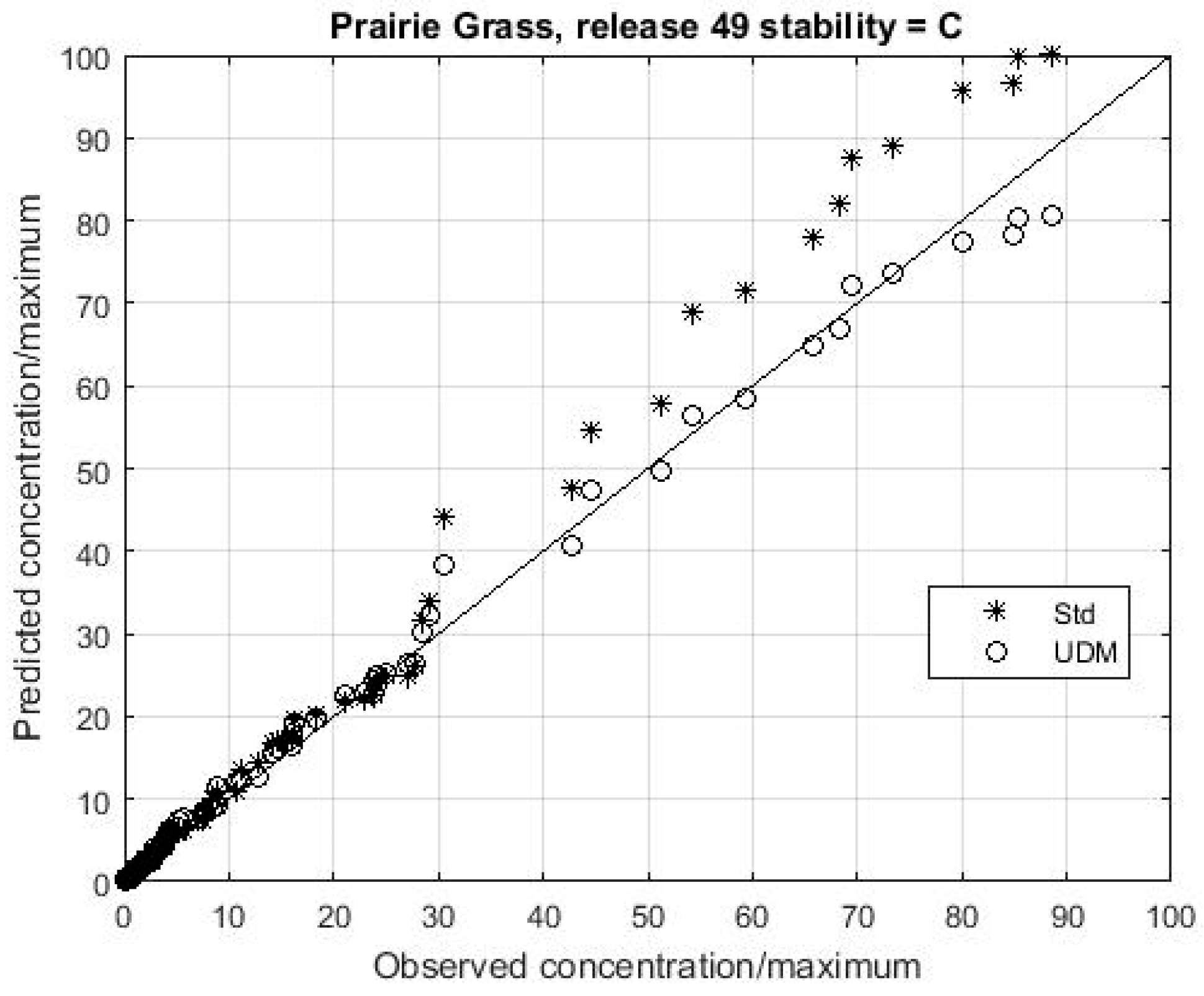
As a proof-of-concept an analytical Gaussian plume model for continuous ground level releases is taken which is applicable to open terrain and urban areas. The open terrain element of the proposed model is based on the work of Panofsky et al. [49] and Caughey et al. [50,51]. Figure 9 shows a QQ plot for Prairie Grass release 49 for the analytical model and compared to that from UDM (as shown in Figure 4). For this particular release, the plot shows that the analytical model provides similar predictions to UDM far away, but suggests that the more sophisticated relationships used in UDM (Similar to those used in the widely used US Environmental Protection Agency AERMOD code [36].) may provide better predictions close to the source.

The urban element is based on the analytical model developed by Franzese and Huq [52]. The model is based on a standard Gaussian formulation, in which the mean concentration c is predicted by Equation (1), in which y indicates the crosswind direction, z the vertical direction, ${\sigma }_y$ and ${\sigma }_z$ are the standard deviations of the crosswind and vertical distributions of concentration, respectively and $U$ is the reference wind speed and Q the mass release rate.

$$c=\frac{Q}{\pi U{\sigma }_y{\sigma }_z}\exp \left(-\frac{y^2}{2{\sigma }_y^2}-\frac{z^2}{2{\sigma }_z^2}\right)$$

(1)

In contrast to other simple urban dispersion models, which may be based solely on implementing empirical relationships derived from particular experiments (e.g., [53]), the model is derived from classical dispersion theory to provide a more general solution. The horizontal and vertical diffusion coefficients are determined according to the theories of Taylor [54] and Hunt and Weber [55] respectively as discussed in Franzese and Huq [52] (2011). The evolution of lateral and vertical spreads are calculated from the standard deviations of wind speed and length time scales appropriate to day and night conditions as detailed in Appendix B.

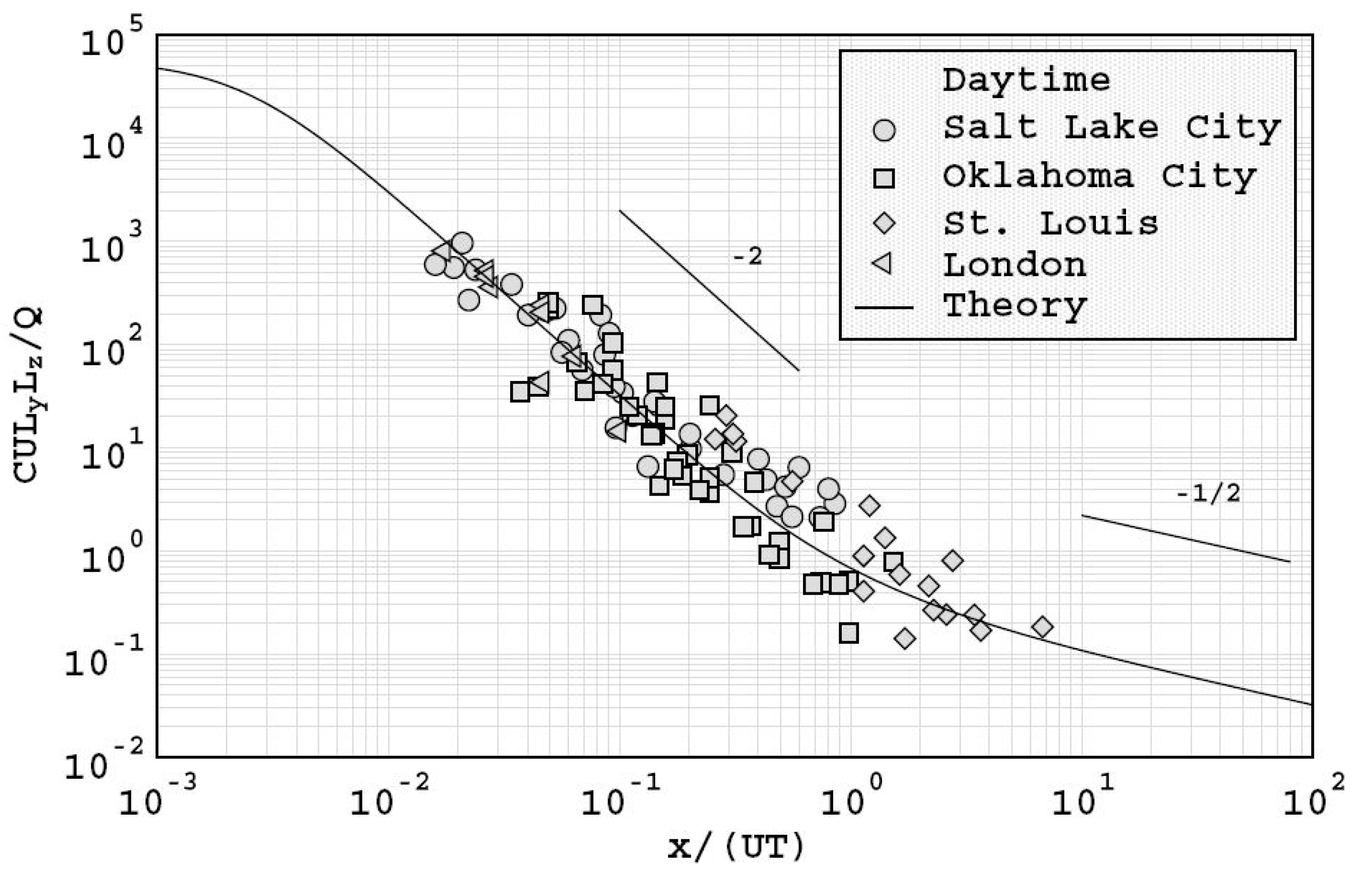
The comparisons conducted by Franzese and Huq [52] against data from urban experiments conducted in Oklahoma City, Salt Lake City, London, and St. Louis showed that the model predicted the existence of near and far field urban dispersion regimes. Their analysis showed that the dispersion process transitioned from a near-field regime to a far field regime at around $X/UT=10$ where $X$ is the downwind location, $U$ the mean wind speed at rooftop level and $T$ the square root of the product of the horizontal and vertical turbulence timescales. In addition, the results were consistent with the power law of the form $C\propto X^{-2}$, where $C$ is the maximum mean ground level concentration. This relationship has frequently been observed in urban experiments, and suggests that comparisons with field data may be undertaken using regressions of the form:

$$\frac{CU}{Q}=\frac{K_D}{X^2}$$

(2)

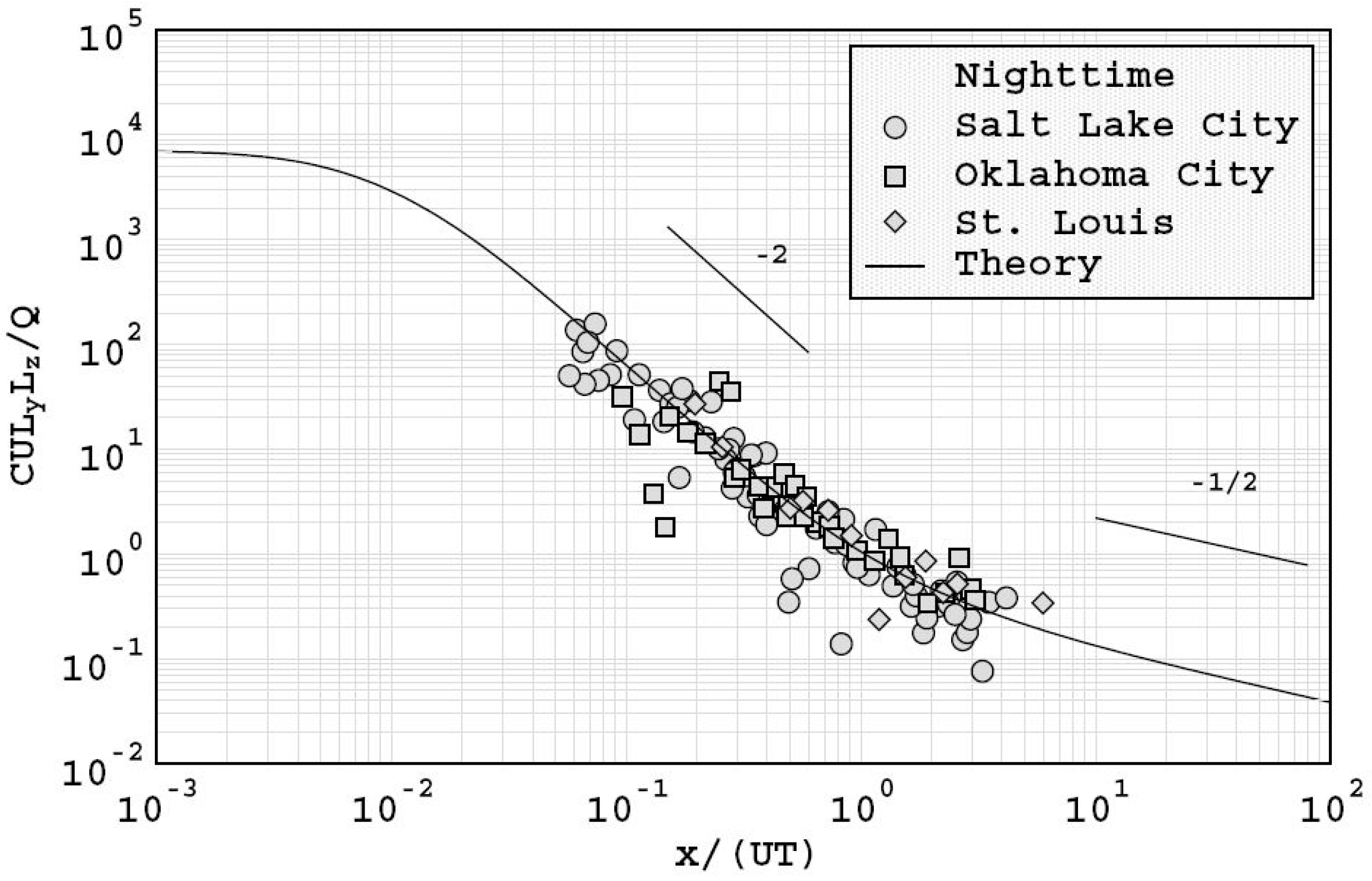
The work also suggested that urban dispersion was governed by the characteristic length scales of atmospheric boundary layer turbulence, rather than urban canopy length scales which were more likely to affect dispersion only in the vicinity of the source. The model predictions demonstrated a convincing collapse of data for both daytime conditions as shown in Figure 10, and night time conditions as shown in Figure 11, which indicate an ability to account for stability effects in urban areas.

The results shown in Figure 10 and Figure 11 indicate that although the model is simple, it accounts for a sufficient range of features that it provides a useful benchmark against which to assess the results from other urban dispersion models.

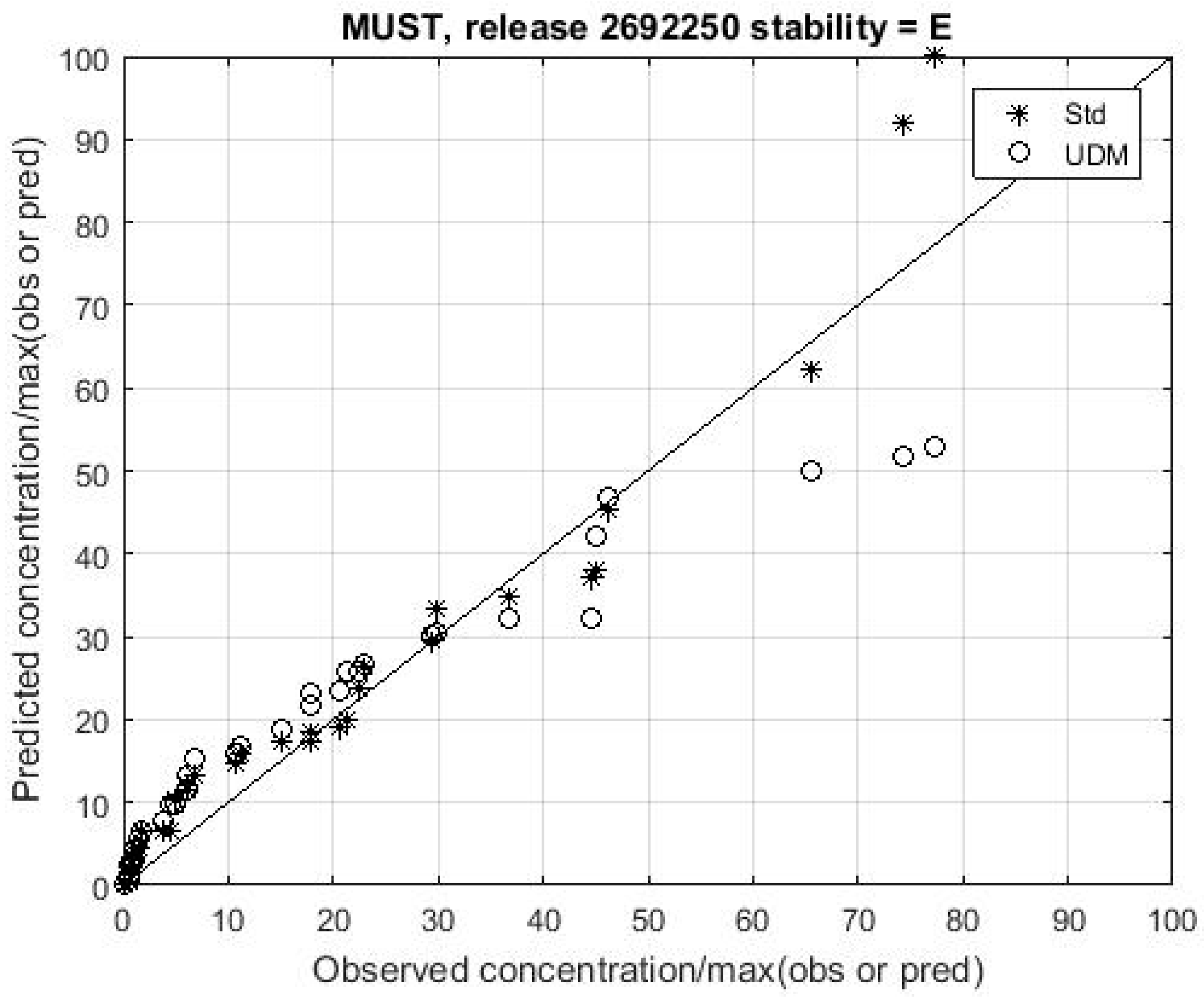
Figure 12 shows a QQ plot comparison of observations and predictions for UDM and the proposed reference model for a release in the MUST experiment. The model outputs are again quite similar except close to the source.

The results plotted in Figure 9, Figure 10, Figure 11 and Figure 12 show that a simple easily understood Gaussian plume model may provide predictions that are sufficiently accurate for it to serve as a useful reference model against which to assess the performance of all types of AT&D models for a wide range of environments and conditions, and particularly for quantifying the advantages of more sophisticated methods.

8. Conclusions

AT&D models of proven quality are required to support important decisions relating to air quality regulation, measures to improve air quality and emergency response actions following accidental or malicious releases of hazardous materials. At present, it is difficult for users to understand the relative accuracies of different AT&D models, and hence to ascertain the benefits of utilizing different or more sophisticated models.

Examination of the literature has shown that a range of metrics are adopted to evaluate the performance of AT&D models, but the only quantitative performance acceptance criteria generally referred to are those proposed by Chang and Hanna. However, those criteria are based on a limited number of metrics and are subject to number of important conditions. It is not clear how the acceptance criteria should be modified when the specified conditions are not met, and related to such factors as the concentration averaging time.

Examination of the data available from even the largest open terrain and urban field experiments has shown that the number of releases conducted under even nominally similar conditions is invariably too small to be statistically robust. Furthermore, in comparison to the spatial volume of interest, the data is relatively sparse and generally limited to a plane close to the ground. The sample size and repeatability limitations of field experiments may be mitigated to a degree by using data from wind tunnel experiments, but significant limitations remain in the extent to which atmospheric stability and turbulence spectra can be represented. The net result is that model comparisons against field and wind tunnel data may only give a limited understanding of performance.

Whatever the source of experimental data, decisions relating to the inclusion or exclusion of data, definition of effective zero concentration values and filtering of data mean that without access to full details of a comparison, it is extremely difficult for a third party to fully appreciate how good a model is. This issue may be alleviated to the benefit of the whole community by encouraging researchers to adopt a common process, and include a comparison against a reference model, which supports an assessment of model strengths and weaknesses and the effectiveness of competing parametrisations.

As a proof-of-principle a simple analytic Gaussian reference model suitable for simulating dispersion from ground level continuous releases in open terrain or urban environments has been defined. This model is based on the urban dispersion model developed by Franzese and Huq [52], but includes relationships derived by Panofsky et al. [49] and Caughey et al. [50,51] to predict open terrain dispersion. Use of this model has been demonstrated in assessing predictions from the UDM against data from the Prairie Grass and MUST experiments.

Based the results obtained, the authors believe that use of a reference model should be an integral component of the evaluation protocol.