A Vortex-Induced Correction Method for Pressure Loss Prediction in Fluid Network Theory

Abstract

Traditional fluid network theory often underestimates pressure losses in complex pipe-bundle systems operating under vortex-dominated flow conditions, with deviations exceeding 20% in many cases. To address this limitation, this study proposes a vortex-based correction method. Three-dimensional simulations were performed on a multidirectional parallel pipe bundle to analyze vortex formation and to quantify the effects of fluid properties (viscosity and inlet velocity) and structural parameters (branch diameter, manifold cross-sectional ratio, and manifold arrangement) on pressure loss. To account for vortex-induced energy dissipation that is overlooked by conventional one-dimensional network models, an additional vortex-induced loss coefficient, α, is introduced to modify the pressure-loss formulation. Results indicate that higher viscosity, larger branch diameter, a higher manifold cross-sectional ratio, and a co-flow arrangement improve flow uniformity and prediction accuracy. Conversely, higher inlet velocities and counter-flow arrangements intensify vortex effects and increase prediction deviations. Least-squares fitting indicates that α ranges from 1.15 to 1.37. Implementation of the proposed correction reduces pressure-loss prediction errors to within 5%, demonstrating the method’s effectiveness and extending the applicability of fluid network theory to vortex-dominated flows.

1. Introduction

Fluid network theory serves as a fundamental framework for predicting fluid behavior and pressure losses in complex piping systems. It has been widely used in engineering practice, fluid mechanics research, and the design of thermal-energy systems. By modeling a piping system as a network of one-dimensional flow elements and applying the governing equations of mass and energy conservation, this theory enables rapid estimation of pressure distributions and flow-rate allocation, offering high computational efficiency and practical value for engineering applications [1]. At high Reynolds numbers, turbulence and inertial effects intensify three-dimensional separation and mixing, making pressure-loss prediction increasingly sensitive to local flow structures [2]. However, in pipe networks with complex geometries, traditional theory often underestimates pressure losses, leading to errors exceeding 20% in some cases [3].

Recent advances in computational fluid dynamics (CFD) have enabled more detailed characterization of local flow structures and energy dissipation mechanisms. Previous studies have established quantitative links between vortex structures in sudden-expansion regions and their corresponding pressure-loss coefficients, providing a basis for refining resistance models in fluid network theory. The incorporation of additional loss terms or the adoption of resistance models derived from CFD and experimental data can significantly enhance pressure-loss predictions, thereby providing more reliable support for engineering design [4]. For example, Gao et al. [5] proposed a corrected pressure-loss model based on particle-flow and one-dimensional flow theories, substantially reducing the deviation between predictions and experimental data. Li et al. [6] conducted systematic experimental and numerical investigations of variations in local resistance coefficients under contraction–expansion geometries and varying flow conditions, subsequently developing updated quantitative models for local-loss correction. Driven by the development and validation of these approaches, research regarding pressure-loss mechanisms and corresponding correction methods in fluid networks has expanded rapidly. Collectively, these advances have facilitated the application of fluid network theory to pipe networks characterized by pronounced vortex effects and complex geometries.

Pressure losses in complex piping systems primarily arise from vortex generation and flow separation, which inevitably lead to energy dissipation. These inherently three-dimensional phenomena play crucial roles in determining energy efficiency and flow uniformity.

Local resistance coefficients depend heavily on the geometry of pipe fittings. Moreover, vortex formation and recirculation induced by sudden expansions, elbows, and branching structures can result in substantial additional energy losses [7]. Numerous studies [8] indicate that rapid and accurate pressure-loss prediction relies not only on empirical correlations but also on refined analysis and correction methods that integrate CFD simulations and experimental data to capture flow complexity and nonlinear effects. For instance, M et al. [9] investigated flow resistance in trifurcation pipe networks, demonstrating that complex branching substantially increases resistance; accordingly, they proposed an optimization strategy to reduce pressure losses. He et al. [10] analyzed vortex-induced turbulent flow in urban stormwater manholes using CFD, revealing that vortex-driven turbulence significantly impacts flow stability and energy dissipation. Thorat et al. [11] examined the relationship between major and minor losses in pipeline systems and proposed optimization strategies to improve energy efficiency. Zhang et al. [12] conducted three-dimensional CFD simulations to investigate turbulent flow and pressure characteristics in circular elbows with varying bend angles. They reported a non-monotonic trend where, as the bend angle increases, the overall pressure loss first increases, then decreases, and finally increases again. Notably, as the bend angle approaches 90°, strong secondary flow effects induce the maximum pressure loss. Yao et al. [13] conducted CFD analyses of turbulent flow in pipes with sudden expansions and recirculation regions, finding that sudden-expansion zones significantly affect pressure drop, with recirculation further intensifying overall energy dissipation. Review studies [14,15] further indicate that, facilitated by continuous improvements in computational capability, validated CFD has become an essential tool for investigating complex flow behavior and pressure-loss mechanisms. Detailed flow-field information can subsequently be used to refine empirical correlations for engineering design. Regarding manifold-type distributing devices and branched pipe networks, numerical studies [16,17] have shown that structural parameters—such as bend radius, branching angle, and branch diameter—significantly influence flow uniformity and resistance distribution. This suggests that geometric optimization is a practical approach to reducing energy losses. More recently, machine learning techniques have been integrated with CFD or experimental data to develop regression-based models. These models enable more efficient prediction of pressure drop and resistance characteristics, while facilitating the optimization of pipe components and network layouts [18]. In light of these advances and practical needs, improving numerical simulation strategies, correcting traditional pressure-loss models, and integrating large-scale CFD data with empirical calibration have emerged as key directions for enhancing prediction accuracy and engineering applicability in complex pipe networks.

The present study aims to improve pressure-loss prediction in parallel-pipe molten-salt systems. By integrating CFD simulations with fluid network theory, this work systematically investigates the effects of fluid properties and structural parameters on pressure loss and prediction accuracy. A vortex-based correction method is proposed, introducing an additional loss coefficient, α, to modify the conventional resistance model. The corrected model is subsequently validated to demonstrate its effectiveness and engineering applicability.

In contrast to existing CFD-based correction approaches that rely on case-specific resistance coefficients, the proposed method introduces a vortex-induced additional loss coefficient that can be directly embedded into conventional fluid network solvers. This approach preserves the computational efficiency of traditional fluid network theory while significantly enhancing the accuracy of pressure-loss predictions.

2. Methods

2.1. Physical Model Construction

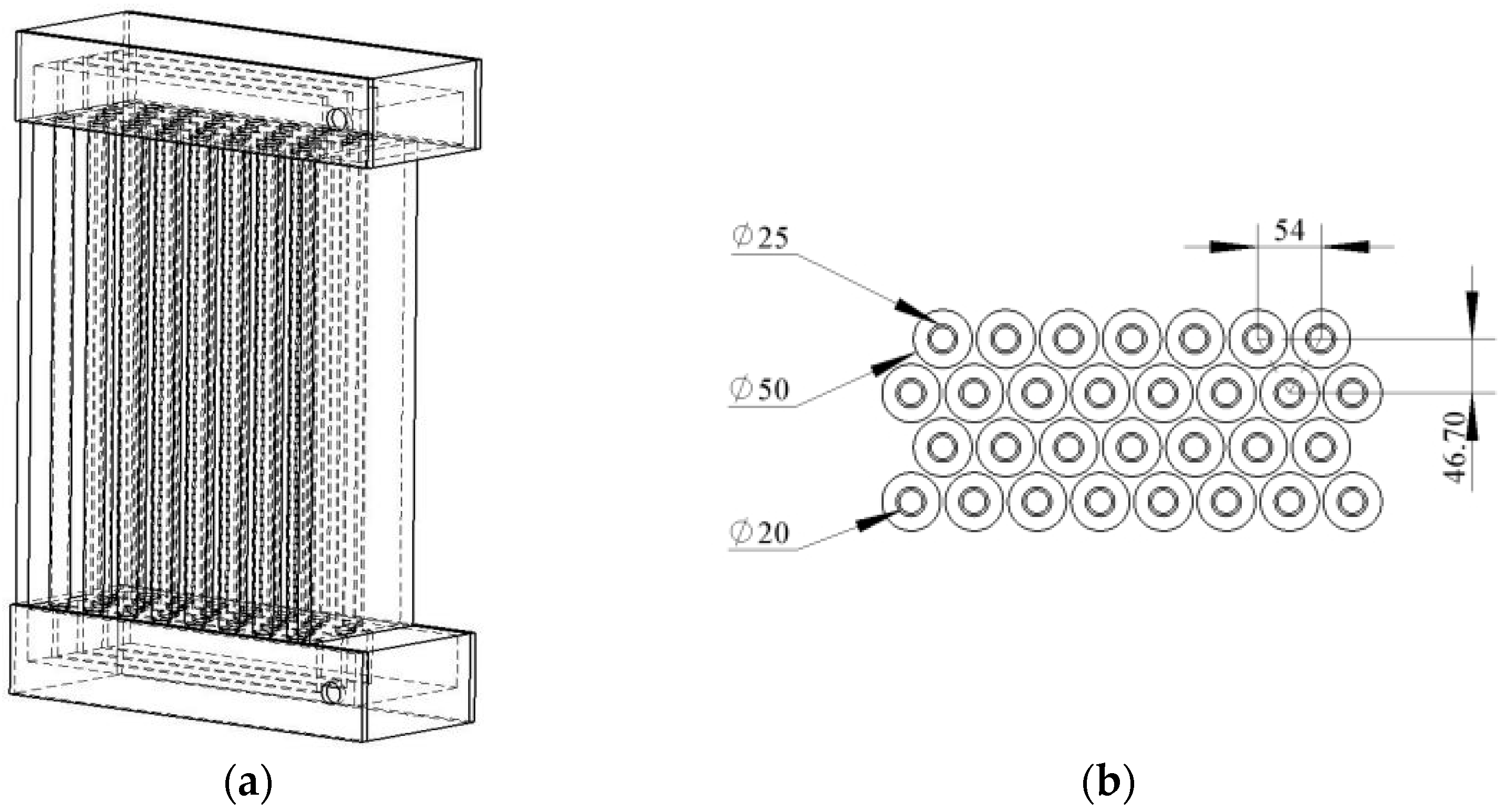
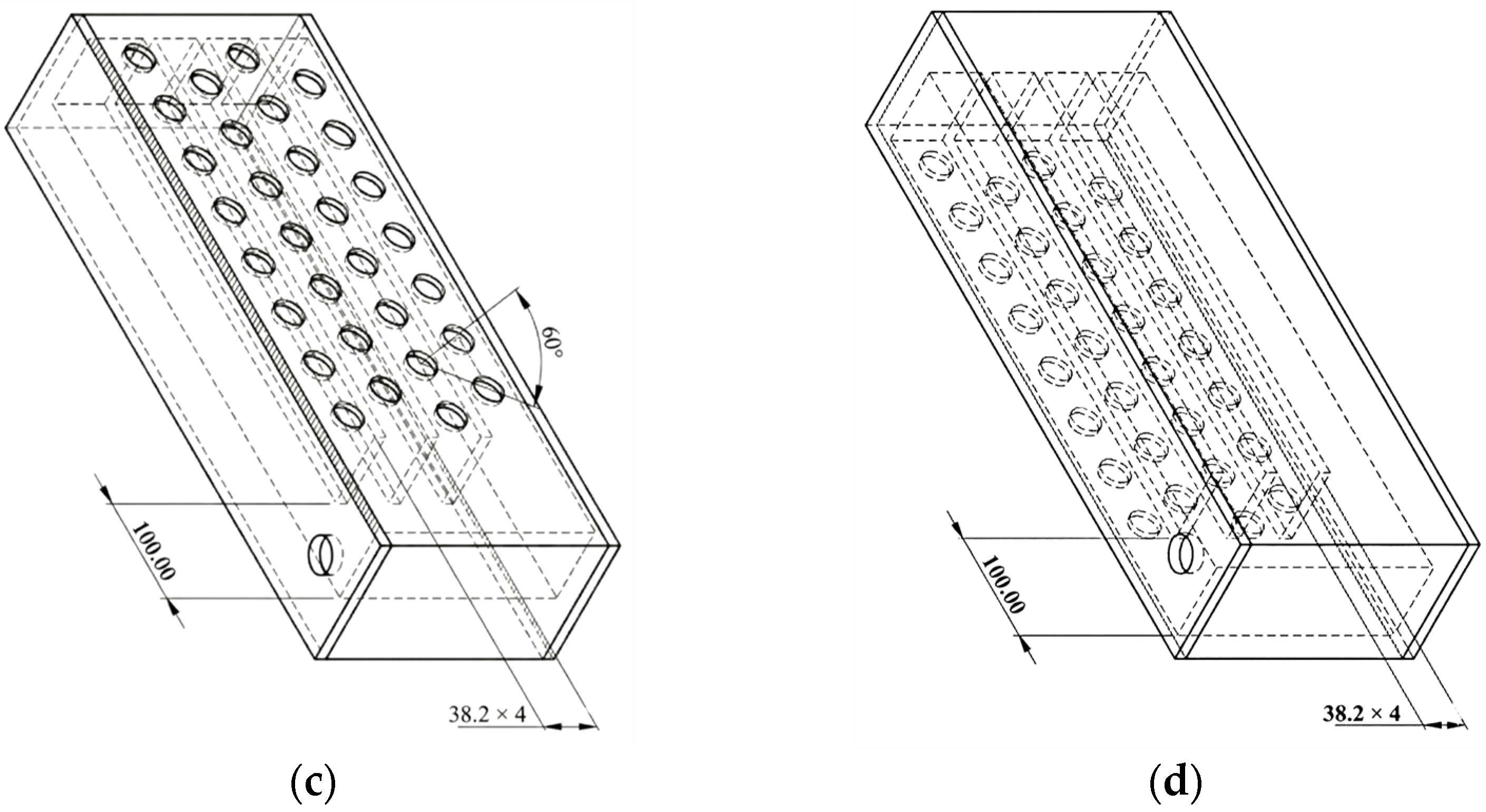
The physical model considered in this study is a parallel pipe bundle used in a molten-salt heat exchanger. The system consists of three main components: a distribution manifold, parallel finned-tube bundles, and a collection manifold, as shown in Figure 1. Molten salt enters the distribution manifold through the inlet and is subsequently divided among the parallel branch pipes. The streams are then recombined in the collection manifold and discharged through the outlet.

In the parallel pipe bundle, each finned-tube channel has a 20 mm diameter. The transverse and longitudinal pitches are 54 mm and 46.7 mm, respectively. Both the inlet and outlet pipes have a diameter of 30 mm. Throughout the system, the molten salt flows upward. This configuration is widely used in practice and helps improve the uniformity of flow distribution among parallel branches.

2.2. Fluid Network Theory Model

2.2.1. Pressure Loss Formulation

Throughout this study, pressure loss is consistently expressed in terms of pressure loss (Pa), and frictional losses are evaluated using the Darcy–Weisbach formulation with the Darcy friction factor $f$. Based on fundamental fluid mechanics principles, the molten-salt flow within the parallel pipe bundle may be classified as laminar or turbulent, depending on the Reynolds number. Accordingly, the flow regime is characterized by the Reynolds number Re, as defined in Equation (1).

$$Re={\displaystyle \frac{\rho vD}{\mu }}$$

(1)

where $Re$ is the Reynolds number; $v$ is the fluid velocity (m·s⁻¹); $\rho$ is the fluid density (kg·m⁻³); $D$ is the pipe diameter (m); and $\mu$ is the dynamic viscosity (Pa·s).

Based on the overall structure of the heat exchanger, the parallel pipe bundle can be simplified as a fluid network theory model consisting of a distribution manifold, parallel branch pipes, and a collection manifold.

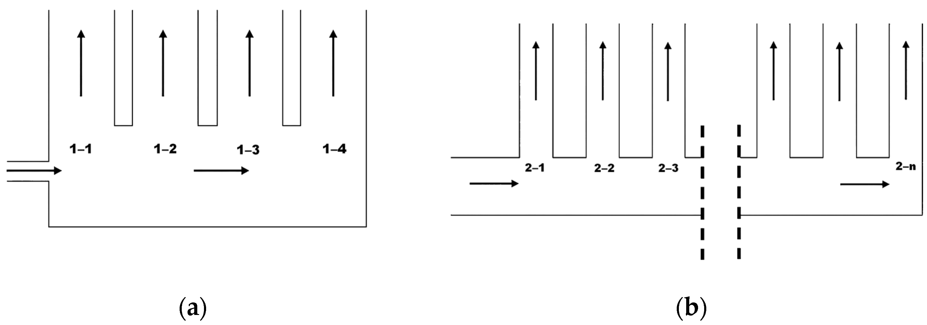
The model describes flow-rate distribution and pressure-loss characteristics using continuity and energy-conservation equations. A schematic of the flow in the distribution manifold is shown in Figure 2.

For a constant-cross-section distribution manifold, the energy–conservation relationship between Sections 1–1 and n–n can be expressed as follows.

$$P_{f1}+{\displaystyle \frac{\rho V_{f1}^2}{2}}=P_{fn}+{\displaystyle \frac{\rho V_{fn}^2}{2}}+\sum _{i=1}^n∆P_{f1}$$

(2)

where $P_{f1}$ is static pressure at section 1–1 of the header (Pa); $P_{fn}$ is static pressure at section n–n of the header (Pa); $V_{f1}$ is axial velocity at section 1–1 of the header (m s⁻¹); $V_{fn}$ is axial velocity at section n–n of the header (m s⁻¹); $\sum _{i=1}^n∆P_{f1}$ is total pressure loss due to frictional and local resistances between sections 1–1 and n–n (Pa).

From Equation (2), the static pressure at section n–n can be derived as shown in Equation (3).

$$∆p_{f1-n}=P_{fn}-P_{f1}={\displaystyle \frac{\rho \left(V_{f1}^2-V_{fn}^2\right)}{2}}-\sum _{i=1}^n∆P_{fn}$$

(3)

where ${\displaystyle \frac{\rho \left(V_{f1}^2-V_{fn}^2\right)}{2}}$ is the dynamic pressure difference between the two sections in the axial channel (Pa).

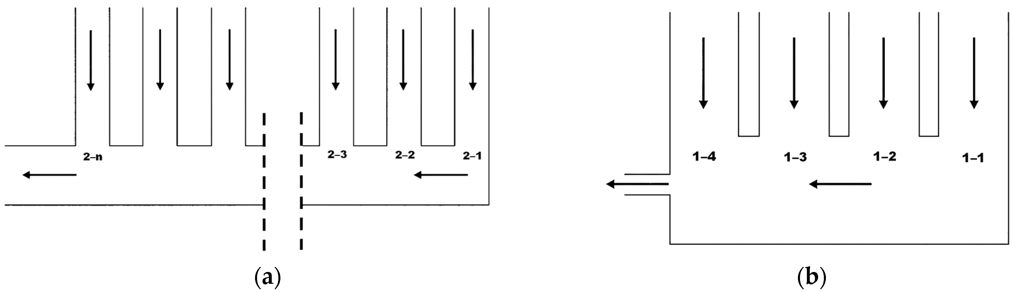
A schematic of the flow in the collection manifold is shown in Figure 3.

For the collection manifold, the static-pressure variation can be expressed as Equation (4):

$$∆P_{h1-n}=P_{hn}-P_{h1}={\displaystyle \frac{\rho }{2}}\left(V_{h1}^2-V_{hn}^2\right)-\sum _{i=1}^n(∆P_{ht})$$

(4)

Because frictional and local losses accumulate along the flow path, the static pressure in the outlet manifold decreases monotonically in the flow direction.

For each branch pipe, the inlet–outlet pressure difference can be expressed as Equation (5):

$$∆P_n=P_{fn}-P_{hn}=\rho g(h_h-h_f)$$

(5)

where $∆P_n$ is the pressure difference between the inlet and outlet of a branch pipe in the parallel pipe group (Pa); $P_{fn}$ is the static pressure at the inlet of the branch pipe in the parallel pipe group (Pa); $P_{hn}$ is the static pressure at the outlet of the branch pipe in the parallel pipe group (Pa); $g$ is the gravitational acceleration (m s⁻²); $h_h$ is the elevation of the outlet header (m); $h_f$ is the elevation of the inlet header (m).

When the inlet and outlet manifolds are located at the same elevation (i.e., h_in = h_out), the inlet–outlet pressure difference in the parallel branch pipes can be further simplified, as shown in Equation (6).

$$∆P_n=P_{fn}-P_{hn}=\rho \xi {\displaystyle \frac{V_n^2}{2}}$$

(6)

where $V_n^2$ is the fluid velocity inside the branch pipe of the parallel pipe group (m s⁻¹). $\xi$ is the total resistance coefficient of the parallel branch pipe (dimensionless).

From the above relationships, uniform flow distribution among parallel branches requires the inlet and outlet static pressures of each branch to be approximately equal. That is, the static-pressure distributions in both the inlet and outlet manifolds should be as uniform as possible.

2.2.2. Pressure Loss Model of the Parallel Pipe Bundle Based on Fluid Network Theory

In the fluid network model of the parallel pipe bundle, the total pressure loss is determined by continuity and energy conservation. It consists of frictional losses along the manifolds and branch pipes, as well as local losses at the manifold–branch junctions, as expressed in Equation (7).

$$\Delta P_{total}=P_{IN}-P_{OUT}=\Delta P_f+\Delta P_m$$

(7)

where $P_{IN}$ is inlet pressure of the parallel pipe bundle (Pa); $P_{OUT}$ is outlet pressure of the parallel pipe bundle (Pa); $\Delta P_f$ is pressure loss along the route (Pa); $\Delta P_m$ is local pressure loss (Pa).

The total pressure loss across the parallel pipe bundle arises from both distributed frictional losses and local losses associated with flow splitting, merging, and geometric discontinuities. Under a consistent sign convention, these losses are additive. In practical parallel pipe bundles, the pressure loss is primarily governed by frictional effects in the branch pipes and manifolds. Therefore, a unified frictional pressure-loss formulation applicable to both laminar and turbulent flow regimes is adopted, as expressed in Equation (8).

$$\Delta P=f{\displaystyle \frac{l}{D}}{\displaystyle \frac{\rho u^2}{2}}$$

(8)

where $f$ is the Darcy friction factor. The value of $f$ depends on the flow regime, which is characterized by the Reynolds number; $l$ is the length of the flow pipeline (m); $D$ is the diameter of the flow pipeline (m); $\rho$ is the fluid density; and $u$ is the mean flow velocity (m s⁻¹); $\Delta P$ denotes the pressure loss (Pa).

For laminar flow (Re < 2000), the Darcy friction factor is computed from laminar pipe-flow theory, as given in Equation (9).

$$f={\displaystyle \frac{64}{Re}}$$

(9)

Substituting this relation into the Darcy–Weisbach equation yields the classical Louisville pressure-loss expression for laminar flow.

$$\Delta p_L={\displaystyle \frac{32\mu lv}{D^2}}$$

(10)

where $\Delta p_L$ is the pressure loss due to laminar flow (Pa).

For turbulent flow, the friction factor is calculated using an empirical correlation, as given in Equation (11).

$$f={\displaystyle \frac{0.3164}{{Re}^{1/4}}}$$

(11)

where $f$ is the friction factor for turbulent flow.

Substitution of the Blasius correlation into the Darcy–Weisbach equation gives the turbulent-flow pressure-loss formulation used in this study. Because the pipe walls are assumed hydraulically smooth in this study, the Blasius correlation is adopted for smooth turbulent pipe flow within its customary applicability range (typically 4 × 10⁻³ ≤ Re ≤ 10⁻⁵). Accordingly, wall-roughness effects are neglected.

$$\Delta P=0.3165{\displaystyle \frac{L}{D}}{\displaystyle \frac{\rho u^2}{2}}{\left({\displaystyle \frac{\rho vD}{\mu }}\right)}^{-1/4}$$

(12)

In the parallel pipe bundle, high-viscosity molten salt flows through constant-cross-section distribution and collection manifolds, with flow splitting and merging occurring through the longitudinal branch pipes. Because the flow rate varies along the flow direction, the mean Reynolds number and the friction factor in the manifolds vary accordingly.

2.3. Basic Assumptions and Boundary Condition Settings

To characterize the flow behavior and pressure-loss characteristics of molten salt in the parallel pipe bundle, a three-dimensional steady-state numerical model was developed. The simulations were performed under the following assumptions.

• Molten salt was modeled as an incompressible Newtonian fluid.
• The flow was assumed to be three-dimensional and steady.
• Phase change and chemical reactions were neglected.
• The pipe walls were assumed to be rigid and hydraulically smooth, and the influence of wall roughness on the flow was neglected.
• Since the inlet and outlet of the system were located at the same elevation, the effect of gravity on pressure loss was neglected in this study.

In the numerical simulations, molten salt was adopted as the working fluid and modeled as an incompressible Newtonian fluid. A velocity-inlet boundary condition was imposed at the inlet, while a pressure-outlet boundary condition was specified at the outlet. All solid walls were treated as no-slip boundaries. Turbulence was modeled using the realizable k–ε model with enhanced wall treatment, selected for its robustness in complex internal flows and proven capability to predict flow separation and rotational flow in manifold systems. Compared with the standard k–ε model, this approach provides improved accuracy while maintaining reasonable computational cost. Enhanced wall functions were employed to accurately resolve near-wall turbulent behavior without excessive mesh refinement.

The governing equations were discretized using the finite-volume method, and pressure–velocity coupling was handled using the SIMPLE algorithm. The momentum and turbulence equations were discretized using second-order upwind schemes to improve numerical accuracy. Steady-state simulations were performed, and convergence was assumed when the residuals of the continuity, momentum, and turbulence equations decreased below 10⁻⁴ and the monitored inlet–outlet pressure loss varied by less than 0.5%.

2.4. Mesh Generation and Grid Independence Verification

Due to the geometric complexity of the parallel pipe bundle, the computational mesh was generated using the ANSYS Workbench (2022) mesh module. An unstructured tetrahedral mesh was employed throughout the computational domain, with local refinement applied in key flow regions—including the distribution manifold, the collection manifold, and the branch–manifold junctions—to improve the resolution of complex flow structures. The base mesh size was set to 4 mm, resulting in approximately 8.48 × 10⁶ elements and 2.35 × 10⁶ nodes. Mesh quality assessment indicated that the overall mesh quality satisfied the requirements for numerical simulations, and the relevant quality metrics are summarized in

Table 1. Mesh statistics and quality metrics of the parallel pipe bundle.

Mesh Size/mm	Number of Elements	Minimum Mesh Quality	Maximum Mesh Quality	Average Mesh Quality	Number of Nodes
4	8.48 × 106	0.81586	0.99965	0.8707	2.35 × 106

.

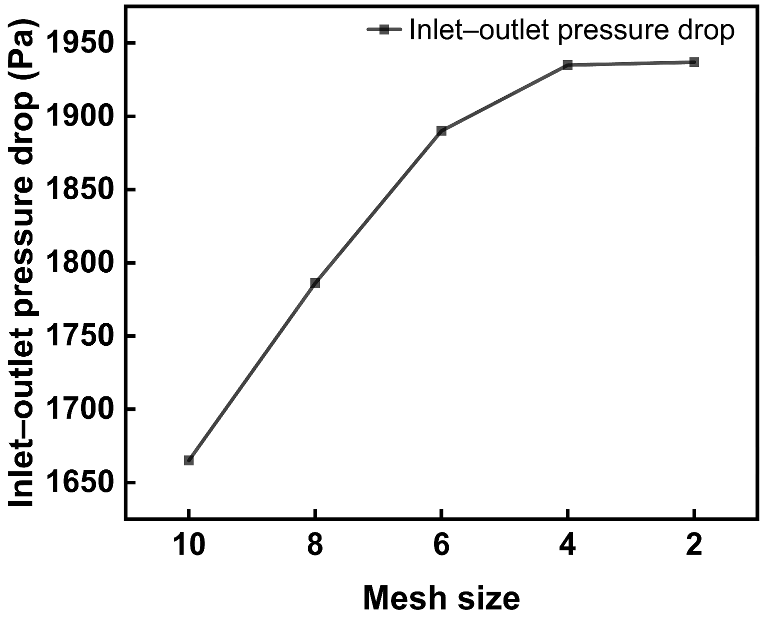
To verify the grid independence of the numerical results, comparative simulations were conducted using five different mesh densities under identical geometric configurations and inlet velocity conditions. The numbers of mesh elements considered were 4.28 × 10⁶, 4.44 × 10⁶, 5.26 × 10⁶, 8.48 × 10⁶, and 5.08 × 10⁷, respectively. The simulation results are presented in Figure 4, where the pressure loss across the parallel pipe bundle is used as the criterion for assessing grid independence.

The results indicate that when the number of mesh elements reaches approximately 8.48 × 10⁶, the inlet–outlet pressure loss becomes essentially stable, and further mesh refinement has a negligible influence on the numerical results. This confirms that grid independence was achieved. Considering both computational accuracy and computational cost, this mesh configuration was therefore adopted for all subsequent simulations.

2.5. Model Validation

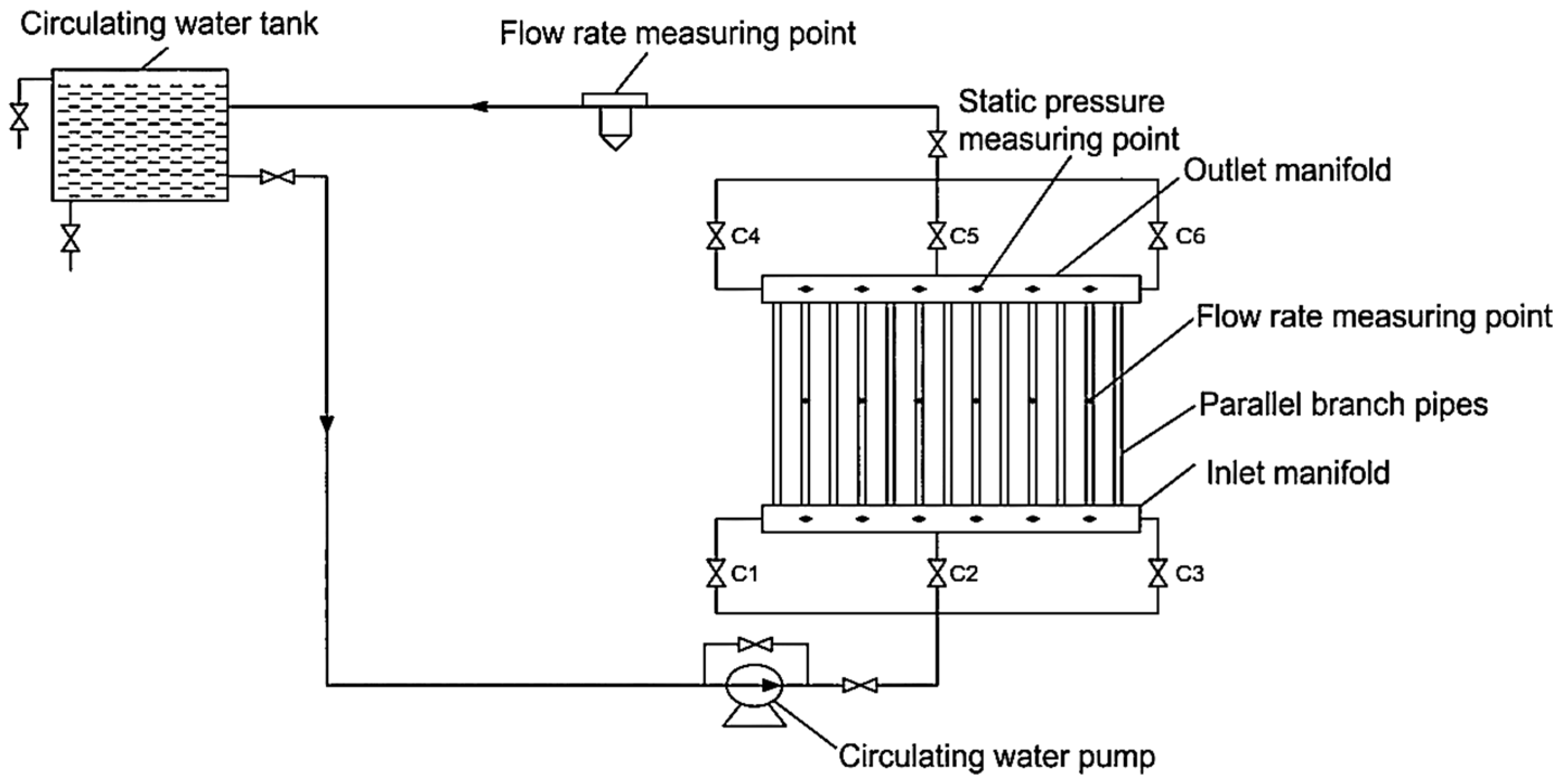
To verify the validity and applicability of the numerical model, experimental data for parallel pipe bundles reported in the literature were selected for comparison. Based on the flow distribution experiments conducted by Hu et al. [19] numerical simulations were performed for both co-flow and counter-flow configurations under identical geometric structures and operating conditions. The experimental apparatus had overall dimensions of 1.21 m × 0.39 m × 1.78 m, and its configuration is consistent with that of the numerical model, as illustrated in Figure 5.

Although the experimental data primarily provide static pressure measurements at the inlets and outlets of the branch pipes, the total pressure loss under steady incompressible flow conditions is dominated by static pressure differences. Therefore, agreement in static pressure distributions implies consistency in total pressure loss trends. In addition, the CFD-predicted total pressure loss was internally verified to exhibit the same relative variation patterns as the static pressure loss, further supporting the validity of the numerical model for pressure-loss analysis.

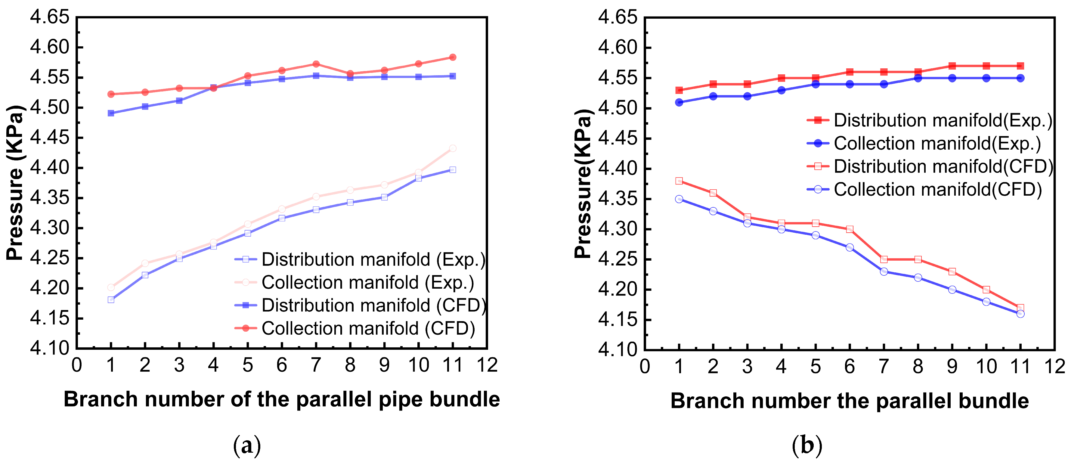
Under identical geometric configurations and boundary conditions, a comparative analysis of the static pressure distributions at the inlets and outlets of the parallel branch pipes was conducted. The results indicate that the relative errors between the numerical simulation results and the experimental measurements are all less than 10%, satisfying engineering accuracy requirements. This demonstrates that the established numerical model can reasonably capture the flow distribution and pressure loss characteristics within the parallel pipe bundle. Comparisons between the numerical and experimental static pressures at the inlets and outlets of each branch pipe are presented in Figure 6.

2.6. Limitations of Fluid Network Theory Under Vortex-Dominated Flow Conditions

Within the distribution manifold, collection manifold, and branch–manifold junction regions of a parallel pipe bundle, the real-world flows often exhibit pronounced three-dimensional characteristics, including flow separation, recirculation zone formation, and the coexistence of vortex structures across multiple scales. Induced by geometric discontinuities, changes in flow direction, and velocity gradients, these vortex structures locally enhance momentum exchange and energy dissipation. However, traditional one-dimensional fluid network models typically characterize energy losses solely through empirical resistance coefficients or frictional loss terms. Consequently, they fail to explicitly account for the effects of vortex-dominated three-dimensional flow.

Under vortex-dominated flow conditions, the simplifying assumptions inherent in conventional fluid network theory inevitably lead to a systematic underestimation of the actual pressure loss, as demonstrated by the numerical simulations and comparative analyses presented above. Consequently, reliance solely on traditional fluid network theory is insufficient to meet the accuracy requirements for predicting pressure losses in complex parallel pipe bundles operating at high Reynolds numbers.

In this context, it becomes essential to introduce a correction approach that quantitatively accounts for vortex-induced additional energy dissipation while preserving the original computational framework and engineering simplicity of fluid network theory. This requirement provides the theoretical foundation for the vortex-induced additional-loss correction model developed in the subsequent sections.

In the present study, the term “vortex-dominated flow” refers to flow regimes in which pressure loss is governed primarily by inertially induced three-dimensional vortical structures rather than by viscous friction alone. Practically, such regimes are characterized by high Reynolds numbers (Re > 10⁴), pronounced flow separation within manifolds and branch junctions, and significant deviations between one-dimensional fluid network predictions and CFD results, typically exceeding 15–20%. Under these conditions, vortex-induced energy dissipation becomes a dominant contributor to the total pressure loss.

3. Results and Discussion

3.1. Effect of Molten Salt Viscosity on Pressure Loss

To investigate the impact of viscosity, four distinct molten salt viscosities (0.0015, 0.003, 0.006, and 0.010 Pa·s) were examined at a fixed inlet velocity of 5 m·s⁻¹. Figure 7a,b present the pressure losses predicted by fluid network theory and those obtained from CFD simulations, respectively.

As illustrated in Figure 7, both fluid network theory predictions and CFD simulation results indicate that the pressure loss in each branch generally diminishes as molten salt viscosity increases and decreases along the flow direction. This behavior suggests that, at a fixed inlet velocity, viscosity modulates pressure loss primarily through its effect on the flow regime. An increase in viscosity reduces the Reynolds number, thereby weakening inertial effects. Consequently, velocity gradients and shear-layer intensity within the manifolds are reduced, suppressing flow separation and recirculation in the distribution manifold and branch–manifold junction regions and thereby reducing overall energy dissipation. However, for all viscosity conditions considered, pressure losses predicted by fluid network theory are consistently lower than those obtained from CFD simulations, indicating a systematic underestimation. Under low-viscosity conditions (μ = 0.0015 Pa·s), the relative deviation between the two approaches reaches a maximum of approximately 23% to 31%. As viscosity increases, this deviation gradually decreases.

Mechanistically, under conditions of low viscosity and high Reynolds numbers, inertial effects dominate flow behavior. In such regimes, large-scale vortex structures and recirculation zones are more likely to develop in the distribution manifold and branch–manifold junction regions. These three-dimensional vortical motions significantly enhance local momentum exchange and turbulent dissipation, thereby introducing additional energy losses. Because traditional fluid network theory is based on a one-dimensional, steady-flow assumption, its resistance models cannot explicitly account for vortex-induced dissipation, leading to a systematic underestimation of the actual pressure loss.

Comparisons between theoretical predictions and CFD results further reveal that pressure-loss distributions among individual branches in the real flow are more dispersed, reflecting flow non-uniformity within the manifolds and spatial variations in vortex intensity. As fluid viscosity increases at a fixed inlet velocity, the Reynolds number decreases and inertial instabilities are progressively suppressed. Consequently, shear-layer development and vortex intensity are weakened, resulting in reduced vortex-induced energy dissipation despite the concurrent increase in viscous resistance. This behavior provides direct physical justification for introducing a vortex-induced additional loss coefficient in the subsequent analysis.

3.2. Effect of Inlet Velocity on Pressure Loss

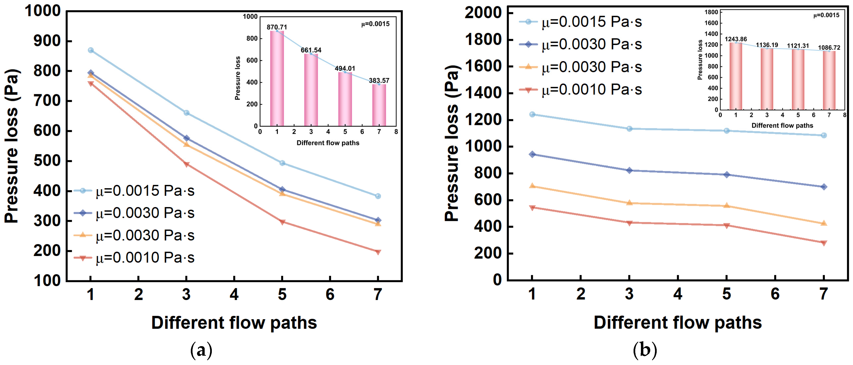
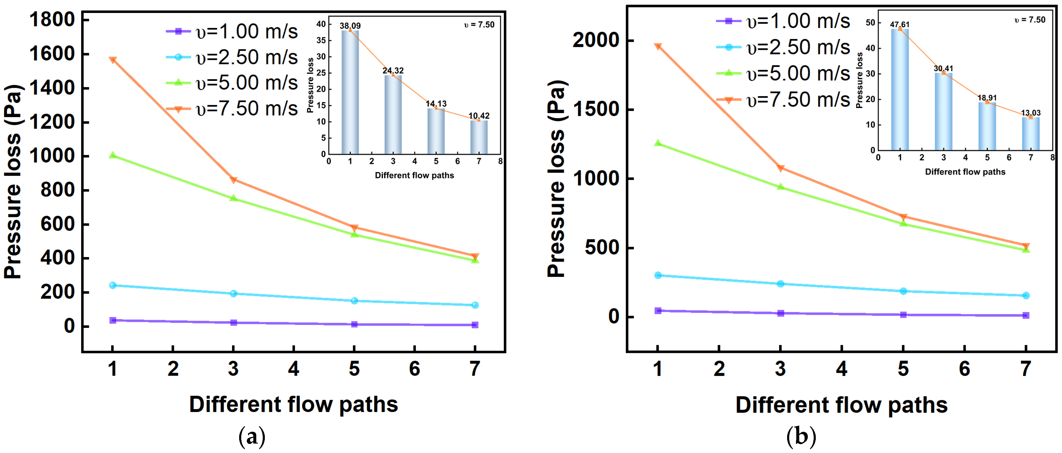
While maintaining constant structural parameters of the parallel pipe bundle and the physical properties of the molten salt held constant, four inlet velocities (1.0, 2.5, 5.0, and 7.5 m·s⁻¹) were selected to examine their effects on the pressure loss characteristics of individual branches. The corresponding pressure losses predicted by fluid network theory and obtained from CFD simulations are shown in Figure 8a and Figure 8b, respectively.

Results demonstrate a marked increase in pressure loss in each branch as the inlet velocity increases. This trend is consistently observed in both the fluid network theory predictions and the CFD simulation results. These findings identify inlet velocity as the dominant factor governing pressure loss in the parallel pipe bundle, primarily due to enhanced inertial effects at higher flow velocities. While theoretical calculations and CFD simulations exhibit similar trends, CFD results are consistently higher than the theoretical predictions under all inlet velocity conditions. Moreover, the deviation between the two approaches increases significantly with increasing inlet velocity. Under low-velocity conditions (1.0–2.5 m·s⁻¹), the discrepancy between theoretical predictions and CFD results is relatively small, whereas under high-velocity conditions (5.0–7.5 m·s⁻¹), it becomes much more pronounced. When the inlet velocity reaches 7.5 m·s⁻¹, the relative deviation increases to approximately 17–22%.

From a fluid dynamics standpoint, high-velocity conditions cause inertial forces to dominate, significantly intensifying interactions between the main flow and the distribution and collection manifolds, and intensifying the branch flows. This promotes flow separation within the manifolds, leading to the formation of large-scale recirculation zones and vortex structures. These three-dimensional vortex structures substantially augment local momentum exchange and turbulent dissipation, thereby inducing additional energy losses. In contrast, traditional fluid network theory is based on a one-dimensional steady-flow assumption, and its resistance models cannot explicitly account for the additional energy dissipation associated with such vortex-dominated flow structures. As a result, the underestimation of actual pressure loss becomes increasingly pronounced at higher inlet velocities.

3.3. Effect of Branch Diameter on Pressure Loss

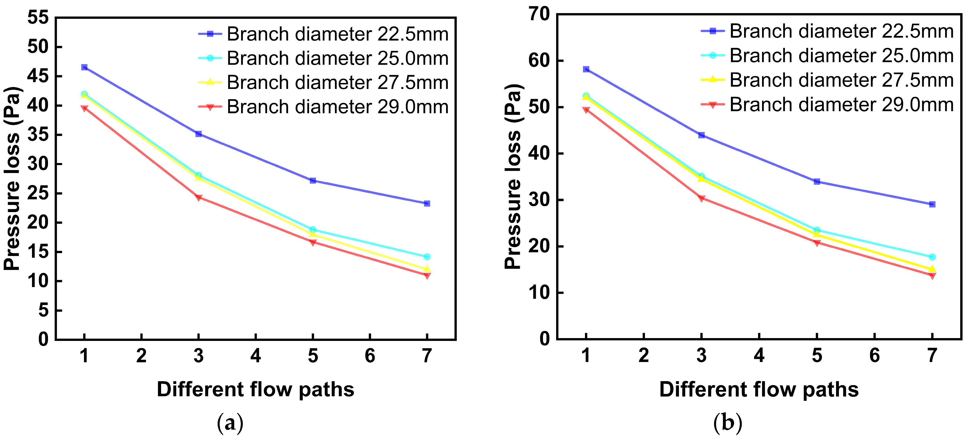
With the inlet velocity fixed at 5.0 m·s⁻¹ and the molten salt viscosity held constant, four branch diameters (22.5, 25.0, 27.5, and 29.0 mm) were selected to investigate their effects on the pressure loss characteristics of individual branches. The corresponding pressure losses predicted by fluid network theory and obtained from CFD simulations are shown in Figure 9a and Figure 9b, respectively.

As shown in Figure 9a,b, increasing the branch diameter from 22.5 to 29.0 mm results in a significant reduction in pressure loss for each branch in both the theoretical predictions and the CFD simulations. This trend aligns with fundamental principles of pipe flow. At a fixed inlet velocity, a larger branch diameter reduces the average flow velocity and frictional losses along the branch pipe, thereby mitigating local acceleration effects at the branch inlet and reducing overall pressure loss. However, across all branch-diameter conditions considered, CFD results remain significantly higher than those predicted by fluid network theory, with relative deviations consistently ranging from approximately 15% to 23%. This indicates that, although increasing the branch diameter effectively reduces the absolute pressure loss, it does not substantially mitigate the additional energy dissipation associated with three-dimensional vortex structures in the manifold–branch junction.

From a flow-mechanism perspective, increasing the branch diameter reduces flow velocity and frictional losses within the branch pipes. Nevertheless, flow splitting and merging processes within the manifolds are inevitably accompanied by flow separation, shear-layer development, and the formation of recirculation zones. These vortex structures, induced by geometric discontinuities and changes in flow direction, are clearly captured in the CFD simulations and continuously contribute to additional energy dissipation. In contrast, traditional fluid network theory primarily characterizes flow losses using one-dimensional frictional loss models and therefore cannot explicitly represent vortex-dominated three-dimensional dissipation mechanisms. As a result, a stable and systematic underestimation of the actual pressure loss is observed across different branch-diameter conditions. It is thus concluded that branch diameter primarily modulates the absolute magnitude of pressure loss. Conversely, its impact on the relative proportion of vortex-induced additional energy dissipation remains limited.

3.4. Effect of Manifold Cross-Sectional Ratio on Pressure Loss

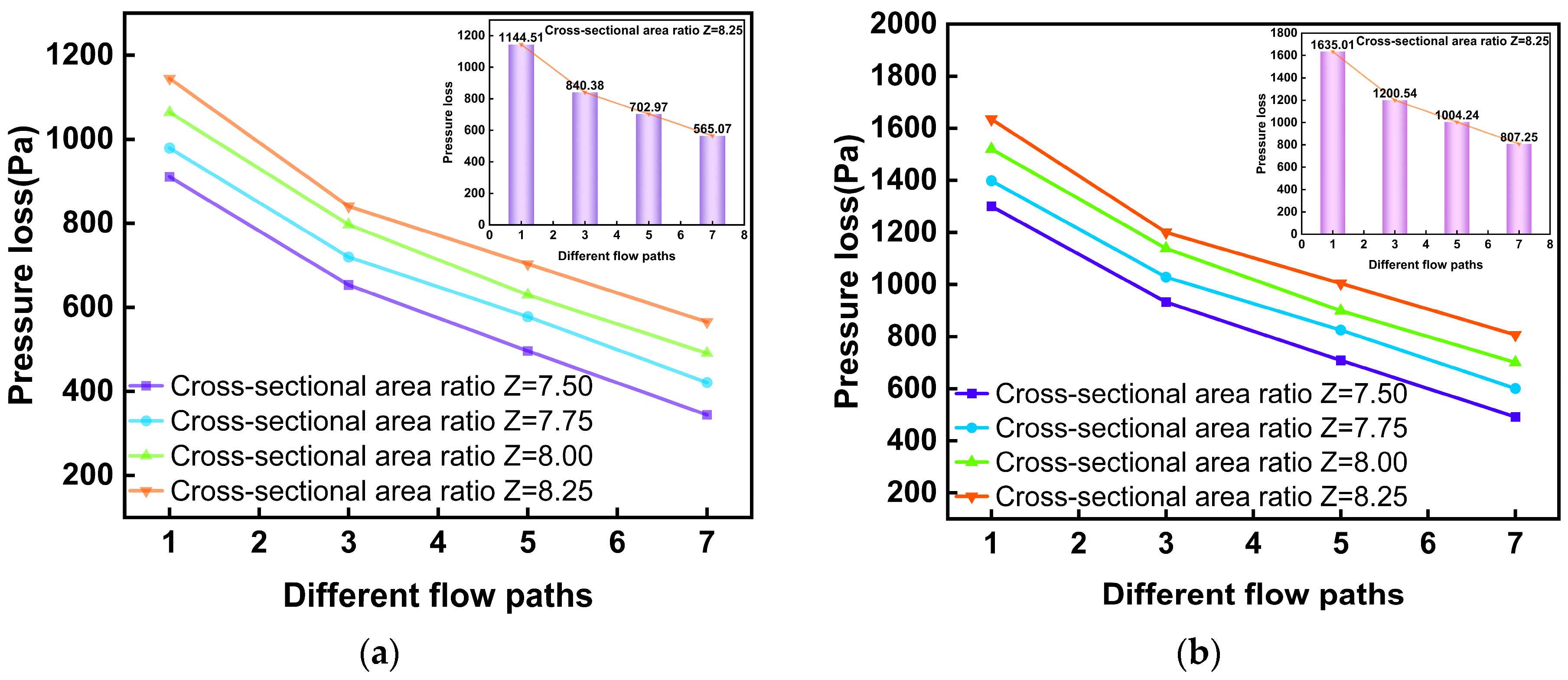
With the physical properties of the molten salt, inlet velocity, and other structural parameters held constant, four manifold cross-sectional ratios (Z = 7.50, 7.75, 8.00, and 8.25) were selected to investigate their effects on pressure loss in the parallel pipe bundle. The corresponding pressure losses predicted by fluid network theory and obtained from CFD simulations are shown in Figure 10a and Figure 10b, respectively.

Simulations indicate that the pressure loss in each branch of the parallel pipe bundle increases significantly with increasing manifold cross-sectional ratio Z. This trend is consistently observed in both fluid network theory predictions and CFD simulations, and for a given cross-sectional ratio, the pressure loss gradually accumulates along the flow direction. Notably, the deviation between fluid network theory predictions and CFD results also increases with increasing Z. When Z = 8.25, the relative deviation reaches approximately 25–33%, which is substantially higher than that observed under other operating conditions. This indicates that a larger manifold cross-sectional ratio amplifies the limitations of conventional fluid network theory in predicting pressure losses.

From a flow-mechanics perspective, increasing the manifold cross-sectional ratio reduces the mean axial velocity within the manifold, thereby alleviating flow acceleration near branch entrances and promoting a more uniform pressure distribution among branches. However, the enlarged manifold volume and extended flow paths also intensify three-dimensional flow development, including large-scale recirculation and vortex structures associated with flow splitting and merging. These vortex-dominated phenomena introduce additional energy dissipation that is not explicitly captured by one-dimensional network models, ultimately leading to increased prediction deviations despite the improvement in flow uniformity.

3.5. Effect of Manifold Arrangement on Pressure Loss

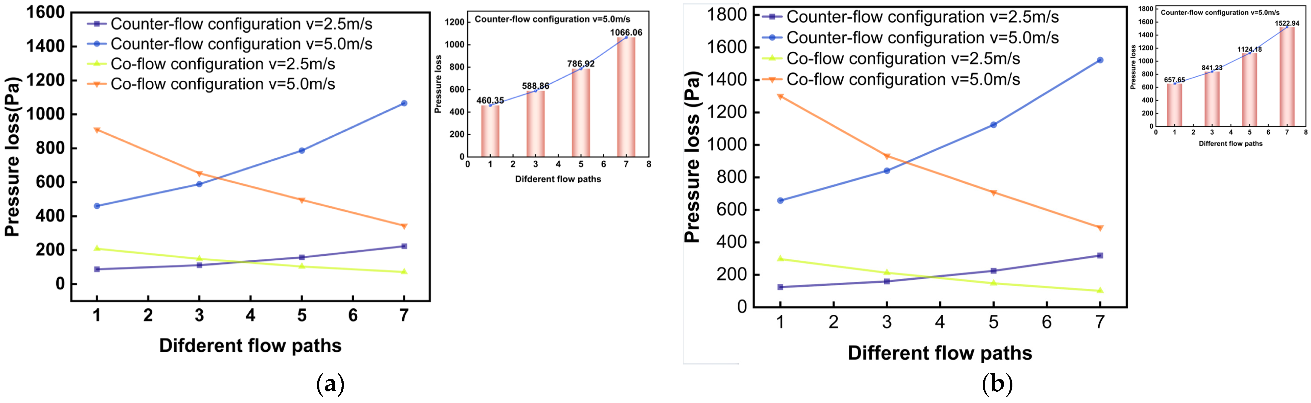
With the physical properties of the molten salt and the structural parameters of the parallel pipe bundle held constant, a comparative analysis was performed between co-flow and counter-flow manifold configurations. Inlet velocities of 2.5 and 5.0 m·s⁻¹ were considered. The corresponding pressure losses obtained from theoretical calculations and CFD simulations are presented in Figure 11a and Figure 11b, respectively.

Results reveal that, under identical inlet velocities, the pressure loss in the counter-flow arrangement substantially exceeds that in the co-flow arrangement. In the co-flow configuration, the pressure loss in each branch gradually increases with increasing flow path length, whereas in the counter-flow configuration, the maximum pressure loss is concentrated near the inlet region and decreases along the flow direction. Moreover, the deviation between fluid network theory predictions and CFD results is significantly larger for the counter-flow arrangement than for the co-flow arrangement. When the inlet velocity is 5.0 m·s⁻¹, the relative deviation under counter-flow conditions reaches approximately 27–36%, demonstrating that manifold arrangement plays a pivotal role in determining both pressure-loss characteristics and prediction accuracy.

From a flow-mechanics perspective, the counter-flow configuration induces opposing momentum directions between the inlet and outlet manifolds, which intensify velocity gradients and shear layers. This promotes stronger flow separation, recirculation, and vortex interaction, resulting in substantially higher energy dissipation compared with the co-flow arrangement.

Taken together, the preceding analyses indicate that molten salt viscosity, inlet velocity, branch diameter, manifold cross-sectional ratio, and manifold arrangement all exert significant influences on the pressure-loss behavior of the parallel pipe bundle. Conditions of low viscosity, high inlet velocity, large manifold cross-sectional ratios, and counter-flow arrangements are prone to generating strong three-dimensional vortex structures, thereby leading to additional energy dissipation. Under all investigated operating conditions, conventional fluid network theory consistently underestimates the actual pressure loss, and the prediction deviation increases markedly with increasing vortex intensity. These numerical findings clearly demonstrate the need to modify traditional fluid network theory to account for additional energy losses induced by vortex-dominated flows.

4. Correction Using a Vortex-Induced Additional Loss Coefficient

To quantitatively account for the additional pressure loss induced by vortices, a correction coefficient $\alpha$ is introduced into the conventional fluid network theory model. This section first analyzes the formation mechanism of vortices in the pipe bundle, then details the fitting process of $\alpha$, and finally validates the corrected model.

4.1. Formation Mechanism of Vortex Regions in the Parallel Pipe Bundle

Physically, the vortex-induced correction coefficient $\alpha$ represents the cumulative energy dissipation associated with three-dimensional vortex structures that are not explicitly resolved in conventional one-dimensional fluid network theory. In complex manifold–branch systems, abrupt changes in flow direction, strong velocity gradients, and geometric discontinuities give rise to large-scale recirculation zones and coherent vortical motions. These vortices enhance momentum exchange and drive the turbulent energy cascade, transferring kinetic energy from the mean flow to progressively smaller eddies, where it is ultimately dissipated by viscous effects.

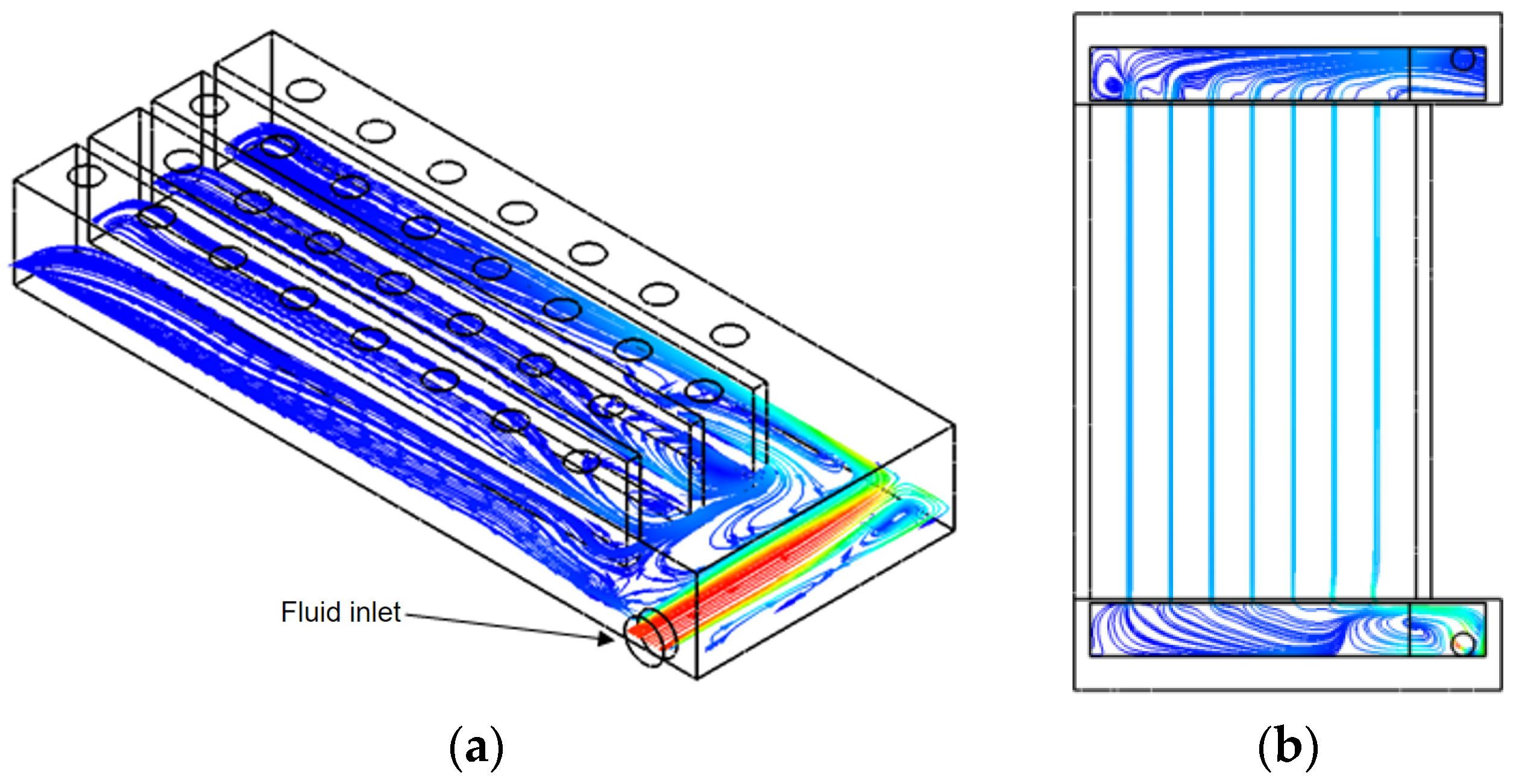
Upon entering the distribution manifold of the parallel pipe bundle, the molten-salt flow typically exhibits turbulent behavior. Numerical simulations reveal the widespread presence of vortex structures with pronounced rotational characteristics within the manifolds and branch–manifold junction regions, as illustrated in Figure 12. These turbulent eddies span a wide range of spatial scales and arise primarily from flow separation and geometric discontinuities. In the present study, the vortex-induced additional loss coefficient α is therefore interpreted as an equivalent global parameter that quantifies the integrated contribution of multi-scale vortex structures to overall energy dissipation, with dominant contributions originating from large-scale vortices generated in the manifold and branch–junction regions.

From a fluid mechanics perspective, turbulence involves the generation, evolution, and breakdown of vortices across a broad spectrum of spatial scales. Large-scale vortices, primarily governed by inertial forces, possess characteristic length scales comparable to the geometric dimensions of the flow field in the parallel pipe bundle. These vortices typically manifest as low-frequency, strongly rotating motions. Conversely, small-scale vortices are dominated by viscous forces, possess characteristic length scales much smaller than the pipe dimensions, and dissipate kinetic energy into thermal energy through viscous dissipation. During vortex evolution, energy is continuously transferred from large-scale to progressively smaller-scale vortices, constituting the classical turbulent energy cascade. Meanwhile, geometric discontinuities within the manifolds, velocity gradients, and changes in flow direction continuously trigger the generation of new vortex structures.

In parallel pipe bundles employed in heat exchangers, flow separation and recirculation are inevitable within the distribution and collection manifolds as well as at branch inlets, resulting in a highly non-uniform spatial distribution of vortex structures. These vortices not only significantly influence the flow distribution of molten salt among individual branches but also introduce additional energy dissipation, thereby increasing the actual pressure loss. Traditional fluid network theory, typically predicated on the assumption of one-dimensional steady flow, is well-suited for simplified geometries. However, it fails to explicitly account for additional pressure losses induced by three-dimensional vortex structures, which constitutes a primary reason for its limited predictive accuracy in complex flow fields such as parallel pipe bundles.

4.2. Fitting and Determination of the Vortex-Induced Additional Loss Coefficient

Traditional fluid network theory accounts for energy loss primarily through frictional resistance and empirical local loss coefficients, implicitly assuming quasi-one-dimensional flow. Under vortex-dominated conditions, however, additional energy dissipation arises from three-dimensional flow phenomena such as vortex stretching, vortex–vortex interaction, and flow separation, which cannot be explicitly represented by standard resistance formulations. The vortex-induced correction coefficient α is therefore introduced as an equivalent global parameter that incorporates the cumulative effect of vortex-induced dissipation along the flow path, effectively bridging the gap between three-dimensional flow physics and one-dimensional network modeling.

In the present study, the value of $\alpha$ is determined by comparing pressure-loss predictions from conventional fluid network theory with corresponding CFD simulation results. Rather than being treated as a local loss coefficient associated with a specific junction or component, $\alpha$ is defined as a global correction factor representing the integrated contribution of vortex-induced energy dissipation throughout the parallel pipe bundle.

To obtain an objective and robust estimate of the correction coefficient, the least-squares method—widely used in engineering data processing and error analysis—is employed. By minimizing the sum of squared residuals between theoretical predictions and CFD results, the optimal value of $\alpha$ is determined. The mathematical formulation of the least-squares method adopted in this study is given in Equation (13) [20,21].

$$\left\{\begin{array}{c}{a}_{11}{x}_1+a_{12}{x}_1+\cdots +a_{1n}{x}_n-b_1=0\hfill \\ a_{21}{x}_1+a_{22}{x}_1+\cdots +a_{2n}{x}_n-b_2=0\hfill \\ \cdot \cdot \cdot \cdot \cdot \cdot \cdot \cdot \cdot \cdot \cdot \cdot \hfill \\ a_{m1}{x}_1+a_{m2}{x}_1+\cdots +a_{mn}{x}_n-b_m=0\hfill \end{array}\right.$$

(13)

For each set of operating conditions, the residual error can be calculated using Equation (14).

$$\left.\begin{array}{c}{v}_1=b_1-f_1(x_1,x_2,\cdots ,x_n)\hfill \\ v_2=b_2-f_2(x_1,x_2,\cdots ,x_n)\hfill \\ \cdots \hfill \\ v_m=b_n-f_n(x_1,x_2,\cdots ,x_n)\hfill \end{array}\right\}$$

(14)

Based on the calculation results obtained under the various operating conditions examined in Section 3—including molten salt viscosity, inlet velocity, branch diameter, manifold cross-sectional ratio, and manifold arrangement—pressure loss data from the inlet of the parallel pipe bundle to the top of a selected branch were extracted. The CFD simulation results were used as reference values, and the corresponding vortex-induced additional loss coefficient, $\alpha$, was determined accordingly. The fitting results indicate that, within the parameter ranges investigated in this study, the value of $\alpha$ is primarily distributed between 1.15 and 1.37.

$$P_{IN}-P_{OUT}=\Delta P_M+\Delta P_{TP}$$

(15)

This additive formulation is consistent with the corrected pressure-loss expression given in Equation (15), in which the vortex-induced contribution is incorporated as an additional loss term. Accordingly, the correction coefficient $\alpha$ is introduced into the calculation of the frictional pressure loss, which is governed by the friction factor for molten-salt flow in the pipe, as expressed in Equation (16).

$$\Delta p_f=f\cdot {\displaystyle \frac{L}{D}}\cdot {\displaystyle \frac{\rho u^2}{2}}$$

(16)

According to fluid network theory, the friction factor has different formulations under different flow regimes. When the flow is in the laminar regime, the friction factor is given by Equation (17).

$$f={\displaystyle \frac{64}{Re}}$$

(17)

When the flow enters the turbulent regime, the friction factor is calculated using Equation (18).

$$f={\displaystyle \frac{0.316}{{Re}^{1/4}}}$$

(18)

Incorporating the vortex-induced additional loss coefficient $\alpha$ into the aforementioned frictional pressure loss model yields the corrected formulations for frictional pressure loss in the laminar and turbulent regimes can be obtained, as given in Equations (19) and (20), respectively.

$$\Delta p_{f,l}=\alpha \cdot f_l\cdot {\displaystyle \frac{L}{D}}\cdot {\displaystyle \frac{\rho u^2}{2}}$$

(19)

$$\Delta p_{f,t}=\alpha \cdot f_t\cdot {\displaystyle \frac{L}{D}}\cdot {\displaystyle \frac{\rho u^2}{2}}$$

(20)

where $\alpha$ is the vortex-induced additional loss coefficient.

Through this correction method, traditional fluid network theory is extended to effectively account for additional pressure losses induced by three-dimensional vortex structures, while preserving its original computational framework and engineering simplicity. Analysis of the fitted results indicates that the vortex-induced correction coefficient $\alpha$ increases with increasing inlet velocity and manifold cross-sectional ratio, and decreases with increasing fluid viscosity. In addition, counter-flow arrangements consistently yield higher values of $\alpha$ than co-flow configurations. These trends demonstrate that $\alpha$ is closely associated with operating and geometric parameters that intensify inertial effects and promote vortex generation.

Although $\alpha$ is treated as a global correction coefficient in the present study, it should be emphasized that it is obtained through least-squares fitting of CFD results under a specific geometric configuration and a defined range of operating conditions. Therefore, $\alpha$ should not be regarded as a universal constant applicable to arbitrary pipe networks. Instead, its numerical range (1.15–1.37) is valid for the investigated manifold geometry, branch arrangement, and Reynolds number range considered in this work, and recalibration may be required for different configurations or flow regimes. Nevertheless, the systematic dependence of $\alpha$ on Reynolds number, fluid viscosity, manifold cross-sectional ratio, and flow arrangement provides a clear physical basis for the future development of parametric or correlation-based expressions, enabling extension of the proposed correction framework to a wider range of flow conditions and configurations.

4.3. Validation of the Vortex-Induced Additional Loss Coefficient

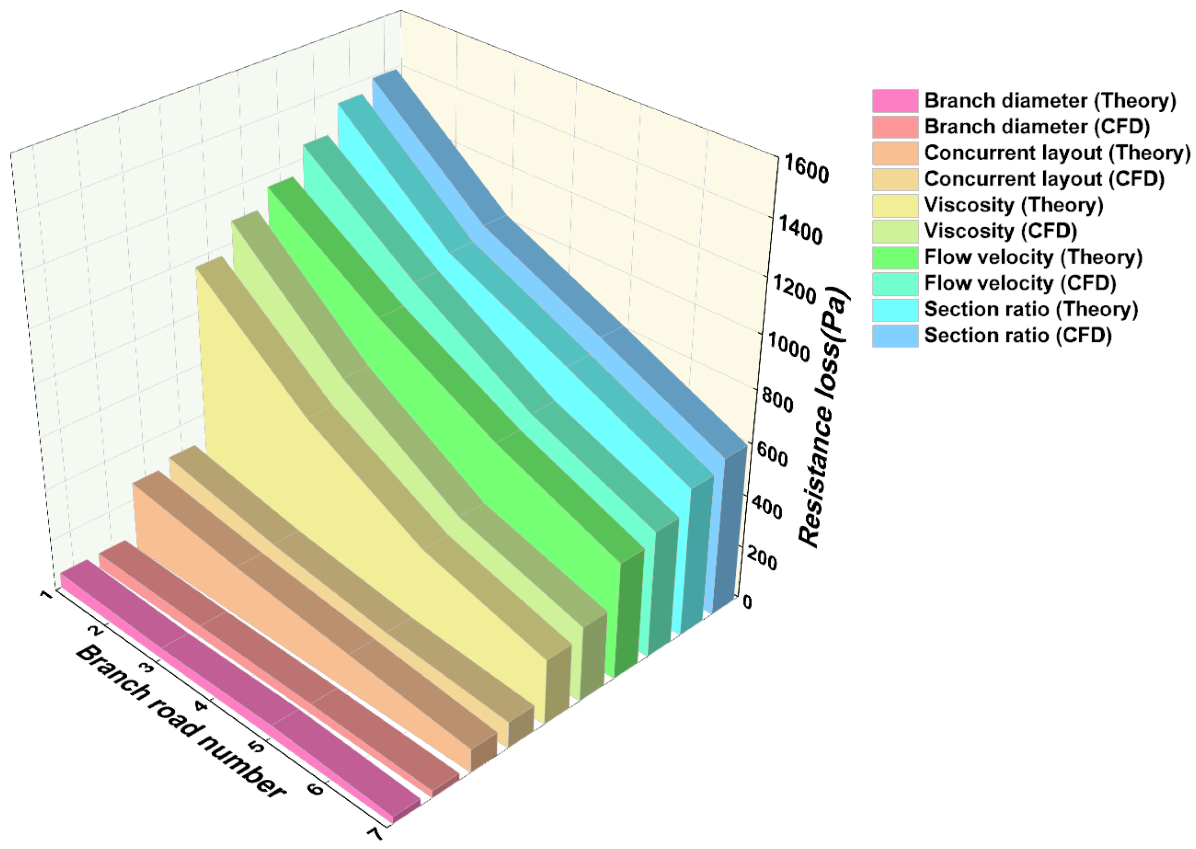
To validate the rationality and effectiveness of the proposed vortex-corrected model, representative operating conditions detailed in Section 3 were selected, including variations in molten salt viscosity, inlet velocity, branch diameter, manifold cross-sectional ratio, and manifold arrangement. For the co-flow configuration, the pressure loss from the inlet of the parallel pipe bundle to the top of the fourth-row branch was calculated, and the corrected theoretical predictions were compared with the corresponding CFD simulation results, as shown in Figure 13.

Comparative results demonstrate that, following the introduction of the coefficient α, corrected theoretical predictions exhibit strong agreement with numerical simulations in both trend and magnitude, with relative errors controlled within 5%, signifying a significant improvement in prediction accuracy compared with the uncorrected fluid network theory model. These results confirm the necessity and effectiveness of incorporating a vortex-induced additional loss coefficient into the pressure-loss model for parallel pipe bundles. The proposed correction method extends the applicability of fluid network theory under complex flow conditions, providing a more reliable theoretical framework for the engineering design and performance analysis of molten salt heat exchangers and related energy systems.

5. Conclusions

This study has addressed the limitations of traditional fluid network theory in accurately predicting pressure losses in complex parallel pipe bundles. Focusing on a molten-salt heat exchanger with a parallel pipe bundle, CFD simulations were integrated with theoretical analysis to systematically investigate pressure-loss mechanisms under vortex-dominated flow conditions. Based on these analyses, a vortex-based correction method for fluid network theory was proposed. The principal conclusions are summarized as follows:

(1)

Significant prediction errors are inherent to traditional fluid network theory under vortex-dominated conditions. The results demonstrate that conventional fluid network theory systematically underestimates pressure losses in complex parallel pipe bundles and manifold structures, particularly at high Reynolds numbers. Comparisons with CFD data indicate that prediction errors frequently exceed 20%, with deviations exacerbated under conditions of low fluid viscosity and high inlet velocity.

(2)

Vortex structures play a dominant role in intensifying pressure losses. Flow separation, recirculation zones, and inertial-dominated three-dimensional vortex structures were identified as the primary contributors to additional energy dissipation. These flow phenomena cannot be explicitly captured by conventional one-dimensional fluid network models, leading to a pronounced underestimation of the actual pressure loss.

(3)

Prediction accuracy is effectively enhanced through the introduction of a vortex-induced additional loss coefficient. The proposed vortex-induced correction coefficient $\alpha$ accounts for the excess energy dissipation associated with three-dimensional vortex structures. Based on least-squares fitting of CFD results, the value of $\alpha$ was determined to range from 1.15 to 1.37 within the investigated parameter space. Application of this correction reduces pressure-loss prediction errors to within 5% across various operating conditions, significantly improving the accuracy and engineering applicability of fluid network theory for complex flow systems. While effective within the flow regimes and parameter ranges considered, further validation is warranted to extend the proposed correction to other configurations.

References

1. Meißner, M.; Zimmer, D. Robust Modeling of Volumes for Dynamic Simulations of Thermo-Fluid Stream Networks. IFAC-PapersOnLine 2022, 55, 265–270. [Google Scholar] [CrossRef]
2. Saldana, M.; Gallegos, S.; Gálvez, E.; Castillo, J.; Salinas-Rodríguez, E.; Cerecedo-Sáenz, E.; Hernández-Ávila, J.; Navarra, A.; Toro, N. The Reynolds Number: A Journey from Its Origin to Modern Applications. Fluids 2024, 9, 299. [Google Scholar] [CrossRef]
3. Zhang, W.; Li, A.; Gao, R.; Yang, C.; Gao, X.; Du, F. Flow Performance Evaluation and Structural Optimization of the Dividing Manifold Systems Using Multi-Attribute Decision Analysis. J. Build. Eng. 2024, 85, 108652. [Google Scholar] [CrossRef]
4. Lin, L.; Duarte Batista, M.; Milesi Ferretti, N. State-of-the-Art Review on Measurement of Pressure Losses of Fluid Flow through Pipe Fittings. In NIST Technical Note 2206; National Institute of Standards and Technology: Gaithersburg, MD, USA, 2022. [Google Scholar]
5. Gao, G.; Wei, L.; Zhao, X.; Wan, M.; Li, H. The One-Dimensional Flow Pressure Loss Correction Model Based on the Particle Flow through Concrete Bend. Appl. Sci. 2024, 14, 8824. [Google Scholar] [CrossRef]
6. Li, D.; Liu, X.; Hou, P.; Liao, H.; Nie, R.; Jiao, Z. Experimental Investigation and Modeling of Local Resistance Coefficient of Reducing Pipe Using Selective Laser Melting. Alex. Eng. J. 2025, 117, 391–402. [Google Scholar] [CrossRef]
7. Smyk, E.; Stopel, M.; Szyca, M. Simulation of Flow and Pressure Loss in the Example of the Elbow. Water 2024, 16, 1875. [Google Scholar] [CrossRef]
8. Rosa, S.; Cavadas, A. Pressure-Loss Coefficients of Newtonian Fluid Flows in Axisymmetric Diffusers. Phys. Fluids 2025, 37, 103610. [Google Scholar] [CrossRef]
9. Mustafaoglu, M.; Yesilyurt, M.K.; Kotcioglu, İ.; Allahyari, M. Analysis of Flow Resistance in Trifurcation Fluid Networks. J. Appl. Fluid Mech. 2025, 18, 2550–2567. [Google Scholar] [CrossRef]
10. He, W.; Chen, Y.; Zhang, P.; Zhang, Q.; Ma, J. CFD-Based Prediction of Vortex-Induced Turbulent Flow in Urban Storm-Water Manholes: Insights into Gravity and Pressure Flow Dynamics. J. Water Process Eng. 2025, 77, 108346. [Google Scholar] [CrossRef]
11. Thorat, P.; Patil, R.; Patil, A.; Patil, S.; Padir, S.; Salunke, P. Flow Resistance Unveiled: Analyzing Major Losses in Pipeline Systems. Int. J. Mech. Eng. Technol. 2025, 16, 46–66. [Google Scholar] [CrossRef]
12. Zhang, J.; Wang, D.; Wang, W.; Zhu, Z. Numerical Investigation and Optimization of the Flow Characteristics of Bend Pipe with Different Bending Angles. Processes 2022, 10, 1510. [Google Scholar] [CrossRef]
13. Yao, L.; Liu, W.; Xu, K.; Yu, H.; Wu, J. Local Head Loss Range Analysis in Sudden-Expansion Pipelines Based on the S-A Turbulence Model. AQUA—Water Infrastruct. Ecosyst. Soc. 2026, 75, 1–16. [Google Scholar] [CrossRef]
14. Perumal, K.; Ganesan, R. CFD Modeling for the Estimation of Pressure Loss Coefficients of Pipe Fittings: An Undergraduate Project. Comput. Appl. Eng. Educ. 2016, 24, 180–185. [Google Scholar] [CrossRef]
15. Wu, Y.; Li, G.; Guo, P.; Zhang, H.; Ye, X.; Su, Y.; An, X. CFD Investigation on Resistance Balance of Complex Pipe Networks and Optimization Based on Artificial Neural Network. Ind. Eng. Chem. Res. 2024, 63, 22134–22149. [Google Scholar] [CrossRef]
16. Yazici, F.; Karadag, M.; Gokluberk, P.; KİBAR, A. Examining the Uniformity of Flow Distribution in Manifolds. J. Appl. Fluid Mech. 2024, 17, 998–1001. [Google Scholar] [CrossRef]
17. Li, B.; Park, T.S. Effects of Inlet and Outlet Layout on the Outflow Uniformity of Dividing Manifolds. J. Propuls. Energy 2025, 5, 33–47. [Google Scholar] [CrossRef]
18. Yaqub, M.W.; Chen, X. Interpretable Machine Learning for Three-Phase Flow Pressure Drop Prediction: A Comparative Study with CFD and Empirical Models. Chem. Eng. Sci. 2025, 310, 121542. [Google Scholar] [CrossRef]
19. Hu, X.; Yang, H.; Fan, F.; Yu, J. Experimental study on flow characteristics of parallel pipe groups with different arrangements. Chem. Equip. Pipelines 2021, 58, 24–29. (In Chinese) [Google Scholar]
20. Zou, L. Principle of least squares method and its simple applications. Sci. Technol. Inf. 2010, 282–283. (In Chinese). Available online: https://kns.cnki.net/kcms2/article/abstract?v=hGV7VzEtU5m0Q4QH5ukpTiabHAj-OCIOFWCRXETU8cbtMe6vZdjarQE_mpVLlna1FFuGLD6A5ttHwJFPsEVXqVffghl7teghQyv8hjBmOJAAmjrwpxjHBtkwMvZIGCjHEOrgB43lCQz4RVYo0dXw8jgwsldejRjpL59OeU7Svt_Pu0KpPalCLQMv2bOUAWZR&uniplatform=NZKPT&captchaId=d6ea69c9-7660-4538-a514-bcd77e1803fc (accessed on 18 December 2025).
21. Zhang, Q. Discussion on the principle of least squares method and its processing methods. Metrol. Test. Technol. 2020, 47, 75–76. (In Chinese) [Google Scholar] [CrossRef]
Figure 1. Structure of the parallel pipe bundle. (a) Physical model, (b) Finned tube channel, (c) Distribution manifold model, (d) Collection manifold model.
Fluids 11 00052 g001aFluids 11 00052 g001b
Figure 2. Schematic of flow in the distribution manifold. (a) first row, (b) second row.
Fluids 11 00052 g002
Figure 3. Schematic of flow in the collection manifold: (a) first row; (b) second row.
Fluids 11 00052 g003
Figure 4. Comparison of the inlet–outlet pressure drop of the parallel pipe bundle under different mesh sizes.
Fluids 11 00052 g004
Figure 5. Experimental setup for flow distribution in the parallel pipe bundle.
Fluids 11 00052 g005
Figure 6. Comparison of numerical and experimental static pressure distributions under different arrangement configurations. (a) Co-flow arrangement, (b) Counter-flow arrangement.
Fluids 11 00052 g006
Figure 7. Pressure loss under different viscosity conditions. (a) Fluid network theory predictions, (b) CFD simulation results.
Fluids 11 00052 g007
Figure 8. Pressure loss under different inlet velocity conditions. (a) Fluid network theory predictions, (b) CFD simulation results. The inset shows the variation in pressure loss across different flow paths under the highest velocity condition (7.50 m/s).
Fluids 11 00052 g008
Figure 9. Pressure loss under different branch diameter conditions. (a) Fluid network theory predictions, (b) CFD simulation results.
Fluids 11 00052 g009
Figure 10. Pressure loss under different cross-sectional ratio conditions. (a) Fluid network theory predictions, (b) CFD simulation results. The inset shows the variation in pressure loss across different flow paths at a cross-sectional area ratio (Z = 8.25).
Fluids 11 00052 g010
Figure 11. Pressure loss under different arrangement configurations. (a) Fluid network theory predictions, (b) CFD simulation results. The embedded image shows the variation in pressure loss under different flow paths in a counter-flow configuration (v = 5 m/s).
Fluids 11 00052 g011
Figure 12. Molten salt flow streamlines in the parallel pipe bundle. (a) First row, (b) Second row.
Fluids 11 00052 g012
Figure 13. Comparison of theoretical predictions and simulation results.
Fluids 11 00052 g013