Nonlinear Aerodynamic Load Response and Disaster Mechanism of Sedans in Strong Crosswinds

Abstract

To address the frequent disasters caused by strong crosswinds in Xinjiang’s “Hundred Miles Wind Zone,” this study utilizes a CFD numerical simulation method, validated by wind tunnel tests with an error of less than 5%, to systematically analyze the nonlinear response characteristics of a sedan’s aerodynamic loads under coupled conditions of vehicle speeds ranging from 60 to 100 km/h and crosswinds from 15.5 to 26.5 m/s. The results indicate that the sharp increase in leeward negative pressure, driven by flow separation, governs the escalation of aerodynamic loads. A distinct decoupling is observed between lateral force and drag: while lateral force scales linearly with vehicle speed, aerodynamic drag exhibits a nonlinear hysteresis. This is attributed to a “Flow Alignment Mechanism,” where the reduction in resultant yaw angle improves the leeward streamline topology, thereby mitigating drag growth. Furthermore, the rolling moment is identified as the dominant instability factor (peaking at 551.12 N·m). Conversely, the yawing moment saturates at high speeds due to an “Antagonistic Effect,” wherein dynamic pressure amplification is effectively counteracted by the shortening of the moment arm induced by the rearward migration of the Center of Pressure (CoP). These findings provide a robust theoretical basis for establishing speed limits and stability control strategies in extreme wind zones.

1. Introduction

With the progressive expansion of China’s highway network and the general rise in vehicle operating speeds, traffic safety issues induced by adverse environmental factors, such as strong crosswinds, are becoming increasingly severe. As a critical meteorological hazard, strong crosswind poses a direct threat to driving safety on expressways. When a vehicle travels at high speed, the intense lateral airflow can instantaneously generate immense aerodynamic lateral forces and yaw moments. This can easily cause the vehicle to deviate from its intended trajectory, experience sideslip, or even rollover, severely threatening the life and property of the occupants.

Numerous high-wind-prone areas exist in China, with the “Baili Wind Zone” [1] traversed by the G30 Lianyungang–Horgos Expressway being a prime example. This region is one of the most extreme wind zones along China’s highways, experiencing over 200 gale-force days annually and demonstrating adverse characteristics such as high wind intensity, prolonged duration, and stable direction. This persistent and severe extreme wind environment poses significant challenges to transportation safety on this highway section [2,3]. Statistical data indicate that the accident incidence induced by strong crosswinds on such wind-prone highway sections is significantly higher than on conventional road sections [4,5]. Therefore, conducting in-depth research on vehicle dynamic characteristics and their corresponding safe driving conditions in high-wind environments, specifically targeting the unique and harsh engineering background of the “Baili Wind Zone,” possesses both urgent practical significance and substantial theoretical value.

Over the past few decades, vehicle crosswind stability has evolved into a relatively mature field. In the early stages of research, scholars focused on theoretical modeling to define critical benchmarks for instability. For instance, Batista et al. [6] proposed static analysis models dedicated to determining the critical wind speed for vehicles under crosswind, establishing theoretical benchmarks for assessing typical instability modes such as rollover, sideslip, and rotation. William et al. [7] employed a 2-degree-of-freedom (2–DOF) vehicle lateral dynamics model to systematically analyze the vehicle’s lateral response under varying wind speeds and directions, constructing a theoretical framework for crosswind stability assessment applicable in the early design stages. Tiaming Huang et al. [8] utilized an evaluation framework built in CarSim to comprehensively consider the interaction of multiple factors, including vehicle speed, road grade, and crosswind angle. Qi Rui et al. [9] established an 8–DOF vehicle dynamics model considering crosswind effects. They used the phase-plane method to identify the vehicle’s state in the crosswind environment and designed a coordinated controller integrating Active Front Steering (AFS) and Direct Yaw moment Control (DYC) to maintain vehicle stability. Fu Limin et al. [10,11] adopted the yaw model method to compare the aerodynamic characteristics and wake vortex shapes of a sedan under multiple crosswind intensities.

The precision of theoretical models is highly dependent on the accuracy of aerodynamic load inputs, which are characterized using Computational Fluid Dynamics (CFD) simulations and wind tunnel tests to determine the vehicle’s aerodynamic properties. He Yongming et al. [12] developed static and dynamic models, utilizing automotive wind tunnel simulation software to calculate safe vehicle speed thresholds. Based on the simulation results, they calibrated the parameters of the dynamic model and established a safety evaluation model. Yuan Xiayi et al. [13] investigated the vehicle stability issues arising from trajectory deviation caused by sudden or sustained crosswinds during high-speed driving. They employed CFD simulations to calculate the vehicle’s aerodynamic characteristics under crosswind conditions and compared the results with wind tunnel test data. Yang Liechen et al. [14] simulated vehicle stability at various crosswind angles using CFD software 2022 R1 and subsequently validated the simulation results against wind tunnel experiments. The study demonstrated that the numerical error between simulation and experimental data was controlled within 5%, which not only confirmed the reliability of the CFD method but also established the significant role of numerical simulation as an effective supplement to wind tunnel testing. Zhang Kun [15] employed a stochastic gust model to simulate crosswinds, constructed a vehicle model using the dynamics simulation software CarSim, and conducted extensive simulation experiments and analyses of the vehicle operating in a crosswind environment. Chen Honglin [16] investigated the external flow field variations as two vehicles passed each other in a crosswind environment and analyzed the primary causes of the changes in vehicle aerodynamic characteristics during this process. Zhu et al. [17], through meticulous wind tunnel experiments, systematically explored the impacts of bridge deck effects and varying wind directions on aerodynamic coefficients. Ren Linlin [18] adopted the CFD method to study the transient characteristics of the vehicle’s flow field under various unsteady crosswind conditions, obtaining the vehicle’s aerodynamic coefficients and analyzing the flow field surrounding its body. Cooper and Watkins [19,20] investigated the influence of unsteady, turbulent crosswinds on vehicle aerodynamic performance and compared the differences among various turbulence characteristics. Yang et al. [21] utilized CFD and “mosaic” grid techniques to study how crosswinds near sand dunes affect a car’s aerodynamic loads and flow field. This study provides valuable insights for evaluating the effects of wind–sand on vehicle stability in desert areas. Cheli et al. [22] analyzed the aerodynamic effects on different vehicles under varying scenarios using a 1:10 scale model of heavy vehicles in a wind tunnel, simulating low, medium, and high turbulence. These studies provide a solid foundation for understanding aerodynamic loads.

As research progresses, the academic focus is shifting from idealized operating conditions to more complex, realistic environments. Brandt et al. [23] employed a coupled aerodynamic–vehicle dynamics numerical simulation approach to reveal the underlying mechanisms by which crosswinds affect stability under high-speed conditions. Recent studies have even begun to explore more extreme weather conditions. Zhang et al. [24] utilized numerical simulation to reveal the vehicle stability evolution mechanism under the combined effects of crosswind and ground sand. Guo et al. [25] used the CarSim platform to systematically analyze the impact of crosswinds on vehicle stability in a sand–dust environment. Focusing on the specific operating conditions of mountainous expressways, Wang Lu et al. [26] constructed a simulation environment in CarSim that included specific road and crosswind models. They innovatively adopted vehicle sideslip angle and lateral acceleration as driving risk evaluation metrics.

However, current research remains limited regarding the nonlinear coupling mechanisms of aerodynamic loads on high-speed vehicles within extreme wind environments, specifically winds exceeding Grade 10 in Xinjiang’s “Hundred Miles Wind Zone.” To address this gap, this study employs CFD numerical simulations grounded in the engineering context of the G30 Expressway, systematically investigating a matrix of operating conditions with vehicle speeds of 60, 80, and 100 km/h and crosswind velocities of 15.5, 19.0, 22.6, and 26.5 m/s. The primary objective is to unveil the topological evolution of the flow field under these combined scenarios. Specifically, this work elucidates the physical mechanisms governing the nonlinear hysteresis of aerodynamic drag and the saturation phenomenon of the yaw moment observed in the high-speed regime. Furthermore, the dominant aerodynamic factor precipitating vehicle instability is identified. These findings not only enrich the theoretical framework of ‘vehicle speed–wind speed’ coupling but also provide critical data support for establishing scientific speed limits and traffic control strategies in severe wind zones.

2. Numerical Simulation

2.1. Control Equations

In this study, the vehicle operates under strong crosswind conditions. The maximum vehicle speed is 100 km/h, and the maximum crosswind velocity is 26.5 m/s. The maximum Mach number in the flow field remains below 0.3. Consequently, the air is treated as a three-dimensional, incompressible Newtonian fluid. The simulation process involves no thermal exchange between the fluid and the vehicle body. Therefore, the energy equation is omitted. The simulation only satisfies the laws of conservation of mass and momentum. The equations are expressed as follows [16]:

(1)

Continuity equation

For an incompressible fluid, the density $\rho$ is constant. The continuity equation is simplified as follows:

$${\displaystyle \frac{\partial u}{\partial x}}+{\displaystyle \frac{\partial v}{\partial y}}+{\displaystyle \frac{\partial w}{\partial z}}=0$$

(1)

where $u$, $v$, and $w$ denote the velocity components in the $x$, $\mathit{y}$, and $z$ directions, respectively.

(2)

Momentum conservation equation

The fluid is a Newtonian fluid, and the dynamic viscosity $\mu$ is constant. The equations for the three directions ($x,y,z$) are expressed as follows:

$$\rho \left({\displaystyle \frac{\partial u}{\partial t}}+u{\displaystyle \frac{\partial u}{\partial x}}+v{\displaystyle \frac{\partial u}{\partial y}}+w{\displaystyle \frac{\partial u}{\partial z}}\right)=-{\displaystyle \frac{\partial p}{\partial x}}+\mu \left({\displaystyle \frac{{\partial }^{2}u}{\partial x^2}}+{\displaystyle \frac{{\partial }^{2}u}{\partial y^2}}+{\displaystyle \frac{{\partial }^{2}u}{\partial z^2}}\right)+f_x$$

(2)

$$\rho \left({\displaystyle \frac{\partial v}{\partial t}}+u{\displaystyle \frac{\partial v}{\partial x}}+v{\displaystyle \frac{\partial v}{\partial y}}+w{\displaystyle \frac{\partial v}{\partial z}}\right)=-{\displaystyle \frac{\partial p}{\partial y}}+\mu \left({\displaystyle \frac{{\partial }^{2}v}{\partial x^2}}+{\displaystyle \frac{{\partial }^{2}v}{\partial y^2}}+{\displaystyle \frac{{\partial }^{2}v}{\partial z^2}}\right)+f_y$$

(3)

$$\rho \left({\displaystyle \frac{\partial w}{\partial t}}+u{\displaystyle \frac{\partial w}{\partial x}}+v{\displaystyle \frac{\partial w}{\partial y}}+w{\displaystyle \frac{\partial w}{\partial z}}\right)=-{\displaystyle \frac{\partial p}{\partial z}}+\mu \left({\displaystyle \frac{{\partial }^{2}w}{\partial x^2}}+{\displaystyle \frac{{\partial }^{2}w}{\partial y^2}}+{\displaystyle \frac{{\partial }^{2}w}{\partial z^2}}\right)+f_z$$

(4)

where $\rho$ is the fluid density, $p$ is the pressure, $\mu$ is the dynamic viscosity coefficient, and $f$ is the body force. The term $\rho {\displaystyle \frac{\partial u}{\partial t}}$ represents the rate of velocity change with time in the $x$-direction. The convective term $\rho \left(u{\displaystyle \frac{\partial v}{\partial x}}+v{\displaystyle \frac{\partial v}{\partial y}}+w{\displaystyle \frac{\partial v}{\partial z}}\right)$ denotes the acceleration resulting from the non-uniform spatial velocity distribution. The term $-{\displaystyle \frac{\partial p}{\partial x}}$ indicates the pressure difference along the $x$-direction, which serves as the primary force driving fluid motion.

2.2. Geometric Models

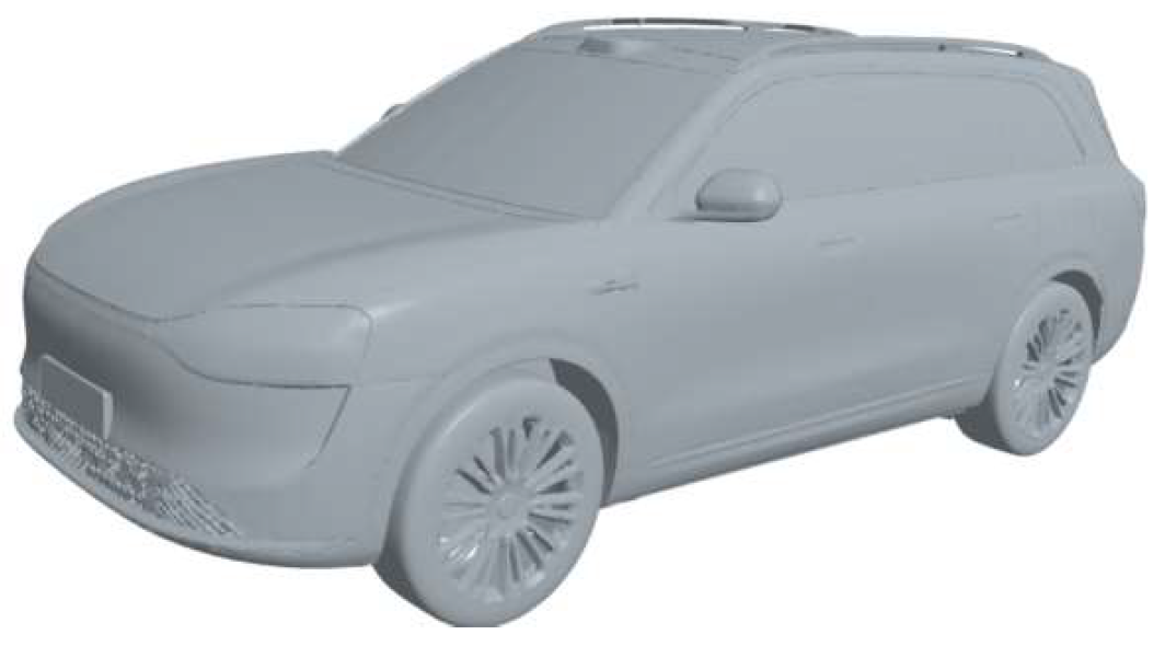
The subject of this study is a common highway passenger car. A three-dimensional geometric model was established using Solidworks 2024 software based on a sedan prototype. To enhance calculation efficiency and mesh quality while maintaining accuracy, the model was appropriately simplified. Key aerodynamic features, such as the body contour, were retained. Conversely, components with secondary impact on the lateral flow field were simplified. Specifically, the tire treads and complex chassis structures were omitted, and the wheels were treated as stationary relative to the vehicle body, while the ground effect was simulated using a moving wall boundary condition. The primary geometric and physical parameters of the established model are listed in

Table 1. Vehicle Model Parameters.

Parameter Name	Parameter Value
Length, L	4.57 m
Width, W	1.8 m
Height, H	1.68 m
Windward area, S	2.42 m2
Mass, m	1.5 t
Center of gravity height, hg	990 mm

.

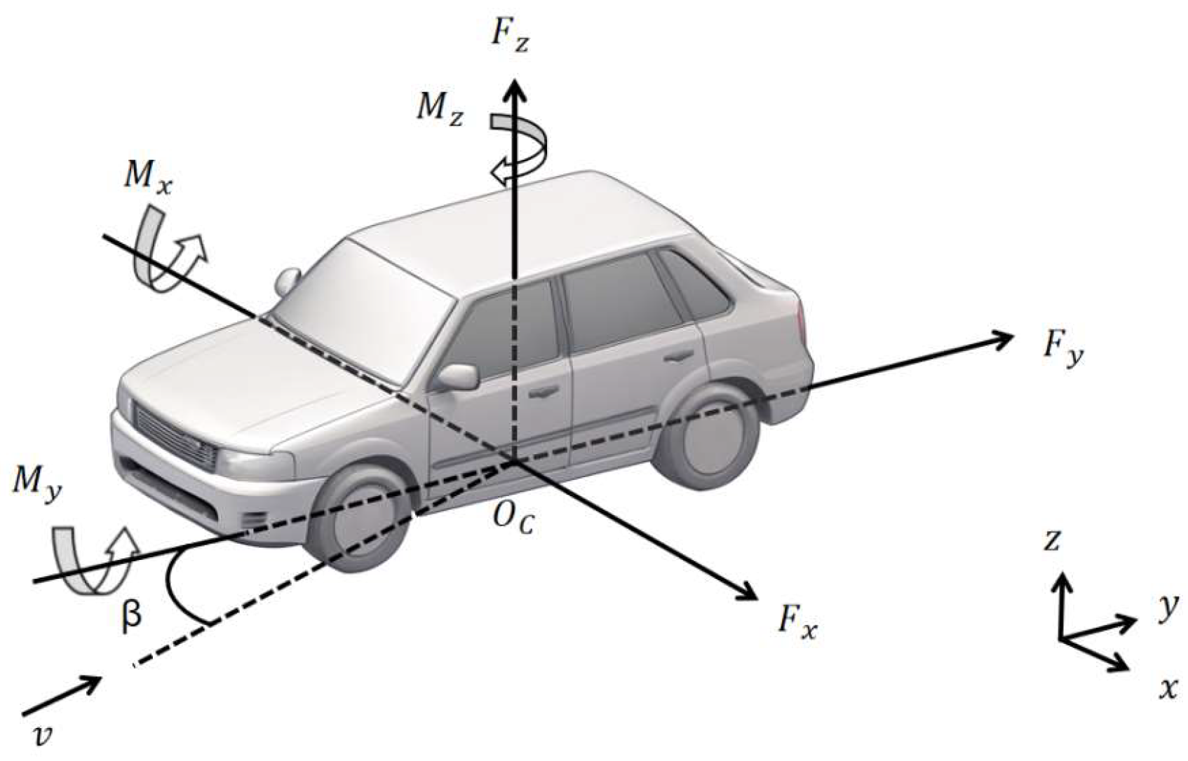
Taking the vehicle’s center of gravity (${\mathit{O}}_{\mathit{c}}$) as the origin of the aerodynamic coordinate system, the aerodynamic forces are resolved along the three axes. It is important to note that in this numerical model, the coordinate system is defined as follows: the y-axis aligns with the vehicle’s longitudinal driving direction (Drag force, ${\mathit{F}}_{\mathit{y}}$), the x-axis represents the lateral direction (Side force, ${\mathit{F}}_{\mathit{x}}$), and the z-axis represents the vertical direction (Lift force, ${\mathit{F}}_{\mathit{z}}$). Although this differs from the conventional body axis system where the x-axis typically denotes the forward direction, this setup is consistent throughout the simulation and analysis in this study. Here, ${\mathit{M}}_{\mathit{x}}$, ${\mathit{M}}_{\mathit{y}}$, and ${\mathit{M}}_{\mathit{z}}$ represent the aerodynamic pitching moment, rolling moment, and yawing moment, respectively, while β denotes the yaw angle, as shown in Figure 1.

In the complex high-speed driving environment, all six component aerodynamic forces acting on the vehicle contribute to varying degrees of disturbance to vehicle stability. This is particularly pronounced under crosswind conditions, where the magnitude of the aerodynamic forces (or their coefficients) is significantly greater than in no-crosswind scenarios, thereby posing a more severe threat to driving safety. The calculation formulas for the six-component aerodynamic forces are shown in

Table 2. Aerodynamic force and aerodynamic torque calculation formula.

Aerodynamic Force and Aerodynamic Torque	Calculation Formula
Aerodynamic lateral force $F_x$	${\mathit{F}}_{\mathit{x}}\mathit{=}\frac{\mathit{1}}{\mathit{2}}{\mathit{\rho }\mathit{\nu }}_{\mathit{\infty }}^{\mathit{2}}{\mathit{AC}}_{\mathit{S}}$
Aerodynamic drag $F_y$	${\mathit{F}}_{\mathit{y}}\mathit{=}\frac{\mathit{1}}{\mathit{2}}{\mathit{\rho }\mathit{\nu }}_{\mathit{\infty }}^{\mathit{2}}{\mathit{AC}}_{\mathit{D}}$
Aerodynamic lift $F_z$	${\mathit{F}}_{\mathit{z}}\mathit{=}\frac{\mathit{1}}{\mathit{2}}{\mathit{\rho }\mathit{\nu }}_{\mathit{\infty }}^{\mathit{2}}{\mathit{AC}}_{\mathit{L}}$
Aerodynamic pitching moment $M_x$	${\mathit{M}}_{\mathit{x}}\mathit{=}\frac{\mathit{1}}{\mathit{2}}{\mathit{\rho }\mathit{\nu }}_{\mathit{\infty }}^{\mathit{2}}{\mathit{AlC}}_{\mathit{PM}}$
Aerodynamic rolling moment $M_y$	${\mathit{M}}_{\mathit{y}}\mathit{=}\frac{\mathit{1}}{\mathit{2}}{\mathit{\rho }\mathit{\nu }}_{\mathit{\infty }}^{\mathit{2}}{\mathit{AlC}}_{\mathit{RM}}$
Aerodynamic yawing moment $M_z$	${\mathit{M}}_{\mathit{z}}\mathit{=}\frac{\mathit{1}}{\mathit{2}}{\mathit{\rho }\mathit{\nu }}_{\mathit{\infty }}^{\mathit{2}}{\mathit{AlC}}_{\mathit{YM}}$

. This indicates that after the vehicle’s frontal projected area is measured, the corresponding aerodynamic forces and moments can be calculated from the formulas once the force and moment coefficients are obtained through CFD simulation [27].

In the formula, A represents the projected frontal area of the vehicle, ρ is the air density, $v_{\infty }$ is the relative speed, $l$ is the wheelbase, and $C_S$, $C_D$, $C_L$, $C_{PM}$, $C_{RM}$, and $C_{YM}$ are the aerodynamic lateral force coefficient, drag coefficient, lift coefficient, aerodynamic trim moment coefficient, roll moment coefficient, and yaw moment coefficient, respectively.

2.3. Computational Domain and Meshing

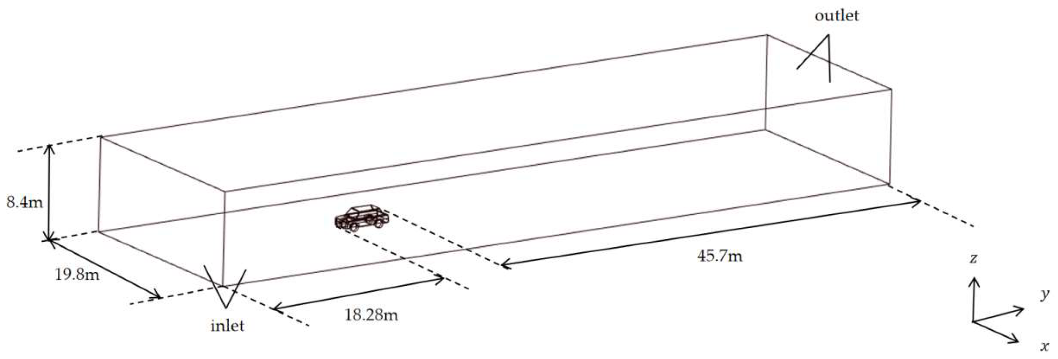
A rectangular computational domain was established to simulate the wind tunnel, as shown in Figure 2. The total length of the domain is 15L, the width is 11W, and the height is 5H, where L, W, and H represent the vehicle length, width, and height, respectively. The inlet boundary is located 4L upstream of the vehicle’s front, and the outlet boundary is 10L downstream of its rear. Both the windward and leeward lateral boundaries are positioned 5W from the vehicle.

Commonly used numerical simulation methods for steady-state crosswind include the yaw model method, the crosswind introduction method, and the synthetic velocity method. The synthetic velocity method, which defines the magnitude and direction of the velocity inlet, offers superior efficiency in mesh processing. Its numerical results demonstrate a consistent trend with experimental data and yield small errors [28]. Therefore, this paper adopts the synthetic velocity method. The boundary corresponding to the vehicle’s windward side is designated as the velocity inlet, while the leeward boundary is set as the pressure outlet, as shown in Figure 2. The resultant wind velocity ${\nu }_{res}$ and the effective yaw angle $\beta$ are calculated as follows [29]:

$${\nu }_{res}=\sqrt{{{\nu }_d}^2+{{\nu }_{\omega }}^2}$$

(5)

$$\beta =arctan\left({\displaystyle \frac{{\nu }_{\omega }}{{\nu }_d}}\right)$$

(6)

where ${\nu }_d$ is the driving speed of the vehicle; ${\nu }_{\omega }$ is the crosswind speed.

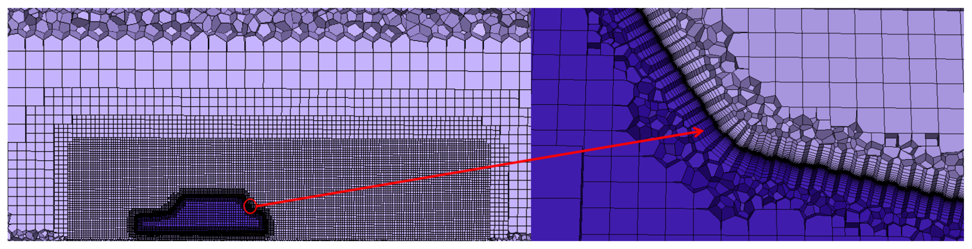
To ensure computational efficiency and simulation accuracy, the computational domain was discretized using unstructured grids via the ANSYS Fluent 2022 R1 Meshing module. Considering the vehicle’s complex curved surfaces and narrow gaps, as well as the large scale of the external flow field, the Mosaic-based Poly-Hexcore strategy was selected, as illustrated in Figure 3. This technology generates high-quality polyhedral grids near the vehicle body to precisely fit geometric boundaries while automatically filling the core region with orthogonal hexahedral grids, thereby effectively reducing the total grid count and enhancing solution convergence.

The specific mesh generation parameters are established as follows. First, during the surface mesh reconstruction stage, a combination of global size control and local refinement was adopted. The minimum and maximum surface mesh sizes were set to 0.02 m and 0.5 m, respectively, with a growth rate of 1.2. To accurately capture body edges and component gaps, curvature and proximity adaptive refinement functions were enabled. The curvature normal angle was set to 12°, and the number of cells per gap was set to 1, ensuring the resolution accuracy of the vehicle’s geometric features. Secondly, in the volume mesh generation stage, the global minimum mesh size remained 0.02 m, while the maximum size was relaxed to 0.64 m. A peel layer of 1 was set to achieve a smooth transition of the flow field mesh from the near-wall region to the far-field region. Finally, to accurately simulate viscous sublayer flow and boundary layer separation, prism layer meshes were generated on the vehicle surface. A smooth transition algorithm was employed, with the total number of boundary layers set to 15, an interlayer growth rate of 1.2, and a transition ratio of 0.272. To ensure the applicability of the Standard Wall Functions used in conjunction with the Realizable $\mathrm{k}$-epsilon turbulence model, the dimensionless wall distance $y^{+}$ was strictly monitored. Statistical analysis of the simulation results demonstrates that the $y^{+}$ values on the vehicle surface are predominantly distributed in the range of 32.5 to 285.6, with an average value of 68.2. This grid resolution ensures that the first mesh node is located within the logarithmic law region (30 < $y^{+}$ < 300), thereby guaranteeing accurate prediction of the boundary layer momentum transfer. Furthermore, it guarantees a smooth connection between the boundary layer mesh and the core mesh in the mainstream area, thereby avoiding numerical errors caused by abrupt changes in mesh size.

2.4. Verification of Grid Independence

Grid resolution is critical for the fidelity of numerical simulations. To verify the grid independence of the mesh employed in this study, a sensitivity analysis was conducted under a representative strong crosswind condition (vehicle speed: 80 km/h; crosswind velocity: 22.6 m/s).

Five grid configurations with varying densities were generated by systematically modulating the global maximum size and the minimum surface size. The specific settings for each scheme are detailed in

Table 3. Detailed mesh parameters for grid independence verification.

Grid Scheme	Global Max Size (m)	Surface Min Size (m)	Growth Rate	Total Elements
1	0.80	0.040	1.2	2,200,000
2	0.72	0.035	1.2	2,600,000
3	0.68	0.030	1.2	3,000,000
4	0.64	0.020	1.2	3,400,000
5	0.60	0.015	1.2	3,800,000

. As the grid density increased from Scheme 1 to Scheme 5, the global maximum size was reduced from 0.80 m to 0.60 m, and the minimum surface size was refined from 0.040 m to 0.015 m, resulting in a total element count ranging from approximately 2,200,000 to 3,800,000.

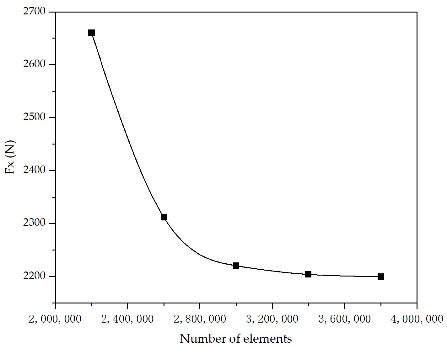
The aerodynamic lateral force ${\mathit{F}}_{\mathit{x}}$ was utilized as the convergence criterion. Figure 4 illustrates the variation in calculated ${\mathit{F}}_{\mathit{x}}$ with respect to the number of grid elements. As shown, the solution converges as the grid density increases. A significant variation in lateral force is observed as the element count rises from 2,200,000 to 3,000,000; however, the value stabilizes beyond 3,000,000 elements. The relative difference in ${\mathit{F}}_{\mathit{x}}$ between Scheme 4 (3,400,000 elements) and Scheme 5 (3,800,000 elements) is less than 0.2%.

Consequently, Scheme 4 (global maximum size: 0.64 m; minimum surface size: 0.02 m) was selected for all subsequent simulations. This configuration offers an optimal balance between computational accuracy and efficiency, ensuring that the mesh resolution is sufficient to capture the complex flow features around the vehicle.

2.5. Boundary Conditions and Turbulence Modeling

To accurately capture the vehicle’s aerodynamic characteristics in a complex wind environment and to minimize interference from the computational domain’s boundary layer effects, the boundary conditions for the computational domain were meticulously defined in this study. The specific settings are shown in

Table 4. Setting computational domain boundary conditions.

Name	Border Type
Inlet	$\mathrm{velocity}\mathrm{inlet},{\nu }_x$$=\mathrm{crosswind}\mathrm{speed},{\nu }_y$$=\mathrm{vehicle}\mathrm{speed},{\nu }_z$ = 0, turbulence intensity = 2.0%, turbulent viscosity ratio = 1.0
Outlet	pressure outlet, gauge pressure = 0, turbulence intensity = 2.0%, turbulent viscosity ratio = 1.0
Ground	$\mathrm{moving}\mathrm{wall},{\nu }_x$$=0,{\nu }_y$$=\mathrm{vehicle}\mathrm{speed},{\nu }_z$ = 0
Car body	no-slip wall
Walls	symmetry

.

Air density and viscosity were set to their default values, corresponding to the physical parameters of air at 25 °C. In the solver settings, this study adopted the pressure-based coupled algorithm to solve the pressure–velocity coupling equations. Compared to traditional segregated algorithms such as SIMPLE, the Coupled algorithm offers superior robustness and faster convergence for handling this type of steady-state external flow problem by simultaneously solving the momentum and pressure-correction equations. For spatial discretization, the Second-Order Upwind scheme was applied to all convective terms to ensure computational accuracy. This scheme, compared to the First-Order Upwind, significantly reduces numerical dissipation and more accurately captures the complex flow gradients around the vehicle body and in the wake region, which is a necessary guarantee for obtaining high-fidelity aerodynamic data. The Standard scheme was used for pressure interpolation. The Realizable $\mathrm{k}$-epsilon turbulence model was selected. The governing equations are as follows [30,31]:

$${\displaystyle \frac{\partial \left(\rho k\right)}{\partial t}}+{\displaystyle \frac{\partial \left(\rho k{u}_i\right)}{\partial x_i}}={\displaystyle \frac{\partial }{\partial x_j}}\left[\left(\mu +{\displaystyle \frac{{\mu }_t}{{\sigma }_k}}\right){\displaystyle \frac{\partial k}{\partial x_j}}\right]+G_k+G_b-\rho \epsilon -Y_M+S_k$$

(7)

$${\displaystyle \frac{\partial \left(\rho \epsilon \right)}{\partial t}}+{\displaystyle \frac{\partial \left(\rho \epsilon u_i\right)}{\partial x_i}}={\displaystyle \frac{\partial }{\partial x_j}}\left[\left(\mu +{\displaystyle \frac{{\mu }_t}{{\sigma }_{\epsilon }}}\right){\displaystyle \frac{\partial \epsilon }{\partial x_j}}\right]+C_{1\epsilon }{\displaystyle \frac{\epsilon }{k}}\left(G_k+C_{3\epsilon }{G}_b\right)-C_{2\epsilon }\rho {\displaystyle \frac{{\epsilon }^2}{k}}+S_{\epsilon }$$

(8)

where $\rho$ represents air density, $\mu$ represents turbulent viscosity, and $t$ represents time; $G_k$ represents the turbulent kinetic energy generation term due to the average velocity gradient; $G_b$ represents the turbulent kinetic energy generated by the action of buoyancy; $Y_M$ is the proportional factor of the pulsating expansion of the compressible turbulence dissipation rate. $C_{1\epsilon }$, $C_{2\epsilon }$ and $C_{3\epsilon }$ are empirical constants; ${\sigma }_k$ and ${\sigma }_{\epsilon }$ are the turbulent Prandtl numbers corresponding to the turbulent kinetic energy $k$ and the dissipation rate $\epsilon$, respectively; $S_k$ and $S_{\epsilon }$ are user-defined source terms, and the default values of CFD ${\sigma }_k$ = 1.0 and ${\sigma }_{\epsilon }$ = 1.3 are used.

2.6. Simulation Conditions and Validation of Numerical Results

To comprehensively investigate the aerodynamic characteristics of highway vehicles under various strong crosswind conditions, this study designed a series of simulation scenarios. The vehicle was set to travel at a constant velocity in a straight line at three typical highway operating speeds: 60 km/h (16.67 m/s), 80 km/h (22.22 m/s), and 100 km/h (27.78 m/s). The crosswind direction was uniformly set perpendicular to the vehicle’s direction of travel. Reflecting the actual meteorological characteristics of the “Baili Wind Zone,” this study selected four representative crosswind speeds: 15.5 m/s, 19 m/s, 22.6 m/s, and 26.5 m/s. These wind speeds cover a partial range from Level 7 (Gale) to Level 10 (Violent Storm), representing the severe wind environments that vehicles on expressways may encounter. By combining the three vehicle speeds with the four crosswind speeds, a total of 12 independent simulation scenarios were established. Their specific parameters are listed in

Table 5. Crosswind and vehicle speed combination scheme.

Operating Condition Number	Vehicle Speed (km/h)	Vehicle Speed (m/s)	Wind Speed (m/s)	Synthesis Speed (m/s)	Effective Yaw Angle $\mathit{\beta }$ (°)
1	60	16.67	15.5	22.77	43.0
2		16.67	19.0	25.26	48.7
3		16.67	22.6	28.08	53.6
4		16.67	26.5	31.06	57.8
5	80	22.22	15.5	27.1	34.9
6		22.22	19.0	29.24	40.5
7		22.22	22.6	31.7	45.5
8		22.22	26.5	34.58	50.0
9	100	27.78	15.5	31.68	29.2
10		27.78	19.0	33.65	34.3
11		27.78	22.6	36.00	38.9
12		27.78	26.5	38.56	43.8

.

To validate the accuracy and reliability of the CFD numerical simulation method, the simulation results were compared with wind tunnel test data published by Yuan Xiayi et al. [13], which were obtained at the Tongji University Ground Vehicle Wind Tunnel Center using a crosswind generator and equipped with a sextant floating frame strain balance, surface pressure measurement system, and PIV equipment. Focusing on conditions with yaw angles of 10° and 20° (velocity boundaries listed in

Table 6. Simulation Model Verification Conditions.

$\mathbf{Vehicle}\mathbf{Speed}{\nu }_{\mathit{x}}$ (km/h)	$\mathbf{Crosswind}\mathbf{Speed}{\nu }_{\mathit{y}}$ (km/h)	Effective Yaw Angle (°)	Synthesis Speed (km/h)
118	21	10	120
113	41	20	120

), CFD simulations were performed using a calibration model consistent with the wind tunnel test object, as illustrated in Figure 5. The comparative analysis revealed that the simulation error for both conditions was generally within 5% (

Table 7. Comparison of CFD Simulation and Experimental Results.

$\mathbf{Vehicle}\mathbf{Speed}{\nu }_{\mathit{x}}$ (km/h)	$\mathbf{Crosswind}\mathbf{Speed}{\nu }_{\mathit{y}}$ (km/h)	Project	${\mathit{F}}_{\mathit{x}}$/N	${\mathit{F}}_{\mathit{y}}$/N	${\mathit{F}}_{\mathit{z}}$/N	${\mathit{M}}_{\mathit{x}}$/(N·m)	${\mathit{M}}_{\mathit{y}}$/(N·m)	${\mathit{M}}_{\mathit{z}}$/(N·m)
118	21	Wind tunnel	735	731	517	−9	−561	−369
		Simulation	750	720	530	−9.4	−555	−365
		Error	2.0%	−1.5%	2.5%	−4.4%	1.1%	1.1%
113	41	Wind tunnel	1480	813	933	142	−1130	−670
		Simulation	1450	800	900	138	−1110	−690
		Error	−2.0%	−1.6%	−3.5%	−2.8%	−1.8%	3.0%

), demonstrating that the CFD method, meshing strategy, and boundary conditions employed in this study can accurately predict the vehicle’s aerodynamic characteristics under crosswind conditions, thereby ensuring high credibility for subsequent flow field analysis and vehicle dynamics research.

It should be noted that the wind tunnel validation was performed at a relatively high synthesis speed of approximately 120 km/h (Reynolds number ${\mathrm{R}}_{\mathrm{e}}$ ≈ 3.7 × ${10}^6$). While the current study covers a speed range of 60–100 km/h (${\mathrm{R}}_{\mathrm{e}}$ ≈ 1.8 × ${10}^6$–3.1 × ${10}^6$), the aerodynamic characteristics of bluff bodies like sedans are generally considered to be Reynolds-number-independent in the fully turbulent regime. However, we acknowledge that if the lower speed (60 km/h) falls near the critical Reynolds number for this specific geometry, the flow separation points might shift, potentially leading to slightly larger simulation errors compared to the validated high-speed condition. Since the critical speed for this vehicle geometry is not strictly defined in the available literature, the validation at 120 km/h serves as a reference for the mesh strategy’s capability to capture the dominant wake structures, with the understanding that prediction deviations may marginally increase at lower velocities.

3. Results and Discussion

This section analyzes the aerodynamic response mechanism of high-speed vehicles under strong crosswind conditions. The study is based on CFD numerical simulation results. It integrates flow field visualization contours and aerodynamic load data curves. The analysis focuses on three dimensions: flow field structure evolution, aerodynamic force response characteristics, and moment coupling characteristics.

3.1. Flow Field Characteristics Analysis

The alteration of the flow field structure is the fundamental cause of aerodynamic load generation. By analyzing the pressure and velocity field distributions under various combinations of vehicle speeds and crosswind velocities, the formation mechanism of aerodynamic asymmetry is revealed.

3.1.1. Pressure Distribution Characteristics and Pressure Difference Formation Mechanism

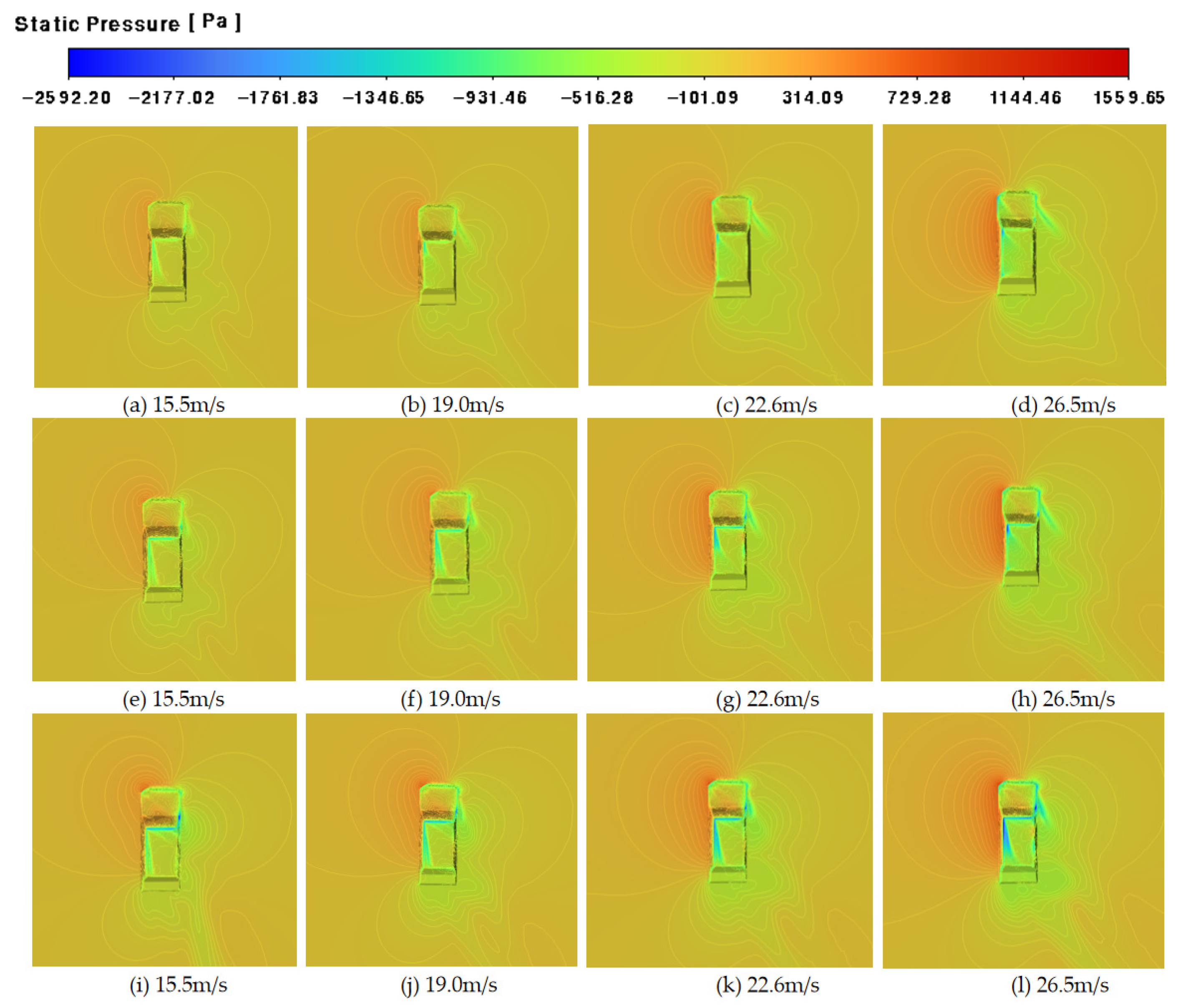
Figure 6 illustrates the static pressure distribution contours of the vehicle’s horizontal section under different conditions. As evident from the figure, the crosswind disrupts the flow field symmetry. This results in a significant pressure gradient on both sides of the vehicle body.

• Flow field asymmetry

As depicted in Figure 6, the left side (windward side) of the vehicle exhibits a distinct high-pressure zone. This corresponds to the stagnation positive pressure formed by airflow stagnation. Conversely, the right side (leeward side) and the rear exhibit low-pressure zones. This indicates that airflow separation occurred after passing the vehicle’s edges. This distribution characteristic of “windward high pressure” and “leeward low pressure” generates a significant pressure difference in the lateral direction.

2.

Dominance of Crosswind Velocity

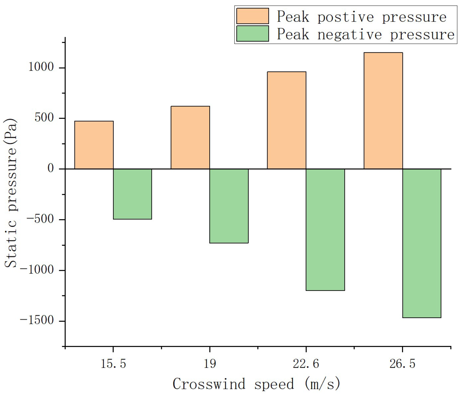
Figure 7 quantifies the variation in pressure extremes with crosswind velocity at a constant vehicle speed of 100 km/h. As the crosswind increases from 15.5 m/s to 26.5 m/s, the peak positive pressure on the windward side climbs from 474.47 Pa to 1150.09 Pa. The change in negative pressure on the leeward side is more drastic, dropping from −495.92 Pa to −1466.27 Pa. Quantitative analysis reveals that the leeward negative pressure is the primary contributor to the lateral pressure differential. This implies that large-scale vortex shedding and flow separation on the leeward side, rather than stagnation high pressure on the windward side, are the dominant mechanisms leading to the surge in aerodynamic lateral force.

3.

Dynamic Pressure Amplification via Vehicle Speed

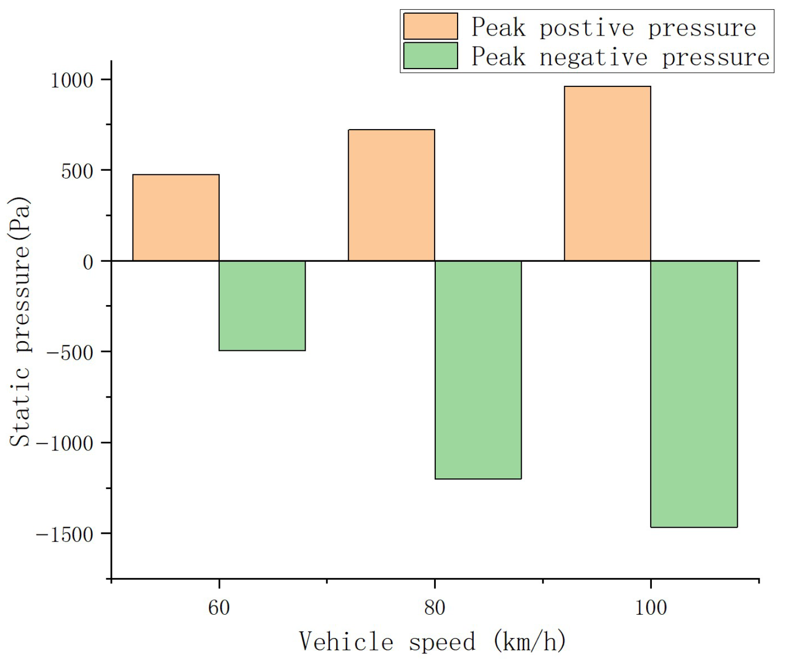
Figure 8 illustrates the influence of vehicle speed on pressure under a constant crosswind of 15.5 m/s. When the vehicle speed increases from 60 km/h to 100 km/h, the absolute values of both windward positive pressure and leeward negative pressure increase significantly. Specifically, the positive pressure rises from 479.55 Pa to 948.20 Pa. The negative pressure drops substantially from −509.92 Pa to −1458.86 Pa. This indicates that high-speed driving elevates the dynamic pressure level of the resultant airflow. Consequently, the pressure gradient on the vehicle body surface is amplified exponentially.

3.1.2. Topological Evolution of Velocity Field and Wake Structure Characteristics

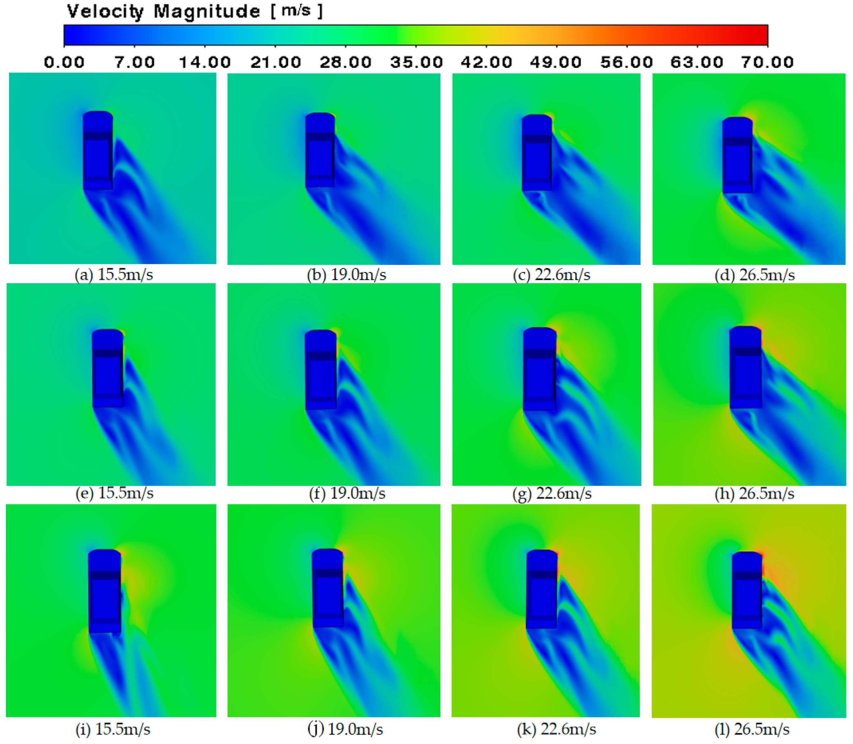
Figure 9 illustrates the velocity vector distribution on the horizontal section, visually revealing the evolutionary laws of the flow field under different operating conditions.

• Flow separation and wake deflection

As observed in Figure 9, on the leeward side (the right side of the vehicle), the airflow fails to attach to the vehicle body surface. Significant boundary layer separation occurs, forming a blue low-speed recirculation zone. As the crosswind velocity increases (from left to right, e.g., Figure 9a → Figure 9d), the resultant wind angle increases. This causes the wake region to deflect significantly toward the leeward side, while the width and extent of the low-speed wake region expand markedly.

2.

Shear effect of high-energy airflow

Under the coupled condition of a high vehicle speed of 100 km/h and a strong crosswind of 26.5 m/s (Figure 9l), the asymmetry of the flow field is most severe. Strong velocity gradients are formed at the windward corner of the vehicle front and the leeward corner of the vehicle rear (characterized by a sharp transition from dark blue to light green/yellow). This shear action exacerbates flow field instability and constitutes the fluid dynamic root cause inducing aerodynamic load fluctuations.

3.2. Analysis of Aerodynamic Forces and Moments

Based on the flow field visualization in Section 3.1, the evolution characteristics of aerodynamic loads are further investigated. This section aims to bridge the gap between microscopic flow topology and macroscopic load response. Through a comparative analysis of aerodynamic forces (Figure 10) and moments (Figure 11), the nonlinear response mechanism of the vehicle is revealed. Crucially, the variations in load curves are correlated directly with the specific evolution of velocity vectors and pressure distributions analyzed previously.

3.2.1. Linear Dominant Effect of Crosswind Velocity

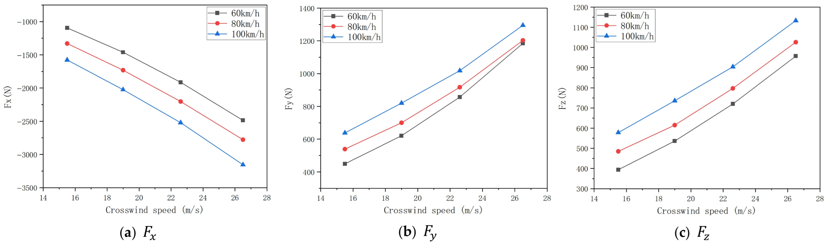
Figure 10 illustrates the variation in aerodynamic loads with crosswind intensity. Under constant vehicle speed, the lateral force $F_x$, drag force $F_y$, and lift force $F_z$ all exhibit a strictly monotonically increasing trend.

Taking the 80 km/h condition (Figure 10a) as a representative case, the absolute value of lateral force $F_x$ surges from 1329.78 N to 2777.09 N as crosswind speed increases from 15.5 m/s to 26.5 m/s. This high sensitivity is physically governed by the pressure field evolution shown in Figure 7. As the crosswind velocity rises, the negative pressure peak on the leeward side drops precipitously (from −495.92 Pa to −1466.27 Pa), creating a massive transverse pressure gradient. Simultaneously, the velocity vector field (Figure 9) confirms that the wake region deflects significantly towards the leeward side as the yaw angle $\beta$ increases. This expanding separation zone acts as the primary fluid dynamic driver forcing the linear surge of the lateral force.

3.2.2. Differentiated Load Response Under Vehicle Speed Coupling

Figure 10 reveals a complex coupling effect where aerodynamic drag and lateral force exhibit distinct response sensitivities to vehicle speed.

• Lateral Force Response ($F_x$): As illustrated in Figure 10a, under a strong wind of 26.5 m/s, the lateral force (black curve vs. blue curve) shows a sharp linear increase. This response is dominated by the dynamic pressure enhancement, which scales with the square of the resultant velocity ($F\propto {v^2}_{res}$). The flow field on the leeward side remains fully separated, offering no geometric mitigation.
• Drag Force Response ($F_y$): In contrast to the sharp rise in lateral force, the growth trend of aerodynamic drag $F_y$ in Figure 10b is markedly more moderate. This divergence is physically governed by a “Flow Alignment Mechanism,” as evidenced by the velocity vector fields in Figure 9. As detailed in Table 5, it is critical to note that under constant crosswind velocity, an increase in vehicle speed leads to a substantial reduction in the resultant yaw angle $\beta$ (e.g., decreasing from 57.8° to 43.8° under maximum crosswind). A comparative analysis of Figure 9d,l reveals that this reduction in $\beta$ effectively aligns the wake structure with the vehicle’s longitudinal axis. This topological evolution minimizes the projection area of the wake vortex in the drag direction and promotes flow reattachment on the leeward side. Consequently, this flow-induced streamline optimization generates a specific “drag-damping effect” that partially offsets the aerodynamic load amplification caused by rising dynamic pressure. As a result, the drag force demonstrates a nonlinear hysteresis characteristic, growing at a rate suppressed by the improving flow incidence, whereas the lateral force escalates without such geometric mitigation.

3.3. Aerodynamic Moment Coupling Characteristics

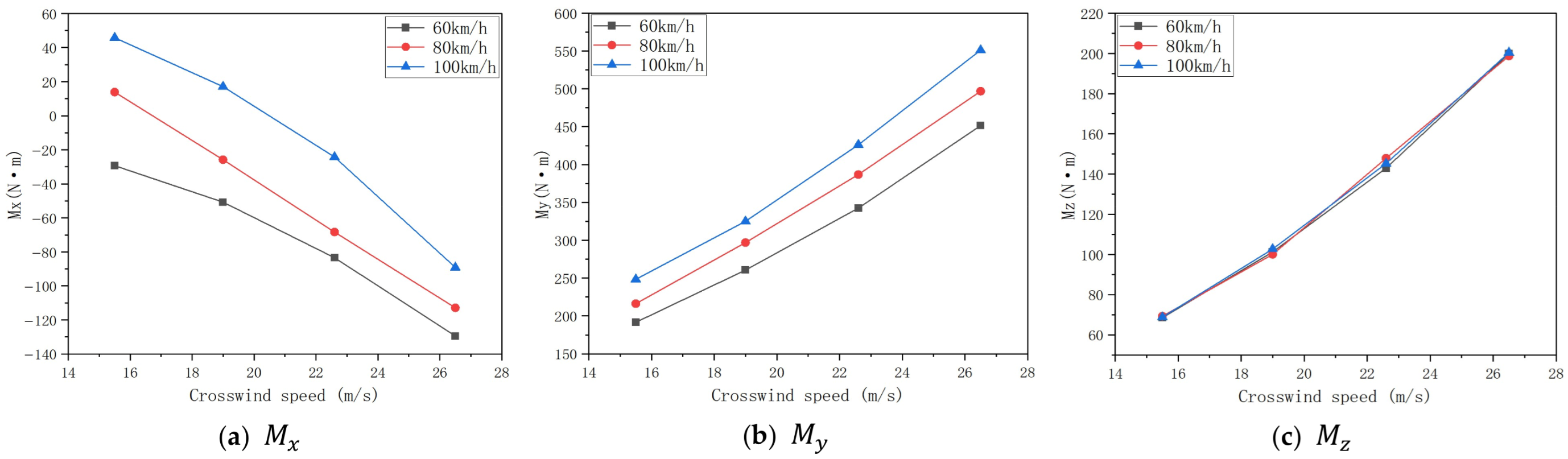
Aerodynamic moments directly determine the vehicle’s attitude stability. Based on the data in Figure 11, this section investigates the response mechanisms of pitching ($M_x$), rolling ($M_y$), and yawing ($M_z$) moments.

Prior to characterizing the primary hazard factors, a notable nonlinear feature is observed in the pitching moment ($M_x$). As illustrated in Figure 11a, $M_x$ exhibits a distinct sign reversal at specific critical wind speeds (e.g., the zero-crossing point at approximately 18 m/s under 100 km/h). This critical threshold signifies an aerodynamic equilibrium state, wherein the velocity-induced positive pitching moment (“nose-up”) is effectively neutralized by the crosswind-induced negative moment (“nose-down”). Despite this complex behavior, however, the magnitude of $M_x$ remains secondary compared to other moments in terms of destabilizing potential.

3.3.1. Identification of Crosswind Hazard Factors

In terms of absolute magnitude and stability threat, the rolling moment ($M_y$) clearly dominates the aerodynamic moment hierarchy. As shown in Figure 11, $M_y$ exhibits the highest sensitivity to crosswind velocity, significantly outstripping both the pitching and yawing moments. Taking the 100 km/h condition (Figure 11b) as a representative case, $M_y$ surges linearly from 248.40 N·m to a peak of 551.12 N·m. This consistent dominance confirms that in the extreme wind environment of the “Baili Wind Zone,” the primary aerodynamic risk is rollover instability driven by $M_y$, rather than the rotational deviation associated with $M_z$ or the pitch instability associated with $M_x$.

3.3.2. Mechanism of Yaw Moment Saturation: The Antagonistic Effect

A comparative analysis of Figure 10a,c reveals a critical nonlinear phenomenon. While the lateral force $F_x$ increases linearly with vehicle speed due to dynamic pressure amplification, the yawing moment $M_z$ exhibits a distinct “saturation state.” As shown in Figure 11c, the curves for 60 km/h, 80 km/h, and 100 km/h nearly overlap in the high-wind-speed region, maintaining a value of approximately 200 N·m. This indicates that $M_z$ stagnates and implies the existence of a self-limiting mechanism.

Detailed Analysis from the Flow Field Perspective: This study identifies the “Center of Pressure (CoP) Migration” as the physical root cause. The yawing moment is the product of the lateral force and its lever arm ($M_z=F_x·L_{arm}$). The saturation is the result of an antagonistic mechanism between the increasing force and the shortening lever arm:

• Force Component (Increasing): Higher vehicle speed increases dynamic pressure, linearly amplifying the lateral force $F_x$.
• Lever Arm Component (Decreasing): Simultaneously, the increase in vehicle speed reduces the effective yaw angle $\beta$. Analysis of the pressure contours in Figure 6 indicates that as $\beta$ decreases, the severe low-pressure separation zone on the leeward side shifts rearward. This topological change causes the aerodynamic center (CoP) to migrate towards the rear of the vehicle, moving closer to the center of gravity ($O_c$).

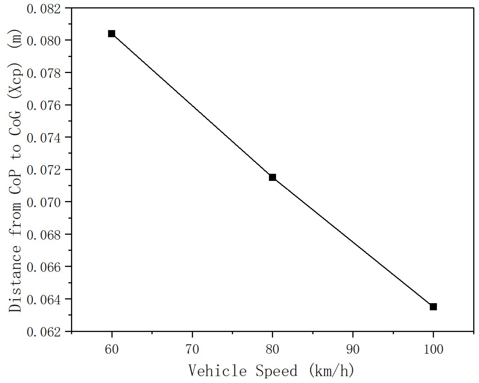
To quantify this mechanism, the effective aerodynamic lever arm ($X_{cp}=$|$M_z$/$F_x$|) was calculated for the strongest crosswind condition (26.5 m/s). As illustrated in Figure 12, the distance between the CoP and the Center of Gravity decreases strictly linearly with vehicle speed, dropping from 0.0804 m at 60 km/h to 0.0635 m at 100 km/h. This represents a significant 21% reduction in the moment arm.

The “force-increasing effect” of higher dynamic pressure is effectively neutralized by the “arm-shortening effect” induced by the flow field improvement. This proves that yaw instability possesses a self-limiting characteristic at high speeds, contrasting sharply with the continuously escalating rollover risk.

4. Conclusions

Focusing on the strong crosswind environment of the Xinjiang “Baili Wind Area,” this paper systematically investigates the aerodynamic characteristics of a passenger vehicle under combined operating conditions of different vehicle and wind speeds using CFD numerical simulation. Through flow field visualization and quantitative analysis of aerodynamic loads, the following conclusions are drawn:

• Leeward negative pressure is the dominant cause of aerodynamic loads. Strong crosswinds disrupt the symmetry of the flow field, inducing significant airflow separation and forming a low-pressure recirculation zone on the leeward side of the vehicle body. Research indicates that the absolute value of negative pressure on the leeward side generally exceeds the positive pressure on the windward side, and this pressure drops precipitously as wind speed increases. The dynamic pressure amplification effect induced by high vehicle speeds further exacerbates the lateral pressure gradient across the vehicle body. This constitutes the fundamental fluid dynamic mechanism responsible for the drastic increase in lateral force and rolling moment acting on the vehicle.
• Differentiated mechanisms for Drag and Lateral Force. Aerodynamic drag and lateral force exhibit distinct responses to vehicle speed coupling. While the lateral force grows linearly dominated by dynamic pressure, the aerodynamic drag $F_y$ shows a nonlinear hysteresis. This is attributed to the “Flow Alignment Mechanism” revealed by the velocity field analysis: the increase in vehicle speed reduces the resultant yaw angle $\beta$ (from 57.8° to 43.8°), which straightens the wake structure and mitigates flow separation. This topological improvement generates a drag reduction effect that competes with and partially offsets the dynamic pressure increase.
• Rolling moment is the primary hazard factor leading to vehicle instability. Among the various aerodynamic moments, the aerodynamic rolling moment $M_y$ exhibits the highest sensitivity to changes in crosswind velocity and possesses the largest magnitude. Taking the 100 km/h operating condition as an example, as the crosswind velocity increases, the amplitude of $M_y$ surges from 248.40 N·m to 551.12 N·m. This indicates that when driving in the Baili Wind Area, the paramount risk faced by vehicles is rollover accidents induced by the rolling moment, rather than simple rotation or sideslip.
• Mechanism of Yaw Moment Saturation (The Antagonistic Effect). In contrast to the monotonic surge observed in the rolling moment, the aerodynamic yawing moment ($M_z$) exhibits a saturation characteristic within the high-speed regime (stabilizing at approximately 200 N·m). This study identifies the “Center of Pressure (CoP) Migration” as the physical origin of this phenomenon, a mechanism quantitatively corroborated by the data in Figure 12. Specifically, the reduction in yaw angle at higher speeds drives the leeward low-pressure center rearward, resulting in a 21% reduction in the effective yaw moment arm (decreasing from 0.0804 m to 0.0635 m). Consequently, the linear amplification of lateral force is effectively neutralized by the shortening of the lever arm. This finding proves that yaw instability possesses an intrinsic self-limiting tendency at high speeds, distinguishing it from the escalating rollover risk.

In summary, for vehicles traversing strong crosswind regions like the “Baili Wind Zone,” the primary safety priority must be the mitigation of rollover risk induced by the rolling moment. Furthermore, the theoretical insights into yaw moment saturation (driven by CoP migration) and nonlinear drag hysteresis revealed in this study provide a rigorous aerodynamic basis for formulating graded speed limit strategies. Understanding that high-speed driving possesses an inherent self-stabilizing tendency regarding yaw motion allows for more scientifically optimized traffic regulations during extreme wind events.

References

1. Tang, H.; Zhou, Y.; Yang, J.; Pan, X. Analysis of mesoscale characteristics of strong wind in Baili Wind Zone of Xinjiang. Desert Oasis Meteorol. 2022, 16, 1–8. [Google Scholar]
2. Jiang, P.; Pan, X.; Xue, J.; Sha, Y. Comparative analysis of gale characteristics in the strongest wind region along Xinjiang railway. J. Meteorol. Environ. 2020, 36, 69–75. [Google Scholar]
3. Wang, X.; Liu, Y.; Lu, X.; Huang, A.; Du, F. Study on the characteristics of refined hourly wind speed in the Baili Wind Zone of Xinjiang from 2005 to 2020. Desert Oasis Meteorol. 2023, 17, 93–99. [Google Scholar]
4. Miao, Y.; Qin, R.; Yang, Y.; Zhang, Z. Continuity and characteristic analysis of gale data from representative stations in the Baili Wind Zone. Desert Oasis Meteorol. 2018, 12, 32–39. [Google Scholar]
5. Sun, S.; Zhang, G. Characteristics of vertical wind shear index in the surface layer of Baili Wind Zone in Xinjiang. Desert Oasis Meteorol. 2019, 13, 99–104. [Google Scholar]
6. Batista, M.; Perkovič, M. A simple static analysis of moving road vehicle under crosswind. J. Wind Eng. Ind. Aerodyn. 2014, 127, 105–113. [Google Scholar] [CrossRef]
7. William, Y.; Oraby, W.; Metwalley, S. Analysis of Vehicle Lateral Dynamics due to Variable Wind Gusts. SAE Int. J. Commer. Veh. 2014, 7, 485–494. [Google Scholar] [CrossRef]
8. Huang, T.; Feng, M.; Huang, J.; Ma, J.; Yi, D.; Ren, X.; Zhang, L.; Zeng, W. Aerodynamic stability of high-speed vehicle passing bridge tower in different lanes under crosswind conditions. J. Wind Eng. Ind. Aerodyn. 2023, 243, 105560. [Google Scholar] [CrossRef]
9. Qi, R.; Yang, J.; Zheng, Y.; Ni, Z.; Qi, S. Research on vehicle stability control under crosswind interference. J. Jiangsu Univ. Technol. 2024, 30, 52–62. [Google Scholar]
10. Fu, L.; Fu, Y. Numerical simulation study on crosswind effect of sedan external flow field with wheel rotation. J. Highw. Transp. Res. Dev. 2006, 23, 147–150. [Google Scholar]
11. Wang, F.; Fu, L. Numerical simulation study on the influence of crosswind on sedan aerodynamic characteristics. J. Harbin Inst. Technol. 2006, 38, 1255–1258. [Google Scholar]
12. He, Y.; Zhao, L.; Wang, F. Aerodynamic characteristics of ultra-high-speed vehicles under different crosswind conditions. J. Automot. Saf. Energy 2025, 16, 77–85. [Google Scholar]
13. Yuan, X.; Chen, L.; Li, S.; Wang, W. Simulation and evaluation of vehicle crosswind stability. Automot. Eng. 2019, 41, 1286–1293. [Google Scholar]
14. Yang, L.; Yuan, Z.; Qin, L.; Lv, H. Research on the influence of crosswind angle on vehicle stability. Autom. Appl. Technol. 2020, 2020, 206–208. [Google Scholar]
15. Zhang, K. Simulation Analysis and Countermeasure Research on the Impact of Crosswind on Highway Driving Safety. Ph.D. Thesis, Chang’an University, Xi’an, China, 2015. [Google Scholar]
16. Chen, H. CFD-Based Research on Aerodynamic Characteristics of Vehicles Passing Each Other in a Crosswind Environment. Master’s Thesis, Tianjin University of Science & Technology, Tianjin, China, 2023. [Google Scholar]
17. Zhu, L.D.; Li, L.; Xu, Y.L.; Zhu, Q. Wind tunnel investigations of aerodynamic coefficients of road vehicles on bridge deck. J. Fluids Struct. 2012, 30, 35–50. [Google Scholar] [CrossRef]
18. Ren, L. Study on Aerodynamic Characteristics of Heavy Commercial Vehicles under Several Typical Unsteady Crosswinds. Ph.D. Thesis, Jilin University, Changchun, China, 2015. [Google Scholar]
19. Cooper, K.R.; Watkins, S. The unsteady wind environment of road vehicles, part one: A review of the on-road turbulent wind environment. In Proceedings of the SAE 2007 World Congress & Exhibition, Detroit, MI, USA, 16–19 April 2007. [Google Scholar]
20. Watkins, S.; Cooper, K.R. The unsteady wind environment of road vehicles, part two: Effects on vehicle development and simulation of turbulence. In Proceedings of the SAE 2007 World Congress & Exhibition, Detroit, MI, USA, 16–19 April 2007. [Google Scholar]
21. Yang, W.; Wang, J.; Dong, Y. Effectiveness of three turbulence modeling approaches in a Crosswind–Sedan–Dune computational fluid dynamics Framework. Appl. Sci. 2024, 14, 7522. [Google Scholar] [CrossRef]
22. Cheli, F.; Ripamonti, F.; Sabbioni, E.; Tomasini, G. Wind tunnel tests on heavy road vehicles: Cross wind induced loads—Part 2. J. Wind Eng. Ind. Aerodyn. 2011, 99, 1011–1024. [Google Scholar] [CrossRef]
23. Brandt, A.; Jacobson, B.; Sebben, S. High speed driving stability of road vehicles under crosswinds: An aerodynamic and vehicle dynamic parametric sensitivity analysis. Veh. Syst. Dyn. 2022, 60, 3241–3265. [Google Scholar] [CrossRef]
24. Zhang, Z.; Chen, S.; Zhang, W. Numerical study on vehicle stability under crosswind conditions on desert highways. Sci. Rep. 2025, 15, 23552. [Google Scholar] [CrossRef]
25. Guo, B.; Gu, W.; Zhao, Z.; Zhang, X.; Igama, A. Simulation Research on Highway Driving Stability Early Warning System Under Crosswind Conditions. J. Adv. Transp. 2024, 2024, 8598011. [Google Scholar] [CrossRef]
26. Wang, L.; Xu, T.; Xue, H.; Lü, D. Simulation analysis of driving stability on mountainous expressway under crosswind. J. Transp. Inf. Saf. 2019, 37, 20–27. [Google Scholar]
27. Liu, J. Research on Driving Stability of Highway Curved and Sloped Sections in Crosswind Environment Based on Vehicle-Road Coupling. Master’s Thesis, Shijiazhuang Tiedao University, Shijiazhuang, China, 2020. [Google Scholar] [CrossRef]
28. Gong, X.; Gu, Z.; Li, Z.; Jiang, L.; Jia, X. Study on numerical simulation method of sedan aerodynamic characteristics under crosswind. Automot. Eng. 2010, 32, 13–16. [Google Scholar]
29. Zhang, M.; Zhang, J.; Long, J.; Li, Y.; Zou, Y.; Yin, D. CFD Numerical Simulation of Wind Field and Vehicle Aerodynamic Characteristics on Truss Bridge Deck under Crosswind. KSCE J. Civ. Eng. 2022, 26, 5146–5159. [Google Scholar] [CrossRef]
30. Hu, W. Research on Convective Wind Energy Harvesting Mechanism and Dust Recovery during Highway Vehicle Driving. Ph.D. Thesis, Hunan University, Changsha, China, 2022. [Google Scholar] [CrossRef]
31. Chen, Y.; Wang, Y.; Ma, R.; Hu, S. Study on aerodynamic characteristics and lateral stability of high-speed vehicles in wind-rain environment. Chin. J. Automot. Eng. 2025, 15, 59–68. [Google Scholar]
Figure 1. Aerodynamic force and aerodynamic torque on an automobile (Note: x-axis: Lateral; y-axis: Longitudinal; z-axis: Vertical).
Fluids 11 00049 g001
Figure 2. Schematic diagram of computational domain.
Fluids 11 00049 g002
Figure 3. The computational grid around the sedan (Left) and a detailed view of the boundary layer (Right).
Fluids 11 00049 g003
Figure 4. The aerodynamic lateral force F x changes with the number of grid elements.
Fluids 11 00049 g004
Figure 5. Validation model.
Fluids 11 00049 g005
Figure 6. Pressure distribution contours on the horizontal section under different wind speeds: (ad) vehicle speed of 60 km/h; (eh) vehicle speed of 80 km/h; (il) vehicle speed of 100 km/h.
Fluids 11 00049 g006
Figure 7. When the car speed is 100 km/h, the positive and negative pressure peaks vary with wind speed.
Fluids 11 00049 g007
Figure 8. When the crosswind speed is 15.5 m/s, the positive and negative pressure peaks vary with the vehicle speed.
Fluids 11 00049 g008
Figure 9. Velocity vector contours on the horizontal section under different wind speeds: (ad) vehicle speed of 60 km/h; (eh) vehicle speed of 80 km/h; (il) vehicle speed of 100 km/h.
Fluids 11 00049 g009
Figure 10. Variations of aerodynamic forces with crosswind speed at different vehicle speeds: (a) Aerodynamic lateral force Fx; (b) Aerodynamic drag Fy; (c) Aerodynamic lift Fz.
Fluids 11 00049 g010
Figure 11. Variations of aerodynamic moments with crosswind speed at different vehicle speeds: (a) Aerodynamic pitching moment Mx; (b) Aerodynamic rolling moment My; (c) Aerodynamic yawing moment Mz.
Fluids 11 00049 g011
Figure 12. Quantitative evolution of the aerodynamic lever arm ( X c p ) with vehicle speed under 26.5 m/s crosswind.
Fluids 11 00049 g012