Empirical Model for Predicting the Rheological Properties of Carbonated Slime Pulps

Abstract

The transport of carbonated slime pulps in pipelines is important for the acid lixiviation process that has developed in the nickel extraction industry in the eastern region of Cuba. This substance is a suspension of fine particles that behaves as a viscoplastic fluid. To address the lack of research conducted on carbonated slime pulps, we carried out an experimental investigation of the rheological properties of this substance over varied operational conditions. As the shear rates involved in the experiments covered more than two orders of magnitude, we fitted the flow curves to the Herschel–Bulkley model, which has been used in the past to model different suspensions. Through data analysis, we observed a transition in rheological behavior at a solid particle concentration of about 30%. Based on the trend of the flow curves, we built an empirical model to predict the rheological properties of slime pulps. In this model, the flow properties of the substance depend on the concentration of solid particles, the pH and the polydispersity index. Our empirical model exhibits high accuracy in predicting the flow properties of carbonated slime pulps. The results can be used to improve the efficiency of industrial processes involving these mineral suspensions.

1. Introduction

The transport of non-Newtonian fluids is important in different industrial processes, including food production, cosmetics manufacturing, and mining. The fluids involved in these processes contain fine particles that give them viscoplastic properties. A viscoplastic fluid is a substance that behaves as a solid when a small amount of shear stress is applied, but when the shear stress exceeds a certain threshold, the substance begins to flow. Two examples of these substances in everyday life are ketchup and toothpaste. A seminal study on viscoplastic fluids was conducted by Eugene Bingham, who investigated their flow in capillary tubes [1,2].

He found that, for certain substances, a pressure drop is required for their flow to begin. To model this kind of fluid, he proposed linear dependence between the shear rate $\dot{\gamma }$ and the shear $\tau$ [3]:

$$\begin{array}{c}\hfill \tau ={\tau }_0+{\mu }_p\dot{\gamma }\tau >{\tau }_0\\ \hfill \dot{\gamma }=0\tau \le {\tau }_0\end{array}$$

(1)

where ${\tau }_0$ is the yield stress and ${\mu }_p$ is the plastic viscosity. The simplicity of the Bingham model represents the basis of its use to model non-Newtonian fluids. For instance, the computation of ${\tau }_0$ and ${\mu }_p$ from experimental data requires only a linear regression. According to Litan et al. [4], the Bingham model effectively describes the rheological behavior of suspensions for shear rates in the range of 0 to 4 s⁻¹. However, according to Coussot, when the shear rate covers two or more orders of magnitude, the Bingham model no longer describes the fluid properties. Instead, viscoplastic fluids are often adjusted to the Herschel–Bulkley model [3,5], where there is a non-linear relationship between the shear rate and the shear stress:

$$\begin{array}{c}\hfill \tau ={\tau }_0+K{\dot{\gamma }}^n\tau >{\tau }_0\\ \hfill \dot{\gamma }=0\tau \le {\tau }_0\end{array}$$

(2)

This model contains three parameters: the yield stress ${\tau }_0$, the consistency index K, and the flow index n. For a shear-thinning fluid, $n<1$, whereas for a shear-thickening substance, $n>1$.

The existence of a yield point requires some discussion. According to previous studies [6,7], the value of yield stress depends on the method used to measure it. Some authors suggest the existence of two types of yield stress, dynamic and static, similar to the friction coefficient for solid bodies. According to Dinkgreve et al. [6], the dynamic yield point occurs when the shear stress decreases until the substance ceases to flow, while the static yield point is the critical shear stress at which the substance begins to flow as shear stress increases. It has been argued that for simple materials, both quantities must coincide [6].

The presence of a dispersed phase in a fluid gives it non-Newtonian properties. Examples of these substances are polymeric solutions, emulsions, and suspensions. For polymeric solutions, their rheological behavior depends on time because their motion causes the polymer chains to be rearranged or even broken [8]. In the past, researchers around the world devoted considerable effort to investigating the rheology of polymers [9,10,11,12,13] because of their importance in industry. Regarding emulsions, their flow properties depend on the fraction and size distribution of the dispersed phase. At a low content of the dispersed phase, the substance behaves as a Newtonian fluid, whereas at a high content, it acquires non-Newtonian properties, because the interaction between particles leads to their coalescence. In the food and pharmaceutical industries, oil emulsions are very important, and some investigations have focused on drop size distribution, the influence of viscosity on drop size, and the presence of solid particles [14,15,16,17,18,19]. Finally, suspensions are fluids that contain solid particles. Based on diameter size, the particles are classified as clay, silt, or sand. Clays are particles with a diameter of less than 3.9 $\mathsf{\mu }$m, silts are particles with a size between 3.9 and 62.5 $\mathsf{\mu }$m, and, finally, sand particles have a size between 62.5 $\mathsf{\mu }$m and 2 mm. Most studies on suspensions have been conducted on mixtures of clay and silt [20]. These kinds of particles give the substance viscoplastic properties. Some researchers have reported that millimetric particles also influence the substance’s rheological properties [4]. In the mining industry, some mineral suspensions have been investigated because of their importance in ore extraction; for example, studies have been conducted on the rheological properties of bentonite [21,22], goethita [23], and laterites from different deposits [23,24,25,26,27].

In this study, we investigate the properties of carbonated slime pulps, which are suspensions containing solid particles with diameters of less than 100 $\mathsf{\mu }$m. Their clay content is approximately 50%, their silt content is around 40%, and they contain a small percentage of fine sand. Previous investigations of carbonated slime pulps showed that the content of solid particles has a strong influence on their rheological properties. In brief, at concentrations of solid particles below 30%, the flow properties become nearly independent of the granulometric composition and the suspension behaves as a pseudoplastic fluid [27,28,29,30,31,32,33,34,35]. Nevertheless, for concentrations between 30% and 50%, the apparent viscosity (the ratio of shear stress to shear rate) increases due to the interactions among particles, and the substance acquires viscoplastic properties. Among the studies on the rheological behavior of carbonated slime pulps, we highlight a study by G.L. Perez [36]. In this study, the author conducts an experiment to measure the flow properties of this fluid at a solid particle concentration of 43% and a pH of 7.41. Unfortunately, experiments are not conducted at other concentrations or pH values. Moreover, the author does not take into account the polydispersity index, which influences the rheology of this substance.

The main goal of this research is to construct an empirical model capable of predicting the rheological properties of carbonated slime pulps. To this end, we conduct experiments measuring their flow curves under different conditions. Based on previous studies on suspensions and our experimental data, we use the concentration in weight of the solid particles (C), the pH, and the polydispersity index (s) as independent variables. The formulas of the model are designed to cover concentrations of solid particles between 17% and 50%, pH values in the range of 7.71 to 8.52, and polydispersity indexes in the range of 0.717 to 0.985. These intervals cover the operating conditions in the nickel industry. To our knowledge, no previous studies have been conducted that cover these ranges of operating conditions.

The transport of suspensions over long distances is a subject of growing importance due to its applications in industrial processes. These applications include mineral separation, hydraulic fracturing, food and pharmaceutical processes, and wastewater treatment. The transport of solid particles using a carrier fluid reduces energy consumption compared with other methods such as trucks or conveyor belts. Many investigations on the motion of suspensions and slurries have been carried out in recent decades. The aspects addressed are the particle sizes, the particle size distribution, the concentration of solid particles, settling and its relationship with mean velocity, the rheological properties of the fluid, and the pressure drop on different parts of a pipeline. Research on this topic is both experimental and numerical. In the field of experimental research, we highlight a study conducted by Turian and Yuan [37], who investigated the pressure drop in pipelines under four conditions: heterogeneous flow, homogeneous flow, moving bed flow, and stationary bed flow. The authors collected experimental data from the published literature and conducted experiments in a slurry pipeline. Their results are given in terms of the difference $f-f_w$, where f and $f_w$ are, respectively, the friction factors of the slurry and the water. Ultimately, they obtain the pressure gradient using the relation ${\displaystyle \frac{\Delta P}{\Delta L}}=2f{\displaystyle \frac{\rho V^2}{D}}$. In the study, Turian and Yuan discuss the importance of particle settling on the pressure drop and the dependence of settling on the flow mean velocity. More recently, Kaushal et al. [38] investigated the effect of the particle size on the pressure loss in a slurry flow in a horizontal pipeline. The volumetric flow Q was measured with an electromagnetic flow meter, whereas the pressure drop was measured with differential pressure transducers. The experiments were conducted in a 22 m long recirculating pipe. The sizes of solid particles were 125 $\mathsf{\mu }$m and 440 $\mathsf{\mu }$m. The flow velocity varied from 1 to 5 m/s. The authors found that the pressure drop increases with velocity for the slurry with solid particles of 125 $\mathsf{\mu }$m. However, for particles of 440 $\mathsf{\mu }$m, the pressure drop increases for velocities around V = 5 m/s. For lower velocities, the pressure drop grows as V diminishes. This effect is related to the settling of solid particles. In the field of the numerical simulations, most studies have been carried out using different turbulent models to simulate the motion of the solid and liquid phases. In this respect, Kumar and Kaushal [39] investigated erosion wear due to the slurry flow in a pipe bend. The substance is a suspension of silica sand in water. To this end, they use standard k-$ϵ$ turbulence to simulate the motion of the particles and fluid and the generic erosive model to investigate the erosion wear. They found that the erosion wear depends on the particle size and increases with velocity. One important finding is that maximum erosion wear occurs in the extrados of the pipe bend. An investigation on the influence of the concentration and particle size on slurry transport in pipelines was conducted by Riaz et al. [40]. They used a multiphase mixture model that incorporates interactions between the solid particles and the fluid. In the study, the authors investigated the effects of the nozzle convergence angle, the particle sizes, and the solid volume fraction. A study on the pressure loss in pipe fittings was conducted by Pradhan et al. using CFD [41]. The authors investigated the flow of coal suspension in water. The authors carried out numerical simulations via ANSYS-Fluent 19 using the $N-\omega$ turbulence model. They studied the converging and diverging sections and bends. Among the main results, we identify that pressure loss is important in diverging sections due to flow separation and the formation of vortices. In another study, Singh et al. [42] investigate the flow of a coal water suspension. They focus on the diverging sections of a pipeline. The key factor is the length of the diverging section, which varies from 0.05 to 0.6m. The optimum design corresponds to a 0.3 m long diverging section. In 2012, Kaushal et al. [43] performed a numerical simulation of the flow of slurry composed of monidispersed particles. They used both a mixture model and a Eulerian model. They found that the pressure drops show good agreement using the Eulerian model, but the mixture model exhibits great differences compared with experimental results.

This study is organized as follows: In Section 2, we describe the procedure used for preparing the samples of carbonated slime pulps. We outline the equipment used to measure the concentration, pH, and particle size distribution. We outline the procedure used to measure the shear stress and shear rate in viscoplastic fluids. In Section 3, we investigate the dependence of the flow curves on the concentration of solid particles and pH, and we discuss the influence of polydispersity. We also discuss the method for fitting the data to the Herschel–Bulkley model. We describe the transition in the behavior of the pulps from small to high concentrations. In Section 4, we present the empirical model. We present the formulas for predicting the yield stress, the consistency index and the flow index that have been obtained from a least square fitting with the experimental data. In Section 5, we validate the model and show that its predicted flow properties are close to the experimental data. Finally, in Section 6, our conclusions are drawn.

2. Materials and Methods

The carbonated slime pulps used in this experiment are extracted at Moa Bay, located in eastern Cuba. The substance is then transported to a nickel production plant for use in the acid lixiviation process. The pulps are transported through pipelines from the extraction site to the nickel extraction plant. To optimize energy consumption, it is necessary to carry out experiments to measure the flow properties of the substance. Our goal is to build an empirical model for estimating the 3 parameters in the Herschel–Bulkley model.

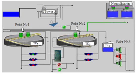
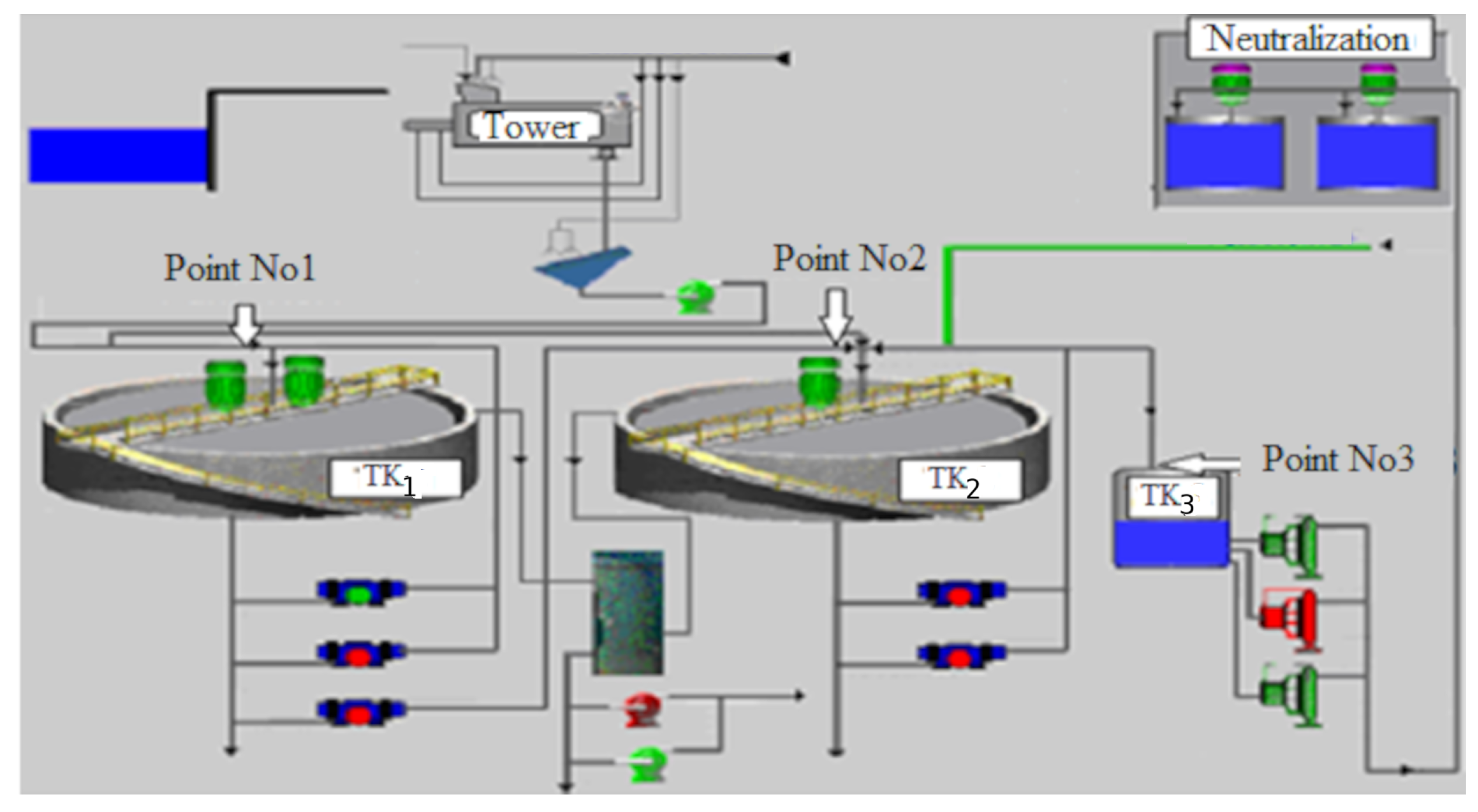
We collected samples of pulps from three different sites at the preparation plant, as illustrated in Figure 1. The collection sites are indicated in this figure as $T{K}_1$, $T{K}_2$, and $T{K}_3$. As the fluid moves along the plant, the concentration of solid particles increases. Site $T{K}_1$ is located at the entrance of the preparation plant, while site $T{K}_3$ is located just before the exit, where the pumps move the substance to the section in which acid lixiviation process occurs. We collected overflowing water from the sedimentation tanks to modify the solid particle concentration of the samples collected at sites $T{K}_1$, $T{K}_2$, and $T{K}_3$. In this way, we could produce samples with solid particle contents in the range 17% to 50%. The second independent variable used was pH. This parameter is important for controlling the formation of particle aggregates in the suspension. Finally, the third independent variable was the polydispersity index. This parameter is hard to control; however, it is feasible to measure it and to evaluate its influence on the rheological behavior of carbonated slime pulps.

2.1. Equipment and Utensils

In this research, we measured the following: the concentration of solid particles, the pH, the polydispersity index, the shear rate, and the shear stress. The measurement of solid particle concentrations is a relatively simple task, requiring the measurement of the density of both the solid particles and water. The density of the solid particles was 2.56 g/cm³, whereas the water density was 0.9963 g/cm³. The concentration in weight C is defined as

$$C={\displaystyle \frac{m_s}{m_s+m_w}}\times 100\%$$

(3)

where $m_s$ is the mass of the solid particles, and $m_w$ is the mass of water in the suspension.

The second independent variable, pH, was measured via a pH meter. This device measures the potential difference between an electrode sensitive to hydrogen ions and a reference electrode. pH is important because it provides a means of estimating surface charges. The third independent variable was the polydispersity index, which measures particle size distribution (PSD). The polydispersity index is defined as the ratio of the standard deviation and the mean value of the particle size distribution. Finally, we used two different viscometers to measure the shear rate and the shear stress.

The equipment used for this research was as follows:

• A HAAKE VT 550 viscometer (Thermo Fisher Scientific, Karlsruhe, Germany);
• A Brookfield DVELV viscometer (AMETEK, Middleborough, MA, USA);
• A digital balance BSA 142S (Sartorius, Gottingen, Germany);
• A moisture balance (RADWAG Wagi Elektroniczne, Radom, Poland);
• A mechanical shaker with a mechanical impeller OS2O (DLAB Scientific Co., Ltd. Beijing, China);
• A pH meter PH211 (Termo Fisher Scientific, Karslruhe, Germany);
• An “Analysette 22” COMPACT laser particle sizer (Fritsch GmbH, Idar-Oberstein, Germany).

The HAAKE 550 viscotester is a Searle rotational viscometer. This device operates as a controlled shear rheometer; that is, the angular velocity is set, and then the shear stress is measured. It has been designed to measure the flow curves for liquids and semi-solid substances. To measure the flow properties of the pulps, we used an SV DIN probe. This probe is designed to measure the flow curves of water-based plastic dispersion and paints. Each sample was placed inside the viscometer. The measurement sequence began with a higher angular velocity, which then decreased linearly over time. The device converted data from angular velocity and torque to the shear rate and shear stress. At the end of the process, we obtained the flow curves and the apparent viscosity. The 550 HAAKE viscometer was used to obtain the flow curves for shear rates in the range 10 to 650 s⁻¹. As the SV DIN probe has a smooth shearing surface, the determination of the flow curves is affected by the slip layer. To evaluate the influence of the slip layer on the measurement of the rheological properties of the substance, we used a Brookfield DVELV viscometer. This device allows for measuring the flow curves in the interval $0.06<\dot{\gamma }<20$, a range for which the slip becomes relevant. According to previous research [44,45], at low stresses, the slip prevents the correct measurement of the flow properties. On the contrary, at high stresses, the slip is present, but its influence is negligible, and, consequently, the rheological properties are correctly measured.

The “Analysette 22” COMPACT laser particle sizer measures the size of particles through an optical method. It contains a 635 nm laser diode with a power of less than 1 mW. This device uses laser light diffraction to measure the size of the particles. On one side, the deflection angle of the laser beam is inversely proportional to the particle size, and on the other side, the intensity of the diffracted laser beam is proportional to the number of particles. A convergent lens focuses the scattered light on the focal plane, where a detector measures the light energy distribution. Then, the particle size distribution is calculated from the data of the energy distribution using software called “Analysette 22 for Windows”. To determine the particle size, two models are used, namely the Diffraction Fraunhofer model and the Mie theory. The Fraunhofer diffraction is suitable for particles with diameters greater than $10\lambda$ (6.35 $\mathsf{\mu }$m for our laser). The Mie theory (which involves solving the Maxwell equations) allows for determining the sizes of particles with diameters between 0.3 and 6.5 $\mathsf{\mu }$m. Using this apparatus, it is possible to determine the size of particles between 0.3 and 300 $\mathsf{\mu }$m, a range sufficient to characterize the suspension investigated. The methodology used to measure the size distribution of the solid particles is defined as follows: We took a sample of the solid particles from the substance, typically 1–3 g. Then, the sample was put into the fluid reservoir. To disaggregate and disperse the particles into the water, we used an ultrasonic bath and a stirrer. To move the particles into the measuring unit, a centrifugal pump was used. The scatter produced by the particles was recorded via the detector, and then the data were processed to evaluate the particle size distribution. The measurement typically requires less than 1 min to complete.

Otherwise, we used the following equipment:

• A 500 mL graduated cylinder of 500 mL;
• 500 mL beakers;
• 20 L containers;
• 20 mL syringes;
• 250 mL glass jars.

The 20 L containers were used to collect samples of carbonated slime at points $T{K}_1$, $T{K}_2$ and $T{K}_3$. The other items were used to prepare the samples used in the experiments as described in the following subsection.

2.2. Preparation of the Mineral Suspensions

We collected 9 samples of carbonated slime pulps in 20-L containers from three different places in the preparation plant. In

Table 1. The carbonated slime pulp was collected from three different places. At each point, three different samples were taken (labeled from MC1 to MC9). In this table, the concentrations of solid particles are indicated and lie between 18.51% and 46.54%.

Sampling Point	Sample Label	Concentration of Solid Particles %
Point $T{K}_1$	MC1	18.51
	MC2	24.37
	MC3	21.58
Point $T{K}_2$	MC4	33.61
	MC5	38.13
	MC6	36.23
Point $T{K}_3$	MC7	38.94
	MC8	41.28
	MC9	46.54

, we summarize the concentration of solid particles in each sample. The next step was preparing 200 g samples with concentrations in the range 17% to 50%. For each concentration, we prepared three samples.

To produce samples of a given concentration, we needed to modify the initial concentration of one sample. We proceeded as follows: Sample MC9, picked at position $T{K}_3$, was used to prepare a suspension with a concentration of 50%. This concentration was attained via the following process: The sample was kept at rest for 30 min until solid particles settled. Then, water was extracted from the top with a syringe until the concentration increased to the desired value. In contrast, to produce samples with concentrations between 40% and 45%, we used samples MC8 and MC9. To increase the concentration of sample MC8, we used the previously described settling process, and to reduce the concentration of sample MC9, we added overflowing water. To produce samples with concentrations in the interval 30–35%, we used sample MC6, collected at point $T{K}_2$. The original concentration of this sample was 36.23%. The concentration of solid particles was reduced using overflowing water until the desired concentration was attained. For the remaining concentrations, we used samples MC1 to MC4.

2.3. Least-Squares Regression

For each sample, we obtained a flow curve. The data of ${\tau }_i$ and $\dot{{\gamma }_i}$ were then adjusted to the Herschel–Bulkley model using least-squares fitting. The regression provided the following parameters:

• ${\tau }_0$: yield stress;
• K: consistency index;
• n: flow index.

To obtain these parameters from an experiment with m pairs of data ($\dot{{\gamma }_i},{\tau }_i$), we need to minimize the following:

$$L=\sum _{i=1}^m{\left({\tau }_0+K{\dot{\gamma }}_i^n-{\tau }_i\right)}^2$$

(4)

The main difficulty in performing least-squares fitting comes from the fact that, although the yield stress ${\tau }_0$ and consistency index K are linear terms, the flow index is an exponent. For this reason, least-squares fitting must be performed using a numerical procedure such as the Gauss–Newton method [46]. In this study, we chose the following procedure: We set a value of n, so the model became linear with the remaining parameters. Then, we performed a linear regression to compute ${\tau }_0$ and K, and we evaluated the corresponding correlation coefficient R(n). We repeated this procedure for a set of ns between 0 and 1; the values are given by $n_j=j{\delta }_0$, where j = 1, …, 1000 and ${\delta }_0=0.001$. The choice of this interval was based on the assumption that the fluid is shear-thinning. We selected the value of $n_j$ for which the correlation coefficient had the maximum value (hereafter, we call this $N_1$). We assumed that $R_1=R\left(N_1\right)$. The following step was taken to consider a new interval [$N_1-{\delta }_0$, $N_1+{\delta }_0$]. In this new interval, we calculated the correlation coefficient for a new set of ns for which the increment was ${\delta }_1={\delta }_0/1000$. We retained the new value for which the correlation coefficient was maximum (we called this value $N_2$) and the corresponding correlation coefficient $R_2=R\left(N_2\right)$. We continued with this process until $\parallel R_p-R_{p-1}\parallel <ϵ$, where $ϵ$ is small enough, for instance, $ϵ={10}^{-9}$. A second method used for performing least-squares fitting is a procedure proposed by Mullinex [47]. Mullinex defines a function $\overline{F}\left(n\right)$ (which is a determinant) whose root gives the value of n. After obtaining n, the fitting of the yield stress ${\tau }_0$ and the consistency index K can be achieved by solving the equations of a linear regression, which is straightforward. The values obtained for ${\tau }_0$, K, and s are essentially the same for both procedures.

To build an empirical model of the rheological behavior of the pulps, we investigated the dependence of the parameters ${\tau }_0$, K, and s with respect to C, pH and s. We proposed a set of formulas to approximate these parameters based on the experimental data and previous studies. We considered the research of L. Pérez on the rheological properties of lateritic suspensions [27,34,36]. In the model, we included linear terms and products of the independent variables. We also included powers of s to fit K to the experimental data. The general form of the formulas of the model is

$$\begin{array}{c}\hfill P=a_0+a_1\times s+a_2\times C+a_3\times pH+a_4\times pH\times C+a_5\times pH\times s+a_6\times s\times C\\ \hfill +a_7\times s^{0.25}+a_8\times s^{0.45}+a_9\times s^{0.65}\end{array}$$

(5)

where P stands for ${\tau }_0$, K, or n. For ${\tau }_0$ and n, $a_7=a_8=a_9=0$. The constants appearing in Equation (5) were obtained through non-linear regression using a procedure similar to that for fitting the experimental data to the Herschet–Bulkley model. The correlation coefficient R of these equations was greater than 0.95 in all cases.

One of the main contributions of this study is its evaluation of the influence of pH on the rheological properties of carbonated slime pulps. Until now, very few studies have been conducted on this topic. In the studies of G. Hernandez et al. [48], L. Perez [34], and L. Perez and I. Garcell [35], the influence of pH is investigated but only in a narrow range. In contrast, we investigate the behavior of the rheological parameters of carbonated slime pulps over an extended range of concentrations C, a task that has not been carried out before. Finally, we take into account the influence of particle size distribution.

3. Rheological Measurements

The flow curves were obtained via two rotary viscometers (the characteristics of these devices are mentioned in Section 2.1). Regarding the Haake 550 viscometer for each value of the shear rate, we repeated the measurement of shear stress three times. From the data, we calculated the arithmetic mean, standard deviation $\sigma$, and coefficient of variation. In Appendix A, we show a table containing the results of the shear rate and shear stress measurements in a sample with the following values of independent variables: s = 0.713, C = 17%, and pH = 7.71. In all cases, the coefficient of variation was less than 1%. Similar results were obtained for the other samples, so we can state that the measurements are reproducible. A different procedure was followed for measurements performed using the Brookfleid viscometer. Because, at low values of $\dot{\gamma }$, the data of shear stress exhibit a high variance, we decided to repeat each measurement 10 times. The reported value of $\sigma$ is the arithmetic mean of these ten measurements.

As mentioned before, to measure the shear stress at low values of $\dot{\gamma }$, we used a Brookfield DVELV viscometer. We used this device for two reasons: Firstly, we used it to obtain a better estimate of the yield stress, and secondly, this viscometer has been used to evaluate the influence of the slip layer on the measurement of the rheological properties of the substance. Regarding the second reason, we performed two kind of measurements. In the first one, the slip was suppressed by sticking a sandpaper sheet on the spindle’s surface, as proposed in previous studies [49]. In the second case, the experiments were performed using a smooth shearing surface to allow the formation of the slip layer.

The data obtained in experiments with the rough surface need to be corrected because the dimension of the spindle increases as a result of the presence of the sandpaper. Using a viscometer, the shear stress is calculated from the torque exerted on the spindle. The relation between the torque M and the shear stress $\tau$ is

$$M=\tau Sr$$

(6)

where S is the shearing surface, and r is the spindle’s radius. In a cylindrical spindle, $S=2\pi rH$, where H is the height of the shearing surface. The sandpaper increases the spindle radius by $\Delta r=0.45$ mm. Then, the shear stress is calculated according to the following relation:

$$\tau ={\displaystyle \frac{M}{2\pi H{(r+\Delta r)}^2}}={\displaystyle \frac{M}{2\pi H{r}^2}}{\displaystyle \frac{1}{{(1+\Delta r/r)}^2}}$$

(7)

As the spindle’s radius increases due to the influence of the sandpaper, the value of the shear stress given by the viscometer must be multiplied by the factor ${\displaystyle \frac{1}{(1+\Delta r/r)2}}$.

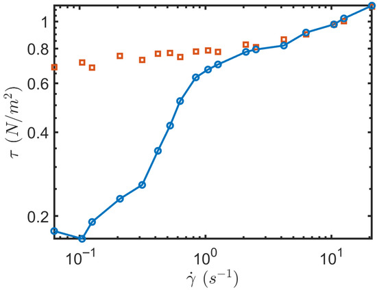
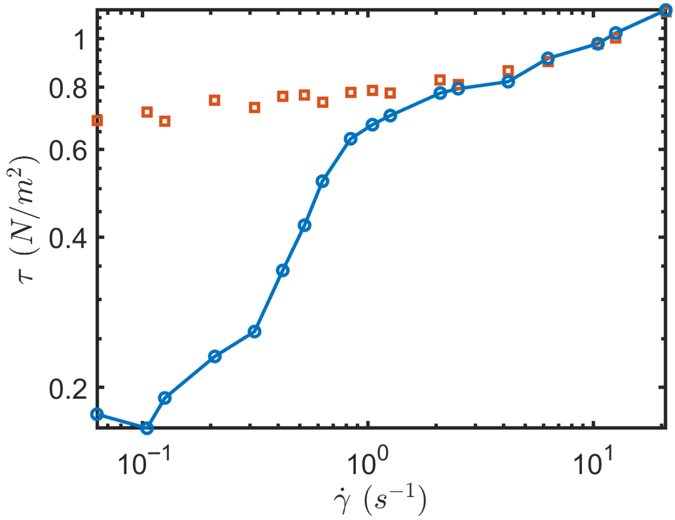
To illustrate the influence of the slip layer on the measurements of the rheological properties of the substance, in Figure 2, we present the flow curves obtained, respectively, using a rough surface and a smooth surface for a fluid with the solid particle concetration C = 20%. We observe that, when $\dot{\gamma }\to 0$, the experimental data provide different estimates of the yield stress. The slip layer leads to the underestimation of ${\tau }_0$ by a factor approximately 4. Both curves approach each other as $\dot{\gamma }$ increases. The curve obtained using the smooth shearing surface displays a kink after both curves coincide. The value of the shear rate for which the kink occurs depends on the concentration, but in any case, it is less than 15 s⁻¹. This feature is proof that most of the data taken using the Haake viscometer correctly reproduce the flow properties of the substance.

3.1. Flow Curves for Different Solid Particle Concentrations

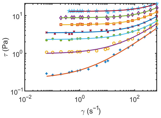
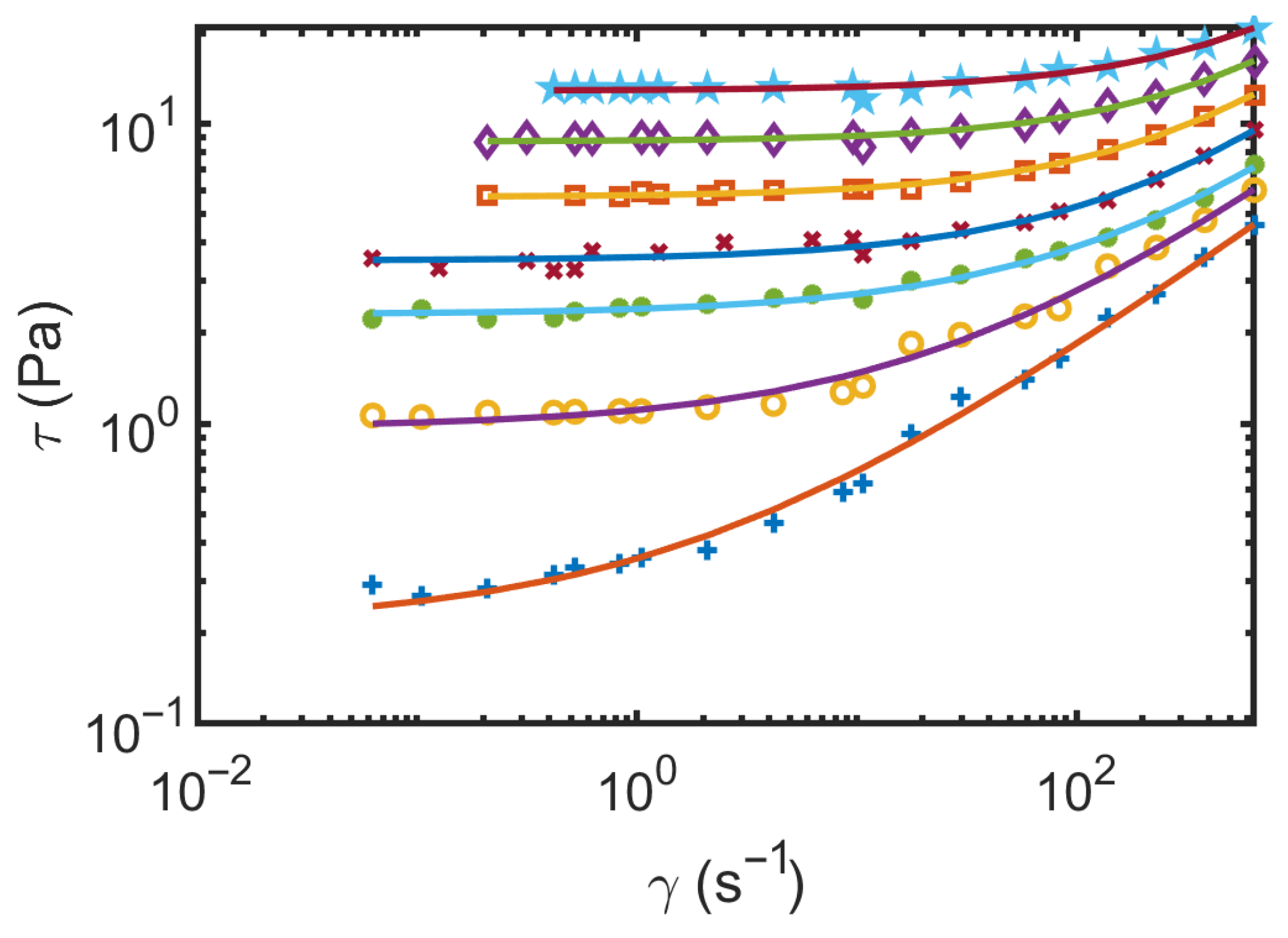
We performed measurements of $\tau$ and $\dot{\gamma }$ to obtain the flow curves of carbonated slime pulps for the following values of C at a temperature of 28 °C: 17%, 24%, 30%, 35%, 40%, 45%, and 50%. The temperature was measured during the experiments using a Pt-100 probe. In all measurements, the value of pH lies in the range from 7.71 to 8.52. In Figure 3, we present flow curves for pH = 8.14. The curves in this figure exhibit behavior typical of viscoplastic suspensions, that is, a non-linear relationship between the two variables, and the existence of a yield point. For a fixed value of the shear rate ($\dot{\gamma }$), the greater the concentration of solid particles, the greater the shear stress ($\tau$). This behavior reflects the fact that the content of solid particles has an important influence on the rheological properties of the substance. The flow curves shown in Figure 3 were fitted to the Herschel–Bulkley model using the procedure outlined in Section 2. In

Table 2. The rheological parameters that appear in the Herschel–Bulkley model for the carbonated slime pulps when temperature $T=28 °$C for different concentrations of solid particles. The value of pH is 8.14.

Concentration of the Solid Particles (%)	${\mathit{\tau }}_0$	K	n	R
17	0.2138	0.1415	0.531	0.9979
24	0.9694	0.1395	0.555	0.9942
30	2.3126	0.0959	0.606	0.9922
35	3.4930	0.0870	0.654	0.9906
40	5.6827	0.0811	0.685	0.9984
45	8.6986	0.0749	0.713	0.9964
50	12.8495	0.0724	0.726	0.9956

, we present the parameters that appear in the model, namely the yield stress (${\tau }_0$), the consistency coefficient K, and the flow index n. The yield point and the flow index increase with the concentration, whereas K decreases.

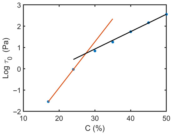
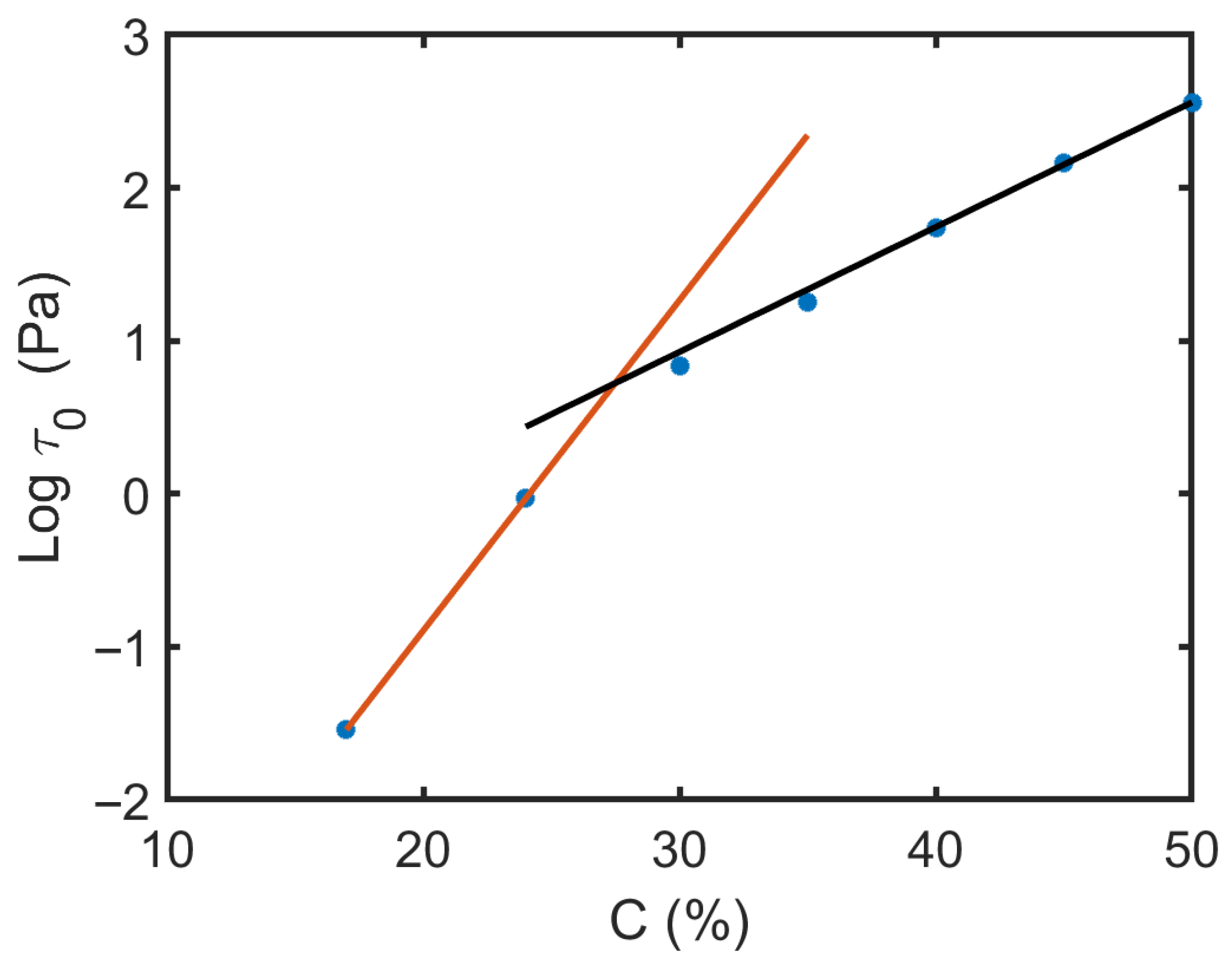
To highlight the modifications to the rheological properties that occur as the concentration increases, we plotted in Figure 4 the yield stress vs. C for the data in the previous figure. The data are shown in semi-log scale. In the figure, we observe two different behaviors, one for C < 25% (red line) and the other for C > 40% (black line). Similar behavior has been observed in previous research on viscoplastic fluids.

3.2. Effect of pH on the Rheological Behavior of the Pulps

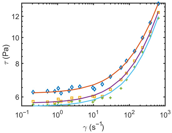
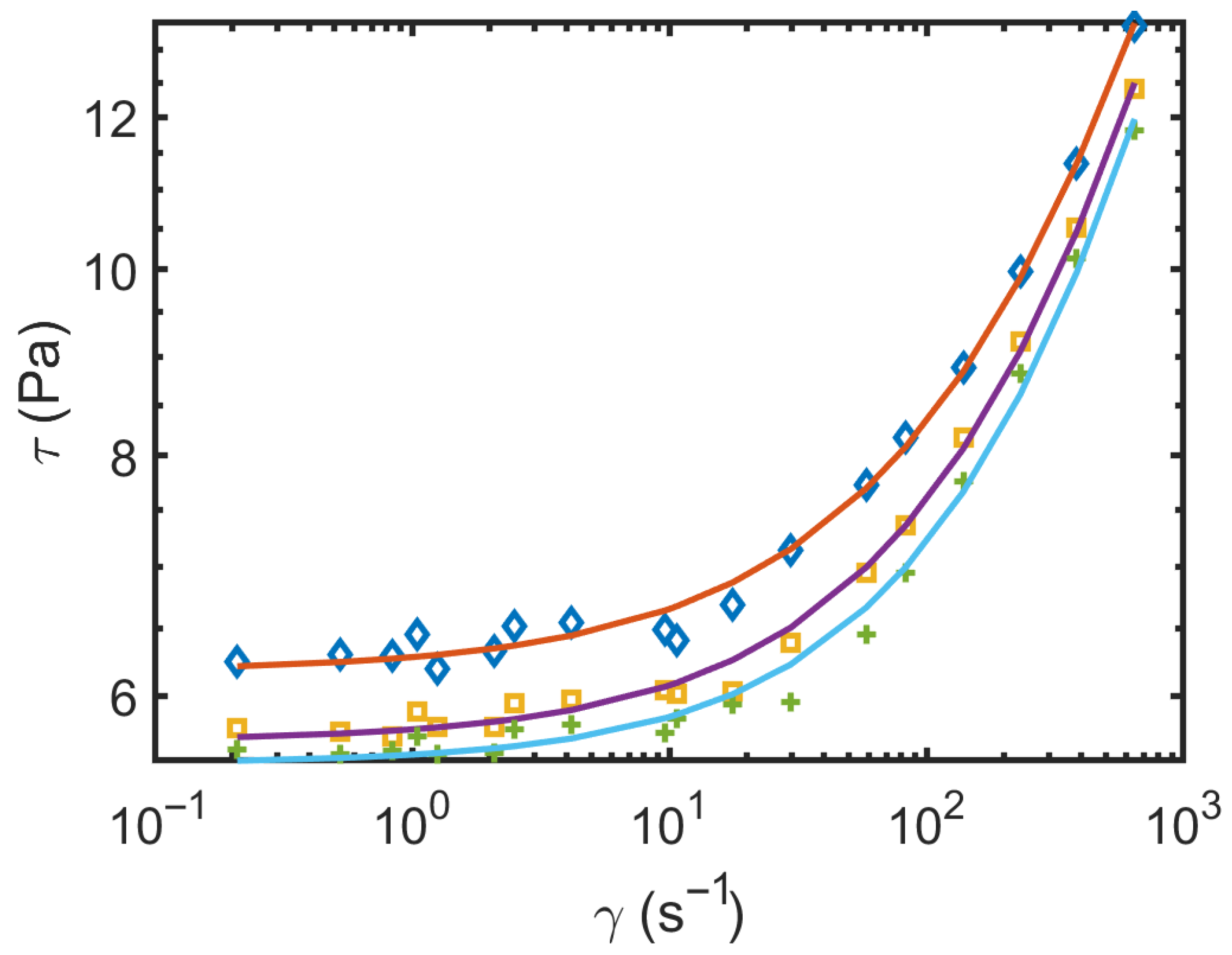
pH is a variable used to measure the acidity of a solution. This variable is related to factors such as the surface charge density, point of zero charge (p.z.c.), and electrokinetic potential. If we consider that the dispersed phase in a suspension has a large surface area and that the surface’s charge affects the formation of aggregates, it is easy to understand that the rheological behavior of the carbonated slime pulps depends on the pH value. This dependence has previously been reported by Garcell [31], Kosmulski [50,51] and Perez [36]. To exhibit the influence of pH on the rheological properties of carbonated slime pulps, in Figure 5, we plot flow curves corresponding to three different values of pH, namely 7.71, 8.14, and 8.52. As in Figure 3, the three curves display a non-linear relationship between $\tau$ and $\dot{\gamma }$, and there is a yield point. In this respect, for pH = 8.52, ${\tau }_0=5.5318$ (blue line), whereas for pH = 7.71, ${\tau }_0=6.1777$ (red line). This figure shows that for a fixed value of $\dot{\gamma }$, the greater the pH, the lower the shear stress.

The data of the flow curves shown in Figure 5 are fitted to Equation (2). The results are shown in

Table 3. Fitting between the shear stress $\tau$ and shear rate $\dot{\gamma }$ for different pH values. The data are adjusted to the Herschel–Bulkley model. The solid particle concentration is 40%.

pH	Adjusted Model	${\mathit{R}}^2$
7.71	$\tau =6.1777+0.1068{\dot{\gamma }}^{0.651}$	0.9981
8.14	$\tau =5.6827+0.0811{\dot{\gamma }}^{0.685}$	0.9984
8.52	$\tau =5.5318+0.0603{\dot{\gamma }}^{0.764}$	0.9981

, where we present the resulting equation and the regression coefficient R of the fitting. As shown, the correlation coefficient is always greater than 0.997, which indicates good agreement between the model and the experimental data.

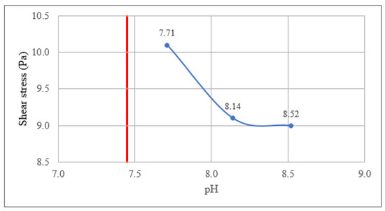
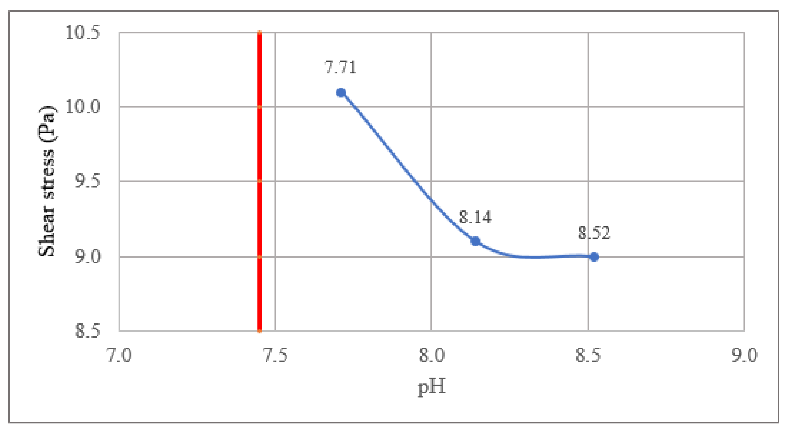
The stability of the carbonated slime pulps must be considered when the rheological properties are investigated. This stability depends on the proximity of the pH to the point of zero charge (p.z.c.). The p.z.c. is the value of the pH at which the surface charge vanishes. For the substance investigated, p.z.c. = 7.41. For pH values far from the p.z.c., the solid particles have a greater surface charge, so electrostatic forces prevail. Under these circumstances, sedimentation is almost non-existent, and, consequently, the suspension is stable. On the contrary, for pH values near the p.z.c., the surface charge decreases; then, the attractive forces become dominant. The suspension becomes unstable because the particles tend to form flocculi and aggregates. Under these circumstances, the suspension can settle, as reported by Beaton [52], Cardero [53], and Pérez-Garcia [36].

To highlight the importance of pH on the rheological behavior of carbonated slime pulps, in Figure 6, we plotted the shear stress as a function of pH for a given value of $\dot{\gamma }$ and C = 40%. The point of zero charge corresponds to the red vertical line. In this figure, we can see that the shear stress increases as the pH approaches the p.z.c., reaching a maximum value (among the data plotted) when pH = 7.71. It is expected that the maximum apparent viscosity is attained around the p.z.c., in agreement with the results obtained by Perez [36] and Hernandez [54]. The increase in shear stress when $\tau \to p.z.c$ reflects the fact that the attractive forces become dominant, so the particles form clusters and the suspension becomes unstable; then, the suspension acquires viscoplastic properties. On the contrary, for pH values far from the p.z.c., the repulsive forces become dominant, inhibiting cluster formation, and the shear stress decreases. For pH > 8.30, the shear stress remains nearly constant. The strong increase in shear stress as $pH\to p.z.c$ and the constant value of $\tau$ for pH > 8.3 were considered when building the empirical model.

3.3. Granulometric Analysis of the Samples

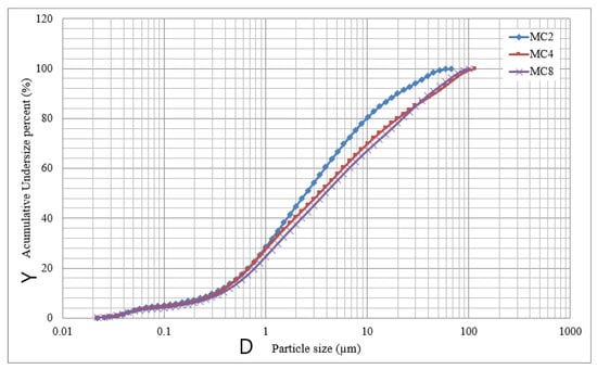
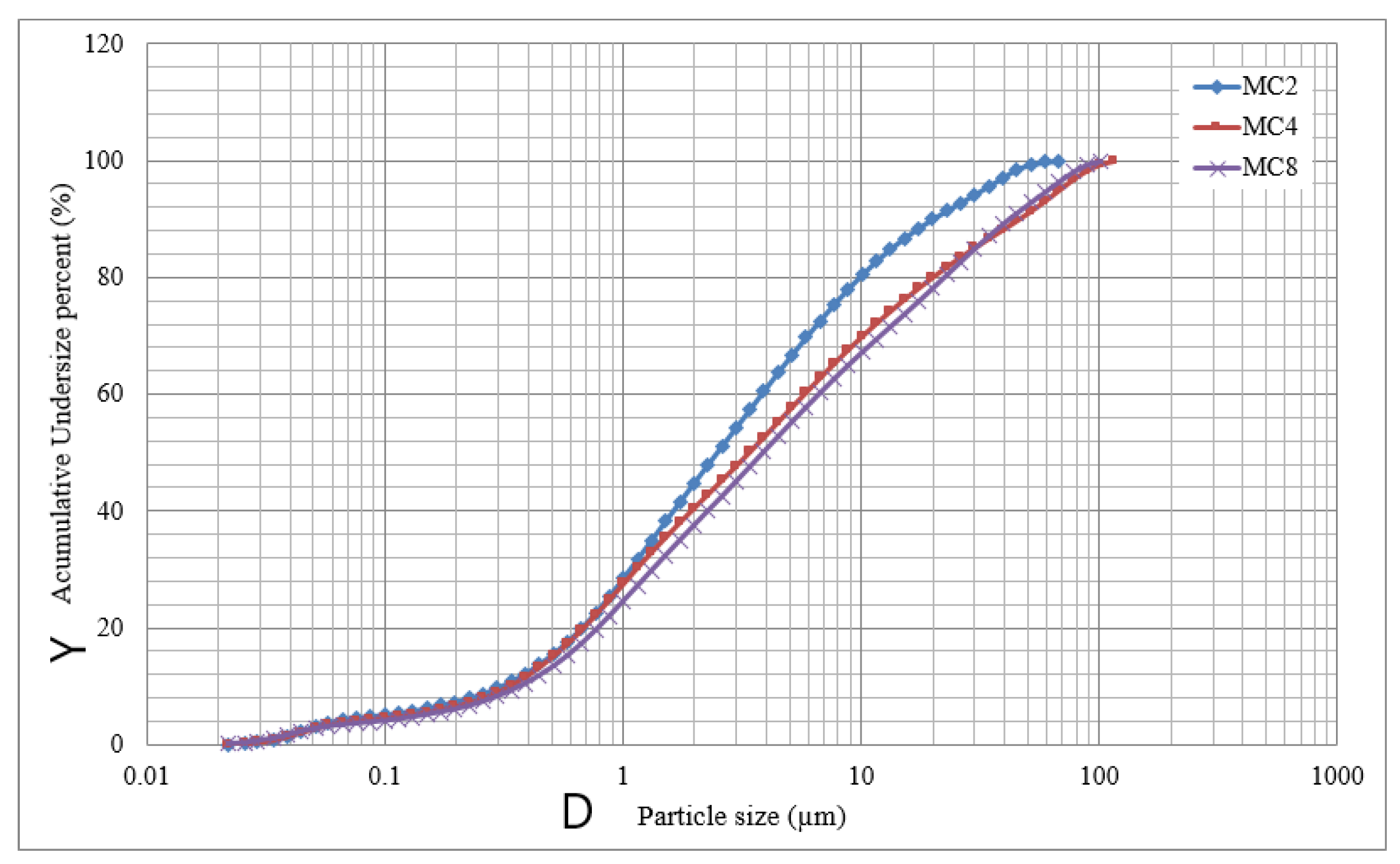
The size of the solid particles affects the rheological properties of the pulps because electrical charges can be present on the surface. To understand the importance of particle size distribution, recall that for a particle of diameter d, the quotient of area to volume is proportional to 1/d. Then, fine particles can contain more surface charges than coarse particles. To measure the diameter distribution of particles, we used an “Analysette 22 COMPACT” Particle Sizer. Using this device, it is possible to determine the fraction of particles smaller than 45 $\mathsf{\mu }$m, a task that cannot be completed with sieves. One parameter used to measure the degree of polydispersity is particle size distribution (PSD), defined as the probability density function of the particle size. However, in most studies on suspensions, another parameter is used: the fraction of particles (Y) with a diameter less than D. These parameters are related because Y is the integral from 0 to D of the PSD.

A Laser Particle Analyzer was used to determine the particle size distribution and Y(D) for all the samples. In Figure 7, we plot Y vs. D for three samples, namely MC2, MC4, and MC8. The curves of the remaining samples exhibit a similar trend. The results in this figure show that in the carbonated slime pulps, most particles are smaller than 100 $\mathsf{\mu }$m. The median of their size distribution $D_{50}$ lies around 5 $\mathsf{\mu }$m. Based on the results in this figure, we conclude that the samples comprise silt, clay, and fine sand. This particle size distribution provides plastic properties to the suspension, which is typical of polydisperse systems, as reported by Perez-Garcia [36] and Hernandez et al. [55].

The polydispersity index s can be computed directly from the experimental data obtained using the laser particle sizer. Another means of determining s is by using a model of the granulometric distribution proposed by L. Perez [36,54]. This model has been successfully tested in lateritic suspensions and carbonated slime pulps [55]. The equation of this model is

$$Y_N={\left({\displaystyle \frac{D_N}{(1-B_N)D_N+B_N}}\right)}^s$$

(8)

In this equation, $D_N$ is the normalized diameter $D/D_{50}$, where $D_{50}$ is the median of the particle size distribution, and $Y_N$ is the normalized fraction $Y/Y_{50}$. $B_N$ is a free parameter obtained from least-squares regression. The polydispersity index is an exponent in this equation. The results presented here were fitted to the model of granulometric distribution. In

Table 4. The coefficients of the model of the distribution of particle sizes and the polydispersity index.

Sample	${\mathit{D}}_{50}$	${\mathit{B}}_{\mathit{N}}$	s	${\mathit{R}}^2$
MC2	34.255	0.601	0.749	0.9980
MC4	26.111	0.582	0.765	0.9981
MC8	19.904	0.512	0.976	0.9996

, we present the results for fitting this model using three different samples. In this table, we show the parameters that appear in Equation (8) and the polydispersity index s.

4. Empirical Model to Predict the Rheological Parameters

The flow curves shown in Figure 3 and Figure 5 were fitted to the Herschel–Bulkey model. The correlation coefficients of the regressions were greater than 0.997 in all cases, reflecting good agreement between the data and the model. Other data not presented here were also adjusted to Equation (2). From all the experimental data, we built an empirical model relating ${\tau }_0$, K, and n to the independent variables C, pH, and s. To do this, we calculated the values of ${\tau }_0$, K, and n for all the flow curves. We used a set of the dependent variables as functions of C, pH, and s. The data were fitted to Equations (9)–(11) to obtain constant appearance in these formulas. In proposing this model, we consider the following: (a) the concentration C has a strong influence on the rheological properties of the substance; (b) the shear stress grows rapidly as $pH\to p.z.c$ and attains an asymptotic value for pH > 8.3. The formulas include linear and interaction terms (products of the independent variables). The constants of the formulas of our model were computed through a non-linear regression. The formulas for the yield point, the consistency coefficient, and the flow index resulting from the regression are as follows:

For the yield stress ${\tau }_0$,

$$\begin{array}{c}\hfill {\tau }_0=11.734-24.259\times s-0.17124\times C-0.10854\times pH+1.0253\times s\times C\\ \hfill -0.05679\times C\times pH+0.86935\times s\times pH{R}^2=0.998\end{array}$$

(9)

For the consistency index K,

$$\begin{array}{c}\hfill K=6085.74+3549.38\times s-0.002667\times C-0.51637\times pH+0.50895\times s\times pH\\ \hfill -30726.16\times s^{0.25}+47905.11\times s^{0.45}-26813.80\times s^{0.65}{R}^2=0.979\end{array}$$

(10)

For the flow index n,

$$\begin{array}{c}\hfill n=-0.64571-0.17309\times s+0.008140\times C+0.14172\times pH{R}^2=0.987\end{array}$$

(11)

5. Validation of the Model and Application to Flow in Pipes

In the previous section, we presented an empirical model designed to estimate the rheological properties of the carbonated slime pulps. This model contains a set of equations for predicting the values of yield stress, the consistency index, and the flow index as a function of C, pH, and s. The concentration and the polydispersity index influence the rheological properties of the carbonated slime pulps. In the absence of solid particles, the fluid behaves in a Newtonian manner. When particles are added, the fluid acquires viscoplastic properties. Then, an increase in the particle concentration leads to an increase in the yield stress and the apparent viscosity. In contrast, the dependence of the rheological properties of the fluid on s is related to interparticle interactions and particle–fluid interactions. The intensity of these interactions is dependent upon the size of particles. Regarding the influence of pH on the rheological properties, further information is provided in Section 3.

5.1. Validation of the Model

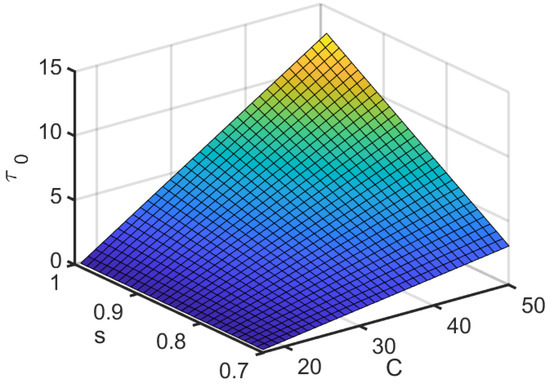
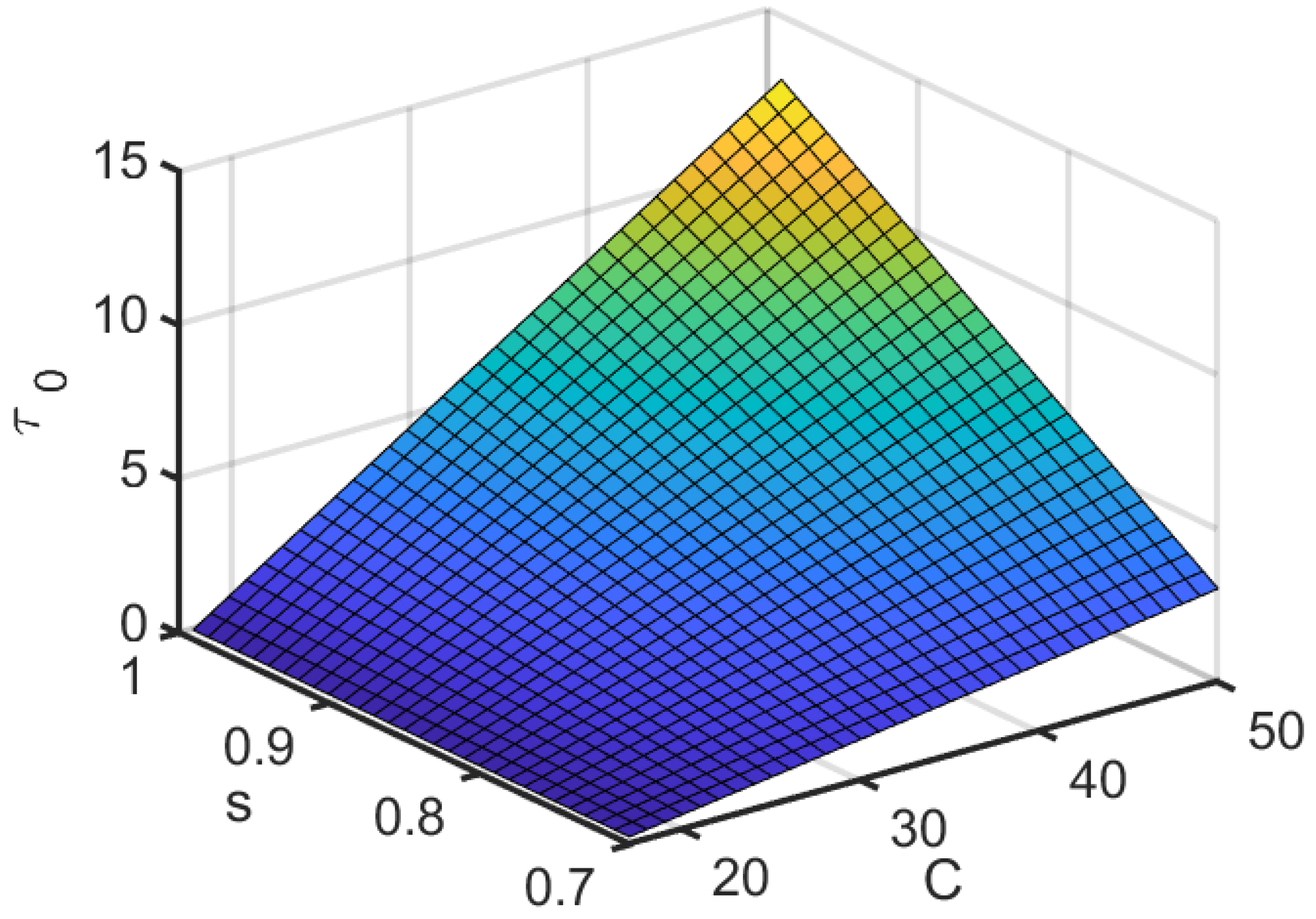
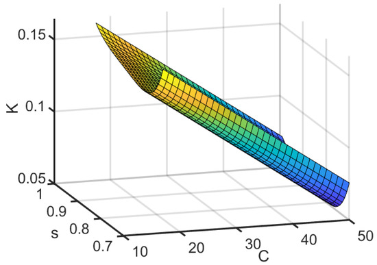
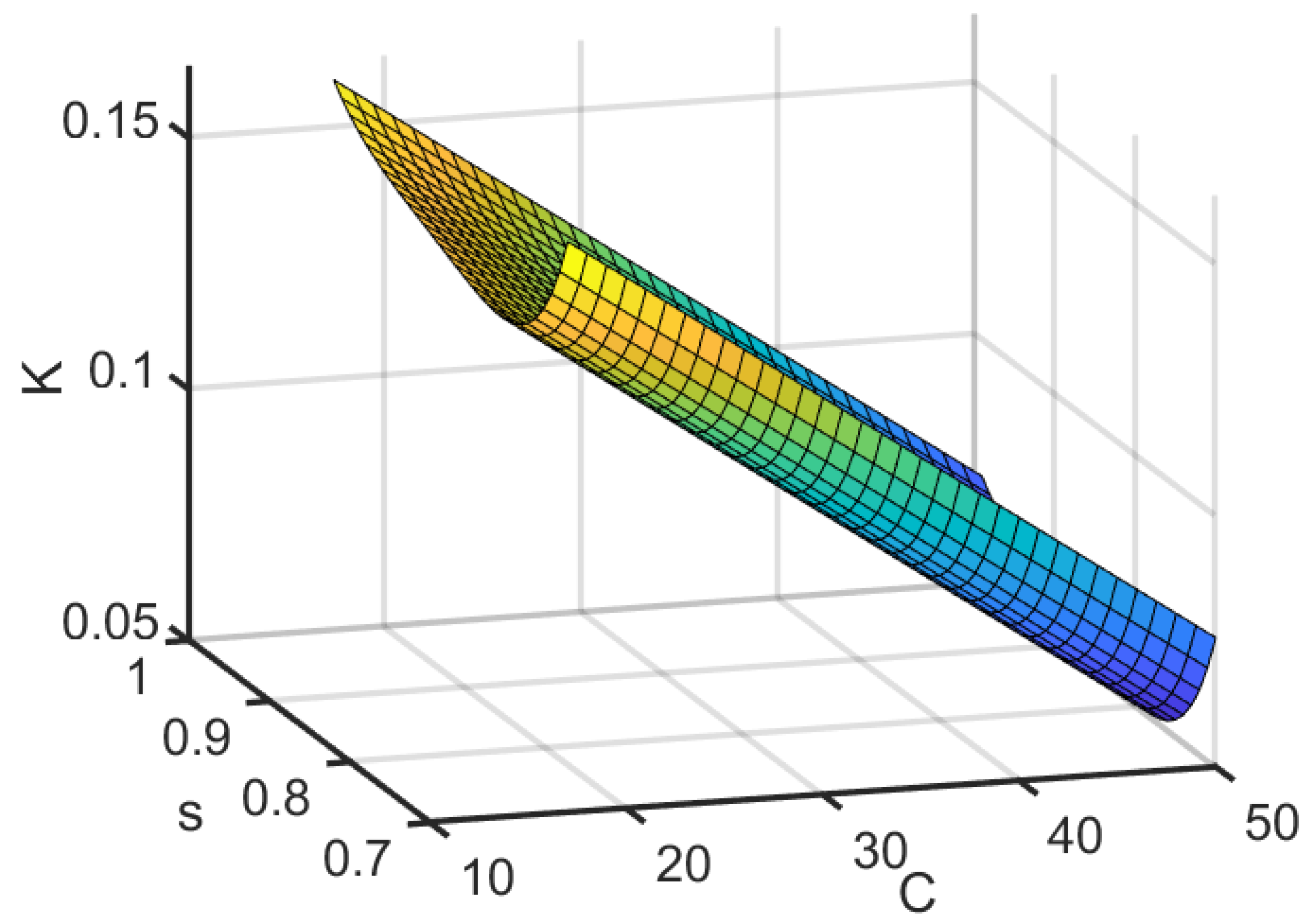
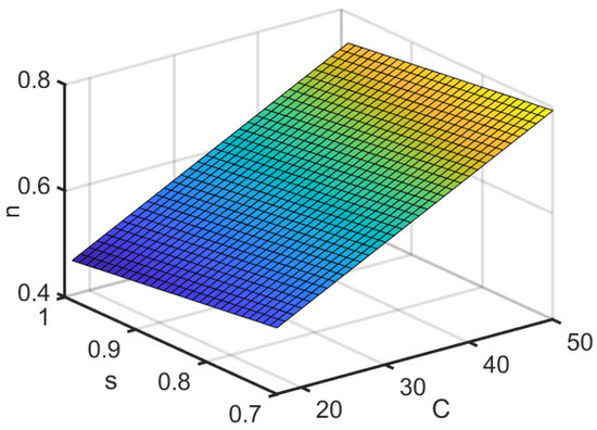
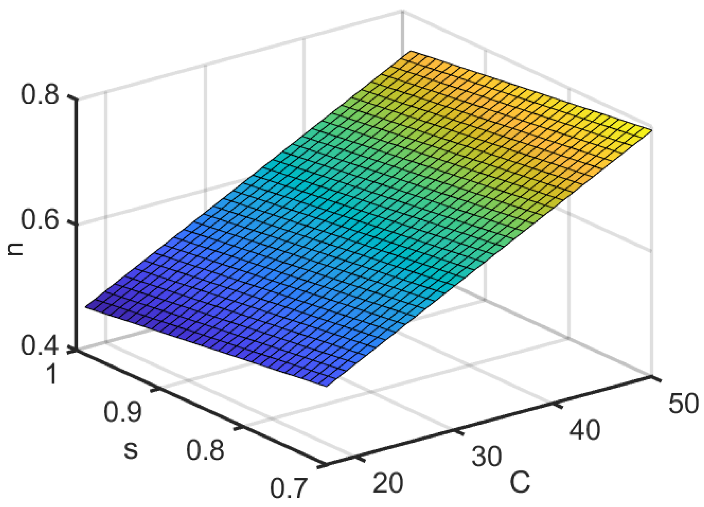
The following step involves validating the model under different experimental or operational conditions. We expect that ${\tau }_0$, K, and n will exhibit smooth dependence on the independent variables. To show that this trend is observed, in Figure 8, Figure 9 and Figure 10, we plot the parameters ${\tau }_0$, K, and n as functions of C and s for pH = 8.14.

According to Figure 8, the model predicts that yield stress lies in the range 0.2 to 12.9 Pa. The maximum value occurs when C = 50% and s = 0.98. The yield stress appears to be an increasing function of both the concentration C and the polydispersity index. This behavior is consistent with the experimental data presented in Figure 3 and Figure 5, where ${\tau }_0$ takes values between 0.22 and 12.85. With respect to the consistency index, the model predicts (see Figure 9) that K is a decreasing function of C and that the dependence on s is non-monotonic. The model predicts that K decreases as s increases when $0.7<s<0.78$. Beyond this range, the parameter K becomes an increasing function of s. Now, we turn our attention to the flow index n. According to the model, the flow index is an increasing function of C and a decreasing function of s. The model predicts that $n<1$, meaning that the carbonated slime pulps are thinning fluids. This prediction is corroborated by the experimental data.

The formulas of the model were tested for different values of C, K, and s. First, we took a flow curve related to all our data. Then, we performed a least-square regression to obtain the values of ${\tau }_0$, K, and n. These values were compared with the results given by Equations (9)–(11). This process was repeated for different sets of ($\tau$,$\dot{\gamma }$). The discrepancies between the data and the prediction were lower than 2% in all cases. For example, in

Table 5. A comparison between the model and the experimental data.

Variable	${\mathit{\tau }}_0$	K	n
Experimental	5.6827	0.0811	0.685
Model	5.6699	0.0813	0.687
Error (%)	0.22	0.25	0.29

, we compare the values of the apparent viscosity, yield stress ${\tau }_0$, K, and n obtained via the model and the experimental data. The values of independent variables are $s=0.846$, $C=40\%$, and $pH=8.14$. The discrepancy for the yield point is 0.22%, and for the other parameters, the difference is smaller than 1% It is important to remark that the model describes the rheological properties of the carbonated slime pulps in the following domains: $17\%\le C\le 50\%$, $0.717\le s\le 0.985$, and $7.71\le$ pH $\le 8.52$. The application of this model beyond these domains leads to important errors. Finally, the equations do not reproduce the experimental data when the independent variables are outside of the interval where fitting is performed, and in certain cases, the results are not consistent.

The mean value of the shear rate during the transport of carbonated slime pulps in the plant is 83.33 s⁻¹. According to the model, the apparent viscosity lies in the range 0.02 to 0.18 $\mathrm{N}\mathrm{ṡ}$/m² depending on the values of the independent variables.

5.2. Pressure Gradient and Hydraulic Power in a Pipeline

In a pipeline, the relation between the wall shear stress and the pressure gradient is as follows [56]:

$${\tau }_w={\displaystyle \frac{\Delta P}{\Delta L}}{\displaystyle \frac{D}{4}}$$

(12)

where D is the pipeline interior diameter. This relation is valid no matter the kind of fluid. For a Newtonian fluid and a turbulent flow, it is common to use the Darcy–Weisbach formula for the wall stress and the mean velocity V:

$${\tau }_w=f{\displaystyle \frac{\rho V^2}{8}}$$

(13)

where f is the friction factor. We can evaluate this quantity using the following equation:

$$\sqrt{{\displaystyle \frac{8}{f}}}=2.5ln\left(Re\sqrt{{\displaystyle \frac{f}{8}}}\right)$$

(14)

For a fluid satisfying the Herschel–Bulkley model in the laminar regime, the pressure gradient is

$${\displaystyle \frac{\Delta P}{\Delta L}}={\displaystyle \frac{4}{D}}\left[{\tau }_0+K{\left({\displaystyle \frac{3n+1}{4n}}\right)}^n{\left({\displaystyle \frac{32Q}{\pi D^3}}\right)}^n\right]$$

(15)

where Q is the volumetric flow rate. For a turbulent flow, which is the case for most industrial applications, the pressure gradient in a suspension has three contributions: (a) A pressure loss related to gravity, which is equal to $\rho gsin\left(\theta \right)$, where $\theta$ is the pipe inclination angle. Then, for a horizontal pipeline, this term vanishes. (b) The second contribution is related to the shear stress in the wall. The wall stress in the Herschel–Bulkley model is

$${\tau }_w={\tau }_0+K\left({\displaystyle \frac{32Q}{\pi D^3}}\right){\left({\displaystyle \frac{3n+1}{4n}}\right)}^n\left[1-{\left({\displaystyle \frac{{\tau }_0}{{\tau }_w}}\right)}^{{\displaystyle \frac{n+1}{n}}}\right]$$

(16)

To obtain ${\tau }_w$, the previous equation must be solved via a numerical method. Moreover, (c) the third contribution is associated with mixing into the fluid. The solid particles in the suspension induce local vorticity and additional stresses. These factors modify the velocity profile and are responsible for additional energy dissipation. At present, we are developing a model to incorporate this third contribution based on dimensional analysis and experimental data. The pressure gradient in Herschel–Bulkley fluid is then modeled via the following equation:

$${\displaystyle \frac{\Delta P}{\delta L}}=\rho gsin\left(\theta \right)+{\displaystyle \frac{4{\tau }_w}{D}}+F(Re,C,s){\displaystyle \frac{\rho V^2}{D}}$$

(17)

where F is a function of the Reynolds number, the concentration C, and the polydispersity index s. To evaluate this gradient, we need to recognize the rheological parameters appearing in the Herschey–Bulkley model.

Finally, to evaluate the hydraulic power $P_H$, we use the following relation:

$$P_H=QL{\displaystyle \frac{\Delta P}{\Delta L}}$$

(18)

6. Conclusions

In this study, we built an empirical model of the rheological properties of carbonated slime pulps. We measured their flow properties as a function of the concentration of solid particles, pH, and the polydispersity index. As the shear rates involved in the experiments cover more than two orders of magnitude, the flow curves were fitted to the Herschel–Bulkley model. An important contribution of this study is the measurement of the rheological properties of carbonated slime pulps over varied operating conditions, a task that has not previously been performed. We observed a transition in the rheological properties as the concentration of solid particles grew. Additionally, we investigated the influence of pH, showing that, as pH increases, the rheological properties of the pulps exhibit asymptotic behavior. From our experimental data, we built an empirical model to predict the yield stress, the consistency index, and the flow index. The comparison between the experimental data and predictions of the empirical model gave errors of less than 4%. Our model can be used to improve the transport of carbonated slime pulps in the nickel industry and could be useful in other processes requiring the transport of mineral suspensions.

References

- Bingham, E.C. An investigation of the laws of the plastic flow. In US Bureau of Standards Bulletin; U.S. Government Printing Office: London, UK, 1917; Volume 13, pp. 309–353. [Google Scholar]
- Bingham, E.C. Fluidity and Plasticity, 1st ed.; Mc Graw Hill: New York, NY, USA, 1922; pp. 3–5. [Google Scholar]
- Coussot, P. Rheophysics. Matter in All Its States, 1st ed.; Springer: Cham, Switerland, 2014; pp. 188–190. [Google Scholar]
- Dey, L.; Jan, C.D.; Wang, J.S. Effect of particle fractions ob the Bingham yield stress and viscosity of fine-coarse particle suspensions. J. Mt. Sci. 2021, 18, 2960–2970. [Google Scholar]
- Wu, A. Rheology of Paste in Metal Mines, 1st ed.; Metallugical Industry Press and Springer: Beijing, China, 2022; pp. 42–43. [Google Scholar]
- Dinkgreve, M.; Paredes, J.; Denn, M.M.; Bonn, D. On different ways to measure “the” yield stress. J. Non-Newton. Fluid Mech. 2016, 238, 233–241. [Google Scholar] [CrossRef] [Scilit]
- Dzuy, N.Q.; Timothy, A.; Daniel, D.K.; Lixuan, Z. Yield stress measurements in suspensions: An inter-laboratory study. Korea-Aust. Rheol. J. 2006, 18, 15–24. [Google Scholar]
- Hsissou, R.; Hilali, M.; Dagdag, O.; Adder, F.; Elbachiri, A.; Rafik, M. Rheological behavior model of polymers. Biointerface Res. Appl. Chem. 2022, 12, 1263–1272. [Google Scholar]
- Caram, F.; Bautista, E.; Puig, O. On the rheological modeling of associative polymers. Rheol. Acta 2006, 46, 45–57. [Google Scholar] [CrossRef] [Scilit]
- Gomes, M.; Marchese, T. Ajuste de modelos reológicos mecânicos no creep de polipropileno, poliestireno e policarbonato: Comparação com o mef. Rev. Iberoam. Polim. 2013, 14, 65–83. [Google Scholar]
- Li, Z.; Wang, J.; Pérez-Camargo, R.; Müller, A.J.; Zhang, B.; Grayson, S.M.; Hu, W. Non-monotonic molecular weight dependence of crystallization rates of linear and cyclic poly(epsilon-caprolactone)s in a wide temperature range. Polym. Int. 2016, 65, 1074–1079. [Google Scholar] [CrossRef] [Scilit]
- McGuire, M.J.; Addai-Mensah, J.; Bremmell, K. The effect of polymer structure type, pH and shear on the interfacial chemistry, rheology and dewaterability of model iron oxide dispersions. Colloids Surf. Physicochem. Eng. Asp. 2006, 275, 153–160. [Google Scholar] [CrossRef] [Scilit]
- Mewis, J.; Frith, W.; Strivens, T.; Russel, W. The Rheology of Suspensions Containing Polymerically Stabilized Particles. AIChE J. 1989, 35, 415–422. [Google Scholar] [CrossRef] [Scilit]
- Briceño, M.; Salager, J.; Bertrand, J. Influence of the dispersed phase viscosity on the mixing of concentrated oil-in-water emulsions in the transition flow regime. In Proceedings of International Symposium on Mixing in Industrial Processes—ISMIP4, Toulouse, France, 14–16 May, 2001; pp. 286–292. [Google Scholar]
- Briceño, M.I.; Ramirez, M.; Bullón, J.; Salager, J. Customizing Drop Size Distribution to Change Emulsion Viscosity. In Proceeding of the 2nd World Congress on Emulsion CME2, Bordeaux, France, 23–26 September 1997. Paper 2-1-094. [Google Scholar]
- Ohtake, T.; Hano, K.; Takagi, F. Effects of viscosity on drop diameter of w/o emulsion dispersed in a stirred tank. J. Chem. Eng. Jpn. 1987, 20, 443–447. [Google Scholar] [CrossRef] [Scilit]
- Pal, R.; Masliyah, J. Rheology of oil in water emulsions with added solids. Can. J. Chem. Eng. 1990, 68, 24–28. [Google Scholar] [CrossRef] [Scilit]
- Rodríguez, T.H.; Angulo, H.J.; Falcón, J. Comportamiento reológico de las emulsiones empleando productos de la pirolisis. Tecnol. Quím. 2015, 35, 412–423. [Google Scholar]
- Vernáez, O.; García, A.; Castillo, F.; Ventresca, M.L.; Müller, A.J. Oil-based self-degradable gels as diverting agents for oil well operations. J. Pet. Sci. Eng. 2016, 146, 874–882. [Google Scholar] [CrossRef] [Scilit]
- Zen, G.K.; Zhu, Y.; Chen, W. A Brief Review of Micro-Particle Slurry Rheological Behavior in Grinding and Flotation for Enhancing Fine Mineral Processing Efficiency. Minerals 2023, 223, 792. [Google Scholar]
- Bekkour, K.M.; Leyama, A.; Benchabane, O. Time-dependent rheological behavior of bentonite suspensions: An experimental study. J. Rheol. 2005, 49, 1329–2345. [Google Scholar] [CrossRef] [Scilit]
- İşçi S, F.; Seniha Güner, Ö.; Güngör, N. Investigation of rheological and colloidal properties of bentonitic clay dispersion in the presence of a cationic surfactant. Prog. Org. Coat. 2005, 54, 28–33. [Google Scholar] [CrossRef] [Scilit]
- Blakey, B.C. Characterizing the rheology of laterite slurries. Int. J. Miner. Process 2003, 70, 23–39. [Google Scholar] [CrossRef] [Scilit]
- Bhattacharya, I.N.; Panda, P. Rheological behaviour of nickel laterite suspensions. Int. J. Miner. Process 1998, 53, 251–263. [Google Scholar] [CrossRef] [Scilit]
- Klein, A.; Hallbom, D. Modifying the rheology of nickel laterite suspensions. Miner. Eng. 2002, 15, 745–749. [Google Scholar] [CrossRef] [Scilit]
- Larson, R.G. The Structure and Rheology of Complex Fluids; Oxford University Press: New York, NY, USA, 1999. [Google Scholar]
- Pérez, L.; Garcell, L.; Rojas, A.; Simoes, R. Mineralogía y reología de suspensiones minerales del proceso de lixiviación ácida a presión en Moa. Min. Geol. 2010, 4, 16–35. [Google Scholar]
- Avramidis, S.; Turian, R.M. Yield Stress of Laterite Suspensions. J. Colloid Interface Sci. 1991, 143, 54–68. [Google Scholar] [CrossRef] [Scilit]
- Cerpa, A.; Garcell, L. Propiedades superficiales y reológicas de suspensiones minerales lateríticas. In Proceedings of the Metalurgia ’98, Havana, Cuba, 17–21 November 1998. [Google Scholar]
- Garcell, L.; Díaz, L.; Surís, G. Transferencia de Cantidad de Movimiento, Calor y Masa; Editorial Pueblo y Educación: La Habana, Cuba, 1988. [Google Scholar]
- Garcell, L.; Morales, M.; Andres-Vergés, P.; Tartaj, Y.; Serna, C. Interfacial and Rheological Characteristics of Maghemite Aqueous Suspensions. J. Colloid Interface Sci. 1998, 205, 470–475. [Google Scholar] [CrossRef] [Scilit] [PubMed]
- Hernández, G.; Pérez, L.; Rodríguez, K. Influencia de los parámetros reológicos de la pulpa de mineral laterítico en la eficiencia del sistema de bombeo de hidromezclas. In Proceedings of the 3rd Congreso Internacional de Minería y Metalurgia, Matanzas, Cuba, 3–7 October 2016. [Google Scholar]
- Izquierdo, R.; Turro, A.; Nikolaev, A. Hidrotransporte del mineral laterítico en régimen estructural. Min. Geol. 2001, 18, 53–59. [Google Scholar]
- Pérez, L. Efecto de la Temperatura y de la Distribución de Tamaño de las Partículas sobre la Correlación Entre las Propiedades Reológicas y Coloidequímicas de las Suspensiones Lateríticas. Master’s Thesis, Universidad de Oriente, Santiago de Cuba, Cuba, 2004. [Google Scholar]
- Pérez, L.; Garcell, L. Influencia de la distribución de tamaño de las partículas y de la temperatura sobre la reología de suspensiones lateríticas. Tecnol. Quím. 2006, 26, 88–93. [Google Scholar]
- Pérez, G.L. Modelo matemático que correlaciona los principales factores de influencia sobre el comportamiento reológico de las pulpas lateríticas. Ph.D. Thesis, Universidad de Oriente, Santiago de Cuba, Cuba, 2010. [Google Scholar]
- Turian, R.M.; Yuan, T.-F. Flow slurries in pipelines. AIChE J. 1977, 23, 232–243. [Google Scholar] [CrossRef] [Scilit]
- Kaushal, D.R.; Sato, K.; Toyota, T.; Funatsu, K.; Tomita, Y. Effect of particle size distribution on pressure drop and concentration profile in pipeline flow of highly concentrated slurry. Int. J. Multiph. Flow 2005, 31, 809–823. [Google Scholar] [CrossRef] [Scilit]
- Kumar, Y.; Kaushal, D.R. Pipe bend erosion CFD modeling for two-phase liquid-solid slurry. Mater. Today Proc. 2023, 82, 53–60. [Google Scholar] [CrossRef] [Scilit]
- Riaz, S.; Aaltonen, J.; Koskine, K. Parametric insights into flow parameters of multiphase slurry transport in annular jet pumps: A comprehensive mixture model study. Phys. Fluids 2025, 37, 06330. [Google Scholar] [CrossRef] [Scilit]
- Pradhan, A.R.; Singh, G.; Kumar, S.; Saptoro, A.; Singh, H.; Kumar, P. Flow modelling and energy consumption of a hydrotransportation system possessing variable flow boundaries. Chem. Eng. Res. Des. 2022, 188, 988–1010. [Google Scholar] [CrossRef] [Scilit]
- Singh, H.; Kumar, S.; Mohapatra, S.K. Modeling of solid-liquid flow inside conical diverging sections using computational fluid dynamics approach. Int. J. Mech. Sci. 2020, 186, 105909. [Google Scholar] [CrossRef] [Scilit]
- Kaushal, D.R.; Thinglas, T.; Tomita, Y.; Kuchii, S.; Tsukamoto, H. CFD modeling for pipeline flow of fine particles at high concentration. Int. J. Multiph. Flow 2012, 43, 85–100. [Google Scholar] [CrossRef] [Scilit]
- Medina-Bañuelos, E.F.; Marín-Santibáñez, B.M.; Pérez-González, J. Rheo-PIV analysis of the steady torsional parallel-plate flow of a viscoplastic microgel with wall slip. J. Rheol. 2022, 66, 31–48. [Google Scholar] [CrossRef] [Scilit]
- Meeker, S.P.; Bonnecaze, R.Y.; Cloitre, M. Slip and flow in pastes of soft particles: Direct observation and rheology. J. Rheol. 2004, 48, 1295–1320. [Google Scholar] [CrossRef] [Scilit]
- Burden, R.L.; Faires, J.D. Numerical Analysis, 9th ed.; Brooks/Cole Cengage Learning: Boston, MA, USA, 2011; pp. 67–71. [Google Scholar]
- Mullinex, G. Non-linear least squares fitting of coefficients in the Herschel-Bulkley model. Appl. Math. Model. 2008, 32, 2538–2551. [Google Scholar] [CrossRef] [Scilit]
- Hernández, G.; Rosa, Y.; Duran, C. Influencia de la temperatura del fluido en la eficiencia energética de los sistemas de bombeos. In Proceedings of the VIII Conferencia Internacional De Aprovechamiento De Recursos Minerales CINAREM 2015, Holguín, Cuba, 17–19 November 2015; Instituto Superior Minero Metalúrgico de Moa (ISMMM): Moa, Cuba, 2015. [Google Scholar]
- Moud, A.A.; Piette, J.; Danesh, M.; Georgiou, G.C.; Hatzikiriakos, S.G. Apparent slip in colloidal suspensions. J. Rheol. 2022, 66, 79–90. [Google Scholar] [CrossRef] [Scilit]
- Kosmulski, M. The pH-dependent surface charging and points of zero charge: V. Update. J. Colloid Interface Sci. 2011, 353, 1–15. [Google Scholar] [CrossRef] [Scilit]
- Kosmulski, M. The pH-dependent surface charging and points of zero charge: VIII. Update. Adv. Colloid Interface Sci. 2020, 275, 102064. [Google Scholar] [CrossRef] [Scilit]
- Beatón, B.M. Análisis de Factores que Influyen Sobre el Proceso de Sedimentación de Pulpas lateríTicas. Master’s Thesis, Universidad de Oriente, Santiago de Cuba, Cuba, 2001. [Google Scholar]
- Cardero, Y.; Garcell, L. Efecto del potencial iónico sobre la adsorción específica de cationes en suspensiones de laterita y de cieno carbonatado. Rev. Tecnol. Quím. 2010, 30, 78–86. [Google Scholar]
- Hernandez, R.G. Modelación de los Parámetros Reológicos de las Pulpas Lateríticas y su Influencia en el Sistema de Bombeo. Ph.D. Thesis, Instituto Superior Minero Metalurgico, Moa, Cuba, 2017. [Google Scholar]
- Hernandez, G.; Legra, A.; Garcell, L.; Martinez, R. Evaluación de un modelo de polidispersión para la caracterización granulométrica de la pulpa laterítica y el cieno carbonatado. Min. Geol. 2016, 32, 47–59. [Google Scholar]
- Visintainer, R.; Matousek, V.; Pullum, L.; Sellgren, A. Slurry Transport Using Centrifugal Pumps; Springer Nature: Cham, Switzerland, 2023. [Google Scholar]
Disclaimer/Publisher’s Note: The statements, opinions and data contained in all publications are solely those of the individual author(s) and contributor(s) and not of MDPI and/or the editor(s). MDPI and/or the editor(s) disclaim responsibility for any injury to people or property resulting from any ideas, methods, instructions or products referred to in the content. |
© 2026 by the authors. Licensee MDPI, Basel, Switzerland. This article is an open access article distributed under the terms and conditions of the Creative Commons Attribution (CC BY) license.