Abstract
This study presents a methodology for the digitalisation process for analysing transient flow phenomena in a U-tube. It comprises several layers, including the characterisation of liquid oscillation dynamics, image segmentation for experimentally determining variations in the meniscus position, and the integration of machine learning techniques with analytical solutions. The position, velocity, and acceleration of the meniscus are obtained using image-processing methods and subsequently compared with the corresponding analytical predictions. The proposed methodology accurately represents the existing hydraulic conditions, incorporating both Newtonian and Ogawa friction models. To assess model performance, the index of agreement was employed to compare analytical and experimental results. The findings indicate a systematic error of 2.2 mm ± 3 pixels when using the Ogawa friction model, which corresponds to the best model for predicting this hydraulic behaviour. Finally, the implementation of machine learning techniques demonstrates considerable potential for predictive analysis, with statistical measures showing coefficients of determination above 0.997 and consistently low Root Mean Square Error values.
1. Introduction
In fluid mechanics, the study of transient flows is essential for understanding pressure pulses in various hydraulic installations [1]. Recently, diverse hydraulic behaviours have been investigated, including the analysis of backwards transient oscillations in viscoelastic pipelines [2], approaches utilising Tesla valve configurations [3], the examination of hump water installations [4], hydraulic performance in a simple U-tube [5,6], among others. Transient flow oscillations must be appropriately modelled for deciding practical applications.
Oscillations in a simple U-tube can be described using the Euler equation within a cylindrical control volume along a streamline. Several studies have explored the use of U-tubes, including (i) analysing the dynamics of the system with a position sensor system employing a solar cell as a data acquisition device [7]; (ii) implementing governing equations for a variable cross-sectional area [8,9]; (iii) investigating the application of oscillatory U-tubes in water treatment processes [10]; (iv) analysis of oscillation damping, considering steady friction relationships for laminar and turbulent pipe flow, as well as unsteady friction relationships [9]; (v) mathematical models employing Fourier series to characterise damped free motion [11]; and (vi) simulations using the semi-implicit moving particle method [12].
Recent research in fluid mechanics has increasingly focused on the development of reliable digital twin models, which serve as virtual representations of hydraulic infrastructure systems [13]. In this context, digital twins have been applied to the analysis of leakages in water distribution networks [14], filling and emptying operations in pressurised pipelines [15], sewerage systems [16], and other related applications. The concept of digital twin models has been applied across a wide range of water infrastructure, encompassing not only full-scale operational installations but also controlled experimental facilities. For example, this technology has been implemented in the water distribution network of Valencia, Spain [17], as well as in both small- and large-scale hydraulic systems [18] and dedicated laboratory setups [15]. In all installations, digital twins can provide a virtual representation of physical processes and can serve as a powerful tool for predictive analysis.
As a preliminary step towards implementing a digital twin, the digitalisation of components is essential. Digitalisation is conceived as an evolving process, driven by the management of infrastructure through the use of digital technologies [19]. This process must be designed by incorporating several steps, depending on the purpose of the system under analysis [20,21]. Some relevant steps that may be implemented include (a) a layer describing the hydraulic installations; (b) one for accurately modelling the dynamics of the hydraulic system; (c) a layer for capturing visual and numerical data of the main acting variables; (d) one for transmitting the information using IoT technologies, among others. All these layers must be integrated using artificial intelligence to predict water movement and assess different scenarios, in line with the specific objectives of the hydraulic system. Machine learning can be employed to represent fluid dynamics through the digitalisation of governing equations. In addition, deep learning techniques, such as the U-Net architecture [22,23]. Ronneberger et al. (2015) [23] demonstrated that, with appropriate instrumentation, it is possible to capture transient events lasting less than one second.
The current literature reveals a gap in the application of the digitalisation process for investigating the dynamics of transient events in a U-tube. This technology can be implemented at low cost to demonstrate both the functionality and the benefits of adopting a digitalisation framework. In this context, the integration of video cameras is essential for capturing the transient flow behaviour during such events, which is crucial for accurately computing pressure head pulses. Furthermore, combining real-time visual monitoring with numerical modelling enhances the predictive capabilities, enabling scenario testing and optimisation of the analysed hydraulic system [24,25].
In this research, a digitalisation framework is implemented to study the transient behaviour of a U-tube. A proposed modelling approach, based on equations derived from physical principles, is employed to describe the damped oscillation of a liquid in the U-tube. Additionally, a laboratory setup has been developed to study this phenomenon, featuring an inner diameter of 14.2 mm and a total length of 1.5 m. Data acquisition is performed using digital image processing techniques to capture the meniscus position, velocity, and acceleration. The proposed methodology improves the spatial and temporal resolution for analysing the meniscus position in a U-tube. The proposed methodology integrates multiple steps with machine learning techniques, thereby enabling robust predictive analysis. For simulation purposes, the turbulent resistance was included in this analysis. In this case, the damping model proposed by Ogawa et al. (2007) [26] was used, as they demonstrated that the velocity distribution for oscillation in a U-tube does not always follow Hagen-Poiseuille’s law [27]. In the damping model [26], the differential equation has the same structure as a Newtonian fluid, albeit with a different formulation for the friction factor.
2. Materials and Methods
This section presents the proposed methodology for developing a framework to analyse transient flow in a U-tube, as shown in Figure 1.
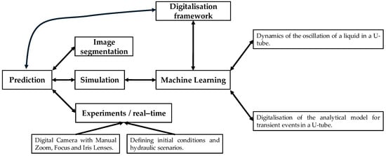
Figure 1.
Proposed digitalisation framework for analysing transient flow in a U-tube.
The steps for implementing the methodology are presented below, where the components of simulation, experiments, and machine learning (ML) are detailed in the following subsections.
2.1. Empirical Models
This section presents the governing equations used for the digitalisation. Equation (1) is a second-order ordinary differential equation that can be used to analyse different physical processes, all of them related to the damped oscillation processes, which in engineering has the following applications: (i) oscillation of a liquid in a U-tube, (ii) an oscillating mass hanging from a spring, (iii) the pendulum equation, (iv) variation in voltage in an electronic circuit, and (v) the gravitational law and motion of satellites.
For each case mentioned above, the and coefficients have their physical meaning for our case of study, the oscillating movement of a liquid in a U-tube, is the space, is the time, is a friction coefficient, is the natural frequency of the movement and is the external forcing.
To study the oscillation of a liquid in a U-tube, the liquid-wall resistance, represented by the α coefficient in Equation (1), plays a vital role in the solution of the equation, considering three types of resistance (no resistance at all, laminar and turbulent). In addition to the resistance, the movement may be subject to external forcing, the function in Equation (1), considered a harmonic function in this research. Table 1 presents the equations for the three cases, their associated parameters, and the type of solution that can be obtained for each (analytical/numerical). The equations are presented in terms of , the meniscus position, as the dependent variable and time (), as the independent variable. The meniscus velocity and acceleration are obtained by applying the first and second derivatives of displacement () over time. The kinetic and potential energy associated with the movement can also be computed at any time.

Table 1.
Differential equations governing the flow of a liquid in a U-tube.
The velocity distribution approximately represents the velocity gradient as [26]:
where the parameter depends on the Reynolds number as stated in Table 1, is the flow mean velocity and is the tube radius.
The analytical and numerical solutions implemented include several features: (a) the forcing function was considered as a sine function with any frequency; (b) over-damped, critically damped and under-damped oscillations [28,29] where implemented for laminar resistance considering all the attributes assigned to the forcing function; (c) for turbulence resistance, for which no analytical solution is available, except for specific points in time (critical, maximum or minimum point of ) a numerical method is required to find the solution, being the 4th order Runge–Kutta method the one implemented.
For all the solutions implemented, the initial conditions for the meniscus position and the meniscus velocity were set as:
2.2. Experimental Stage
The experiment setup (see Figure 2) consists of a U-glass tube with an inner diameter of 14.2 mm and a total length of 1.5 m. A plastic hose is attached at one end of the tube to generate suction and initiate the motion. The analysed fluid is water. If a forcing term is to be simulated, the proper mechanism must be connected to the hose. A video camera is mounted on a tripod 1.6 m away from the board to which the U-tube is attached and levelled so that its optical axis is perpendicular to that plane, so there is no need to rectify the image during the image processing stage. The camera is connected to a PC to save the video and employ a code for image processing. In the upper left corner of Figure 2, a zoom of the setup shows four dots (control points) set 92 mm apart in both the vertical and horizontal directions, used to determine the pixel size for the digital images. A hose connected to a syringe was attached to one end of the U-tube in order to generate an initial pressure difference and thereby induce oscillation of the fluid column. Once the motion commenced, both ends were exposed to atmospheric pressure. As noted previously, the temporal variation in the meniscus position was recorded, from which the velocity and acceleration of the fluid column were derived. The dynamic pressure of the fluid can then be estimated from the calculated velocity.
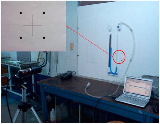
Figure 2.
Experiment setup: U-tube, liquid (in blue), digital camera, PC and control dots to obtain the pixel size of the captured images.
The experiment setup for the phenomenon studied is an arrangement of a U-tube of constant diameter filled with a liquid (water, as reported in the results). Table A1 presents the initial conditions of the experimental measurements, along with their corresponding temperatures during the measurements. The meniscus position is obtained by recording it with a digital camera, generating a video, which is later processed using image processing techniques.
During the experimental measurements, the U-tube was not employed to measure dynamic pressure. Instead, the temporal variation in the meniscus position was recorded, from which the velocity and acceleration of the fluid column were determined by applying the first and second derivatives of with respect to time.
Considering that the experiments were conducted using a glass pipe with an internal diameter of 14.2 mm, a water surface tension of 0.072 N/m, and a contact angle between water and glass ranging from 0° to 30° [30], the Young–Laplace equation yields an average meniscus rise of approximately 3 mm. In this study, this elevation is not considered significant, as it does not noticeably affect the natural oscillation frequency. This was verified by calculating the error between the theoretical and experimental natural oscillation periods, the latter being obtained through spectral analysis of the meniscus position derived from laboratory image processing. The results are presented in Table A2, where it can be observed that the maximum absolute error was 0.010 s, while the maximum relative error did not exceed 0.8%.
Table 2 shows the characteristics of the digital camera (Stringray F-080B/C camera), and Table 3 presents the characteristics of its lenses.
Table 2.
Characteristics of the Stringray F-080B/C digital camera.
Table 3.
Characteristics of the lenses.
2.3. Machine Learning
Machine Learning (ML) can be employed to capture patterns and relationships for the study of transient events in a U-tube. Such algorithms may be applied at various stages of the proposed methodology, ranging from the acquisition and processing of digital images to the training of a model capable of predicting system behaviour based on simulation results. ML is used to indicate the behaviour of transient flow in a U-tube as well as to digitalise the governing equations that describe the system. The software MATLAB (R2024b) has been used for making calculations. In this research, twenty-eight algorithms were employed to select the best one, obtaining that the best results were achieved using the robust linear regression and Squared Exponential Gaussian Process Regression, which are described below.
2.3.1. Robust Linear Regression
This algorithm is similar to a linear regression model, but it uses an iteratively reweighted least squares method to assign weights to observations. The main advantage of this algorithm is that it is less sensitive to outliers compared to the traditional one.
where corresponds to the response, represents each observation, is a coefficient, is an observation on the predictor, is the noise term, and is the number of total predictors.
The estimation of the weighted least-square error is yielded by:
where corresponds to the weights, represents each one of responses, and corresponds to the fitted responses.
2.3.2. Squared Exponential Gaussian Process Regression
The formula represents this probabilistic model:
where corresponds to the response, is a latent variable, are each one of predictors, is a matrix of basis functions, represents a coefficient based on the dataset, is the identity matrix, and is the error variance used by the model.
2.4. Image Segmentation
Employing the digital camera described in Section 2.2, image segmentation was performed to extract digital information and track variations in meniscus position. The methodology used to capture and process the digital images is presented as follows:
- (a)
- Level the tripod and the camera.
- (b)
- Manually focus and set the zoom and the iris opening for the camera.
- (c)
- Before initiating the video of the liquid column in movement, a photo (“stack”) is taken at the control points (see Figure 2). This photograph is used to compute the image’s pixel size in metres. Due to the small distance from the camera to the plane where the U-tube is attached (d ≈ 1.6 m) and given that the captured area to be recorded (the meniscus) will be located at the centre of every image, the radial distortion of the images is negligible. It will not be considered in the image processing calculations. The centre of mass of the circles of the control points is calculated, and the number of digital pixels between two control points is counted (vertically and horizontally) using MATLAB (version 2024b). The centre of mass of the circles in the image with the control points is located. Then, the script counts the number of pixels between the centre of mass of two control points, aligned vertically and horizontally. Finally, the size of a pixel, in metres, is obtained from the linear relationship shown below:where = pixel (m), = distance between control points (m), and = number of pixels between control points.
- (d)
- The camera is configured to save a video at a desired frequency (frames per second or fps), 30 fps in our case, and with a desired spatial resolution (100 pixels, horizontal × 768 pixels, vertical in our case). The video is saved for one of the tube branches, capturing the meniscus movement. It is recommended that the video be started before the meniscus movement begins, so it will be possible to identify the time of motion initiation later.
- (e)
- Once the video is completed, the image processing is initiated by breaking it into individual frames, and each one is processed by capturing the pixel intensity through a complete column of pixels of each frame, giving. Figure 3a shows the first 14 frames of an experimental test for illustrative purposes. The total number of frames varies depending on the video duration and capture frequency. Figure 3b presents the frequency spectrum of one of the laboratory tests, calculated from the experimentally obtained meniscus position data. It shows a dominant peak at the natural oscillation frequency, indicating that the oscillation of a fluid column in a U-tube behaves as a simple harmonic oscillator, analogous to a pendulum. The remaining tests likewise exhibited a dominant peak. From the dominant frequency f0 (corresponding to the natural oscillation of the fluid column) in each test, we calculated the natural oscillation period as T = 1/f0. As a result, a column of “coloured” pixels for each frame (Figure 4a). The contrast of colours between the one obtained for the meniscus (blue) and that for the U-tube background (grey) was enough to process the images adequately. Every frame is analysed using different filters (different colour bands, including red, green, and blue), with the red band yielding the highest contrast (see Figure 4b–d) to identify images with the most significant contrast between the meniscus and the U-tube background. In Figure 4, a shade in the interface corresponds to the meniscus reflection over the tube material.
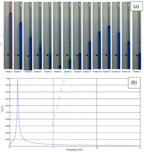 Figure 3. Characterisation of oscillations: (a) number of frames from an experimental test; and (b) frequency spectrum of an experimental measurement.
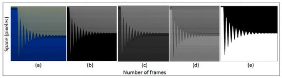 Figure 4. RGB image chosen from all frames, at different colour bands, where the meniscus was identified: (a) image with all frames; (b) red band; (c) green band; (d) blue band; and (e) the resulting binary image.
- (a)
- The filtered image is then converted into a binary image by setting a limit pixel intensity. To define this limit, it is assumed that the histogram of the binary image is bimodal, a valid assumption given the high contrast between the liquid and the tube background, as shown clearly in Figure 4a. The definition of the limit pixel intensity is obtained by following the methodology suggested by Ridler-Calvard [31,32]. The binary image is shown in Figure 4e, where the white “pixels” correspond to the liquid. This information is saved in a file in a matrix form of “0” and “1,” with each column containing the binary information of a column of pixels of each frame.
- (b)
- With the binary image, the location of the meniscus is the next step. To do this, the “binary matrix (of order n pixels per row x m frames)” is used to locate the position (in terms of row number of this matrix) of the first “0” pixel at every column of the matrix. This position is found by sweeping the matrix from row 1 to row n for every column. This search is performed for every binary image in the video, each corresponding to a specific time (each video frame is assigned a time).
- (c)
- From the time series of the meniscus positions, the time of the initiation of meniscus motion (t0) is determined by the following criteria: checking the time corresponding to a series of 5 consecutive frames that do not show any changes in the meniscus position (5 was set for our case after several trials).
- (d)
- To locate the meniscus position concerning the no-motion position (equilibrium position with the liquid at rest, the reference level in the governing equations), the series of meniscus positions is recalculated by obtaining the average position. The previously calculated pixel size converts this new series into units of length.
- (e)
- Once the meniscus position is obtained, its velocity and acceleration are computed by a numerical differentiation of the meniscus position time series, each corresponding to a binary image with a time “coordinate” assigned. The meniscus velocity and acceleration are computed as:
3. Results
A set of 27 tests, with different lengths of liquid column (63.14 cm < < 98.50 cm) and initial meniscus position (1.97 cm < < 24.40 cm), were performed. At the beginning of each test, the liquid temperature was measured, and its physical properties were obtained from fluid mechanics textbooks [33,34]. The liquid column length was determined indirectly by measuring the volume of liquid poured into the tube and assuming a constant inner diameter of the tube. The simulation provides the maximum Reynolds number computed as shown by Equations (6) and (7). For the 27 tests, a maximum value of 21086 and a minimum value of 1827 were obtained, indicating a range of values that suggests the experiments were conducted under both laminar-turbulent and laminar regime conditions in some cases.
Two cases for the error analysis are presented in this study: the first corresponds to the experiment oscillation period in comparison with the natural period of oscillation of our system, and the second corresponds to the meniscus position ().
The theoretical natural period of oscillation, according to the Newtonian theory, for the meniscus oscillation in a U-Tube is:
This period is modified when the liquid’s viscosity is considered for such oscillations under turbulent friction. According to Reference [26], this period is calculated as:
where represents the length of the liquid, is a velocity correction factor that depends on the Reynolds number (see Table 1), is the kinematic viscosity, and is the internal radius of the tube.
The experimental value of the oscillation period was obtained from the frequency spectrum calculated from the measured time series (obtained from the processed digital images) of the meniscus position (). For all 27 tests, the frequency analysis showed a highly dominated one-peak spectrum, and the maximum error found between [26] and the experimental value was 0.6% except for tests 25 and 26, which reached 1.1%. As shown later, the model fits the experimental tests better than the Newtonian approach [26], so the period given by Equation (9) will be used for error calculations.
The simulation performed on the measured data in comparison to the analytical/numerical resolutions closely follows the methodology from [35,36], which suggests a methodology to separate the systematic error (RMSEs) from the nonsystematic error (RMSEu) and computes the Index of an agreement to measure the degree to which a model prediction is error-free. It is necessary to calculate the following parameters to evalute the potential precision of a model: mean value of the predictions , the mean value of the observations , the standard deviation of the predictions and of the observations , the intercept (a) and the slope (b) of the least square regression , the mean absolute error (MAE), the mean square error (MSE), the root mean square error (RMSE), the systematic mean square error (MSEs), the square root of MSEs (RMSEs), the nonsystematic mean square error (MSEu), the square root of MSEu (RMSEu), the coefficient of determination () and the index of agreement (). The complete set of statistical parameters used by this methodology is listed in Table 4. Given that all data from measurements have an intrinsic error associated with their measuring method, it emphasises the importance of estimating the fraction of the RMSEs that correspond to the RMSE and the fraction of the RMSEu that corresponds to the RMSE. Additionally, it is of utmost importance to consider the values of the or associated with high errors being hidden when the and values are high. To overcome this interpretation, the index of agreement () is recommended, which measures the degree to which the observed (measured) variable is estimated by the simulated one (0 value means no agreement at all and a value of 1 represents a perfect agreement). Given this index’s dimensionless property, it tends to complement the information provided by the RMSE, RMSEs and RMSEu parameters. The RMSEu parameter can be interpreted as a measurement of the potential precision of the model; that is, it is possible that with minor changes in the model structure, the RMSE value can be reduced significantly.
Table 4.
Statistical parameters.
As a first step for validating the solutions, the index of agreement was calculated for all 27 experiments. Values between 0.95 and 0.99 were obtained, indicating good agreement between the analytical/numerical resolutions.
As a second step in the validation, the methodology was used to analyse the MSEs and MSEu parameters for the 27 experiments studying the effect of the Newtonian and the selected [26] friction models. For each experiment, three different scenarios were considered, which are described below:
- (a)
- In the first scenario, the Newtonian model is applied to the solution in turbulent and laminar regimes.
- (b)
- In the second scenario, Ogawa’s friction model is used for laminar flow, and Newtonian is used for turbulent flow.
- (c)
- In the third scenario, Ogawa’s friction model is used for laminar and Turbulent flow. Notice that this model was initially developed for both regimes.
After running the experiments and their corresponding analytical/numerical resolutions, the RMSEu parameter was computed for all the experiments and the three scenarios mentioned earlier. The results of these computations are presented in Figure 5, which clearly shows a better behaviour of Ogawa’s friction model. For all cases, there is a general tendency for the RMSEu to increase with an increment in the Reynolds number. The RMSEu can be interpreted as a measure of the potential accuracy of a model. In this context, the increase in RMSEu with higher Reynolds numbers is attributed to the fact that the friction relationships used in the theoretical (Newtonian) model—against which the experimental data are compared—are less accurate for flows with very high Reynolds numbers. At such regimes, friction may become unstable, the curvature of the pipe can introduce additional frictional effects, and fluid–structure interaction may play a significant role.
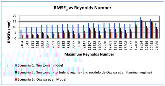
Figure 5.
RMSEu versus Reynolds number for all 27 experiments.
A different behaviour was observed for the RMSEs (see Figure 6), which now, for large Reynolds numbers (), the Ogawa et al. model behaves poorly while for small Reynolds numbers behaves much better than for the other two scenarios. Following the methodology from [35,36]. This behaviour can be associated with an improper parameterisation of the model, so adjusting certain parameters can improve the solution. In our case, Ogawa’s model is characterised by a parameter related to the velocity distribution, defined in Equation (2), the parameter. This parameter depends on an empirical coefficient (see Table 1). A fourth scenario was run to improve the solution by setting the α coefficient to a new value of 29. Modifying this coefficient is justified by giving the range of validity set for the original experiments by Reference [26], which was for a maximum Reynolds number of 6600. The new value of = 29 was obtained by looking for the best fitting option, and for the experiments with . Figure 7 shows the best results obtained for Reynold numbers that are more significant than 16,000.
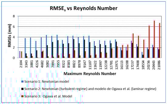
Figure 6.
RMSEs versus Reynolds number for all 27 experiments.
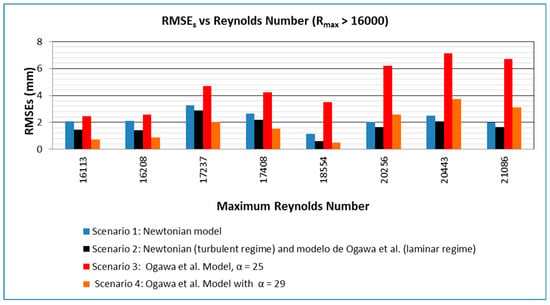
Figure 7.
RMSEs versus Reynolds number ().
The systematic error highly depends on the degree of resolution, the calibration level of the measuring instruments and the measuring procedures. However, this error also depends on the accumulation of rounding errors in the numerical model, particularly when estimating a quantity without direct measurement. In this case, assuming that 100% of the RMSEs are due to the measuring technique (video measurements), and considering the range , the mean error was computed to be of the order of 2.2 mm or of the order of 3 pixels, result which is in accordance with the one obtained for the error in the oscillation period. This is an encouraging result for the video measuring technique.
Two cases of extreme values of the Reynolds number (test 14 and test 8) are reported to illustrate the behaviour of all parameters suggested. The experimental conditions, as shown in Table 5, and the list of statistics in Table 6; Table 7, respectively.
Table 5.
Experiment conditions for Tests 14 and 8.
Table 6.
Statistical parameters for test 14.
Table 7.
Statistical parameters for test 8.
Test 8 (Table 6) for , the best statistic parameters are obtained for the original Ogawa ed al. model ( = 25). The index of agreement does not show significant differences between the scenarios, but the parameter does show differences, with the Ogawa et al. model showing the highest value. All the parameters confirm that the Ogawa et al. model is the best.
For high Reynolds numbers (, e.g., Test No. 8 (see Table 7), the statistical parameters exhibit the same behaviour as in the experiments with low Reynolds numbers, albeit with a more significant difference in the statistical parameter values in favour of the improved model by Ogawa’s friction model ( = 29). It is also noteworthy that, in this case, the index of agreement and the parameter show better values than those obtained using the original Ogawa’s friction model ( = 25).
Figure 8 shows a comparison of the meniscus position obtained from the measurements with that computed by the simulation for the three scenarios mentioned earlier, for experiments 14, where the yellow strips indicate the turbulent flow regime . It is clear from these figures that the Newtonian friction model behaves poorly with respect to the measurements. The computed and measured meniscus velocity for the three scenarios is presented in Figure 9 for experiment 14, and the meniscus accelerations are shown in Figure 10 for experiment 14. Notice that the measured velocity and accelerations show oscillations due to the mathematical procedure used to numerically compute the first and second derivatives from the meniscus position time series.
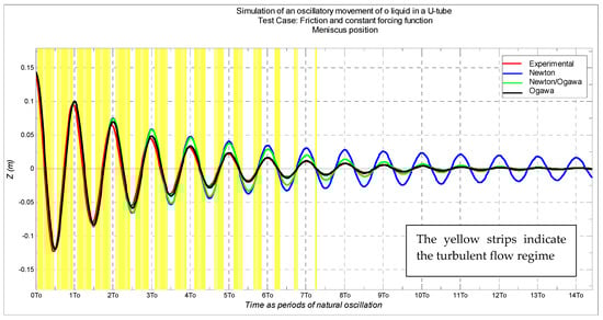
Figure 8.
Variation in the meniscus position in time (as a function of the natural period of oscillation) for measurements and the three scenarios related to the friction model for test 14.
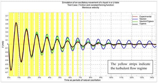
Figure 9.
Variation in the meniscus velocity in time (as a function of the natural period of oscillation) for measurements and the three scenarios related to the friction model for experiment 14.
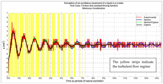
Figure 10.
Variation in the meniscus acceleration in time (as a function of the natural period of oscillation) for measurements and the three scenarios related to the friction model for experiment 14.
Machine learning (ML) techniques were employed to demonstrate their applicability in studying the dynamics of oscillations in a U-tube through the digitalisation of the differential equations described in Section 2.1. In this study, the model was trained using a dataset comprising 27 measurements. To mitigate overfitting, five-fold cross-validation was employed, and 30% of the data was reserved for testing purposes. The length of the liquid () and the initial position of the meniscus were employed as predictors using ML. Two responses were evaluated in this model using the natural period of oscillation () and the minimum position reached by the meniscus (). Figure 11 presents the relationships between the two predictors and their corresponding responses.
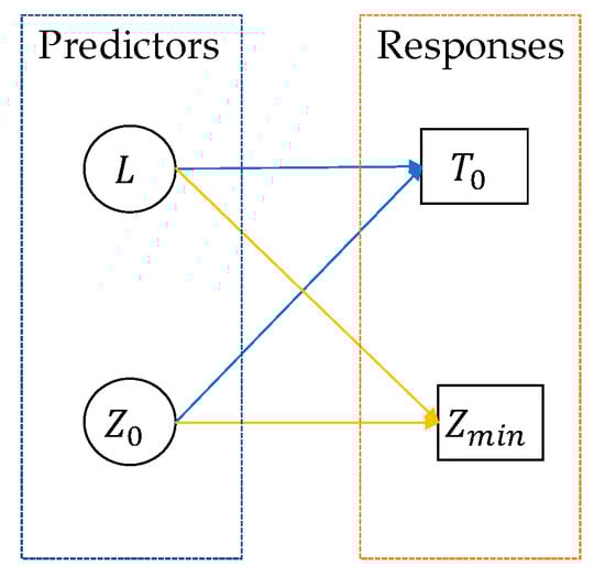
Figure 11.
Relationships between predictors and responses for applying ML.
Twenty-eight machine learning models were employed to train the model described previously, as defined by the equations in Section 2.1. Table 8 presents the results of the statistical metrics (R2 and RMSE) for the ML models. The findings indicate that ML models are well-suited for capturing the dynamics of a transient event in a U-tube. In particular, the most favourable statistical performance for the minimum meniscus position and the natural oscillation period was obtained using the robust linear method and the Squared Exponential Gaussian Process Regression, respectively. The selection of these models was informed by statistical measures obtained from both the validation and testing stages. The best-performing ML models, in which, in all cases, the R2 values for both the validation and testing stages are above 0.997, while the corresponding RMSE values are notably low.
Table 8.
Summary of the statistical measures of ML models.
4. Discussion
The developed methodology aimed to improve the understanding of the physical processes involved in damped oscillations of a liquid in a U-tube by digitalising all components. One advantage of the developed methodology is that it includes a step to process the digital images captured from the physical experiments using state-of-the-art techniques to process digital photos [37,38,39,40,41]. In addition, image segmentation can be performed using deep learning techniques on both visual and numerical data to investigate the dynamics within a U-tube.
By applying the methodology from [35,36], it was possible to separate the MSEs from the MSEu, and an estimate for the error associated with the experimental technique was determined. The error analysis was performed for the friction model by considering four scenarios. The study revealed that Ogawa’s friction formula is the most effective model. The results show a systematic error of 2.2 mm for the model [26] about the measurements. Additionally, a minor error (as significant as 1.1%) was observed in the period of oscillation for all 27 test cases. The video camera measurement technique proved suitable for this type of experiment.
For the tests with it was necessary to improve the selected model [26] setting a new value for the α parameter associated with the assumed velocity distribution led to a smaller value for RMSEs. Modification of the α parameter was supported by the fact that the original model was tested for .
Similar results were found by Olan Thon, B. (2014) [9], who concluded that the model by Ogawa et al. is more effective than other steady friction relationships in damping oscillations in a U-tube. However, it does not yield satisfactory results for high Reynolds numbers, likely because the model was developed with low Reynolds numbers in mind. The Ogawa’s friction model exhibits the same velocity dependence as the laminar friction factor, making it highly effective for low Reynolds numbers but less so for high Reynolds numbers.
Using digital images as a measuring technique for these experiments was proven suitable, given the minor errors obtained for the pixel size.
The machine learning models were successfully applied to investigate the dynamics of a U-tube, with statistical measures indicating reliable performance. This is especially significant, as ML has the potential to support predictive capabilities, thereby playing a crucial role in implementing a digitalisation of mathematical models. This virtual representation enables real-time monitoring, scenario testing, and optimisation without disrupting the physical system.
5. Conclusions
This study presented the digitalization process for studying transient events in a U-tube, comprising the following steps: (i) a simulation process, in which the numerical solution of the governing equations for damped oscillatory phenomena was developed and validated for the specific case of liquid oscillation in a U-tube; (ii) an image segmentation process for tracking the meniscus position; and (iii) a layer containing detailed information about the hydraulic installation. The proposed methodology was supported by an experimental facility measuring 1.5 m in length.
The implementation of machine learning techniques proved to be an effective strategy for digitalising the complex governing equations that describe the hydraulic behaviour of a transient event in a U-tube. Moreover, machine learning techniques can be applied to enable rapid decision-making, as there is no need to solve complex equations in real-time. Consequently, predictive analyses can be readily conducted using this tool. Statistical measures, such as the coefficient of determination and the root mean square error, confirmed its applicability.
Author Contributions
Conceptualization, A.A.-P. and E.A.M.-P.; methodology, E.A.M.-P.; formal analysis, E.A.M.-P.; software, E.A.M.-P., M.S., V.S.F.-M. and O.E.C.-H.; writing—original draft preparation, E.A.M.-P., A.A.-P., M.S. and O.E.C.-H.; writing—review and editing, V.S.F.-M. All authors have read and agreed to the published version of the manuscript.
Funding
This research received no external funding.
Institutional Review Board Statement
Not applicable.
Informed Consent Statement
Not applicable.
Data Availability Statement
The original contributions presented in this study are included in the article. Further inquiries can be directed to the corresponding author(s).
Acknowledgments
The authors wish to acknowledge the support provided by the School of Mines at the Universidad Nacional de Colombia, Medellín Campus, for the financial support to the first author (E.A.M.-P.).
Conflicts of Interest
The authors declare no conflicts of interest.
Abbreviations
The following abbreviations are used in this manuscript:
| = | Pipe diameter (m); |
| = | Distance between control points (m); |
| = | Darcy-Weisbach friction coefficient (−); |
| = | Dominant frequency (Hz); |
| = | External forcing function (m); |
| = | Gravitational acceleration (m/s2); |
| = | Matrix of basis functions; |
| = | Identity matrix; |
| = | Observation (−); |
| = | Velocity correction factor (−); |
| = | Length of the liquid column (m); |
| = | Number of pixels between control point (−); |
| = | Pixel (m); |
| = | Number of total predictors (−); |
| = | Tube radius (m); |
| = | Reynolds number (−); |
| = | Natural oscillation (s); |
| = | Time (s); |
| = | Meniscus velocity (m/s); |
| = | Weighted least-square error (−); |
| = | Distance (m); |
| / = | Predictor (m); |
| = | Response (s or m); |
| = | Fitted responses (s or m); |
| = | Meniscus position (m); |
| = | Pressure difference (Pa); |
| = | Liquid kinematic viscosity (m2/s); |
| = | Natural frequency (Hz); |
| = | Forcing frequency (Hz); |
| = | Noise term; |
| = | Friction coefficient (−); |
| = | Natural frequency coefficient (−)/Coefficient of a machine learning model (−); |
| = | Liquid density (kg/m3); |
| = | Error variance; |
| 0 = | Initial condition. |
Appendix A
Table A1.
Dataset of initial conditions of experimental measurements.
Table A1.
Dataset of initial conditions of experimental measurements.
| Run No. | ||||||
|---|---|---|---|---|---|---|
| (°C) | (kg/m3) | (m2/s) | (mm) | (cm) | (cm) | |
| 1 | 26.20 | 997.10 | 8.74 × 10⁻⁷ | 14.2 | 63.14 | 22.77 |
| 2 | 26.80 | 8.63 × 10⁻⁷ | 18.96 | |||
| 3 | 27.30 | 8.54 × 10⁻⁷ | 9.58 | |||
| 4 | 2.40 | |||||
| 5 | 4.80 | |||||
| 6 | −19.17 | |||||
| 7 | −10.45 | |||||
| 8 | 72.62 | 24.97 | ||||
| 9 | 10.13 | |||||
| 10 | 15.81 | |||||
| 11 | −24.61 | |||||
| 12 | −15.55 | |||||
| 13 | 27.60 | 8.48 × 10⁻⁷ | 83.98 | 20.92 | ||
| 14 | 27.50 | 8.50 × 10⁻⁷ | 15.16 | |||
| 15 | 27.30 | 8.54 × 10⁻⁷ | 10.25 | |||
| 16 | 4.28 | |||||
| 17 | −24.33 | |||||
| 18 | −16.11 | |||||
| 19 | 21.08 | |||||
| 20 | 15.57 | |||||
| 21 | 10.28 | |||||
| 22 | 4.66 | |||||
| 23 | 98.50 | 12.08 | ||||
| 24 | 6.92 | |||||
| 25 | −15.48 | |||||
| 26 | 12.54 | |||||
| 27 | 7.11 |
Note: = temperature, = water density, = water kinematic viscosity, = internal pipe diameter, = length, and = initial position of the meniscus.
Table A2.
Computation of absolute and relative error of experimental measurements.
Table A2.
Computation of absolute and relative error of experimental measurements.
| Run No. | (cm) | (s) | Absolute Error (s) | Relative Error (%) | |
|---|---|---|---|---|---|
| 1 | 63.14 | 1.127 | 1.133 | 0.006 | 0.545 |
| 2 | 1.136 | 0.008 | 0.742 | ||
| 3 | 1.136 | 0.008 | 0.742 | ||
| 4 | 1.133 | 0.006 | 0.545 | ||
| 5 | 1.136 | 0.008 | 0.742 | ||
| 6 | 1.136 | 0.008 | 0.742 | ||
| 7 | 1.136 | 0.008 | 0.742 | ||
| 8 | 72.62 | 1.21 | 1.217 | 0.008 | 0.653 |
| 9 | 1.217 | 0.008 | 0.653 | ||
| 10 | 1.217 | 0.008 | 0.653 | ||
| 11 | 1.214 | 0.006 | 0.456 | ||
| 12 | 1.217 | 0.008 | 0.653 | ||
| 13 | 83.98 | 1.3 | 1.310 | 0.010 | 0.794 |
| 14 | 1.310 | 0.010 | 0.794 | ||
| 15 | 1.310 | 0.010 | 0.794 | ||
| 16 | 1.310 | 0.010 | 0.794 | ||
| 17 | 1.310 | 0.010 | 0.794 | ||
| 18 | 1.310 | 0.010 | 0.794 | ||
| 19 | 1.308 | 0.008 | 0.596 | ||
| 20 | 1.308 | 0.008 | 0.596 | ||
| 21 | 1.308 | 0.008 | 0.596 | ||
| 22 | 1.308 | 0.008 | 0.596 | ||
| 23 | 98.5 | 1.41 | 1.417 | 0.009 | 0.626 |
| 24 | 1.417 | 0.009 | 0.626 | ||
| 25 | 1.417 | 0.009 | 0.626 | ||
| 26 | 1.417 | 0.009 | 0.626 | ||
| 27 | 1.417 | 0.009 | 0.626 |
References
- Yang, B.; Deng, J.; Yuan, W.; Wang, Z. Investigation on Continuous Pressure Wave in a Periodic Transient Flow Using a Three-Dimensional CFD Model. J. Hydraul. Res. 2020, 58, 172–181. [Google Scholar] [CrossRef]
- Mousavifard, M.; Poursmaeili, F.; Shamloo, H. Development of Backward Transient Analysis in Visco-Elastic Pressurized Pipes. J. Hydraul. Res. 2022, 60, 423–433. [Google Scholar] [CrossRef]
- Zeidan, M.; Németh, M.; Abhijith, G.R.; Wéber, R.; Ostfeld, A. Transient Flow Dynamics in Tesla Valve Configurations: Insights from Computational Fluid Dynamics Simulations. Water 2024, 16, 3492. [Google Scholar] [CrossRef]
- Wang, Q.; Hu, J.; Song, M.; Shen, H.; Zhou, Y.; Li, D.; Xie, F. Study on the Transient Flow Characteristics of a Hump Water Pipeline Based on the Random Distribution of Bubbles. Water 2023, 15, 3831. [Google Scholar] [CrossRef]
- Brown, C.S.; Kolo, I.; Banks, D.; Falcone, G. Comparison of the Thermal and Hydraulic Performance of Single U-Tube, Double U-Tube and Coaxial Medium-to-Deep Borehole Heat Exchangers. Geothermics 2024, 117, 102888. [Google Scholar] [CrossRef]
- Ligus, G.; Wasilewska, B. Maldistribution of a Thermal Fluid along the U-Tube with a Different Bending Radius—CFD and PIV Investigation. Energies 2023, 16, 5716. [Google Scholar] [CrossRef]
- Munguía, H.; Franco, R.; Barba, L. Liquid Oscillations in a U-Tube. Phys. Educ. 2018, 53, 015005. [Google Scholar] [CrossRef]
- Mungan, C.; Sheldon-Coulson, G. Liquid Oscillating in a U-Tube of Variable Cross Section. Eur. J. Phys. 2021, 42, 025008. [Google Scholar] [CrossRef]
- Olav Thon, B. Friction Models for Oscillating Flow in a U-Tube. Master’s Dissertation, Norwegian University of Science and Technology, Nanjing, China, 2014. [Google Scholar]
- Miller, J.; Werth, D. Recirculating Flow in Oscillatory U-Tubes. J. Hydraul. Eng. 2005, 131, 397–403. [Google Scholar] [CrossRef]
- Kannaiyan, A.; Karuppa, T.; Sarno, L.; Urbanowicz, K.; Martino, R. A Generalized Mathematical Model for the Damped Free Motion of a Liquid Column in a Vertical U-Tube. Phys. Fluids 2024, 36, 103626. [Google Scholar] [CrossRef]
- Liang, Y.; Xi, G.; Sun, Z. Numerical Study of the Damped Oscillation of Liquid Column in U-Tube with Particle Method. J. Fluids Eng. Trans. ASME 2013, 135, 061202. [Google Scholar] [CrossRef]
- Zechman, B.E.; Ehsan, S.M.; Lu, X.; Jason, W. Digital Twins for Water Distribution Systems. J. Water Resour. Plan. Manag. 2023, 149, 02523001. [Google Scholar] [CrossRef]
- Ramos, H.M.; Kuriqi, A.; Coronado-Hernández, O.E.; López-Jiménez, P.A.; Pérez-Sánchez, M. Are Digital Twins Improving Urban-Water Systems Efficiency and Sustainable Development Goals? Urban. Water J. 2023, 21, 1164–1175. [Google Scholar] [CrossRef]
- Paternina-Verona, D.A.; Coronado-Hernández, O.E.; Fuertes-Miquel, V.S.; Saba, M.; Ramos, H.M. Digital Twin Based on CFD Modelling for Analysis of Two-Phase Flows During Pipeline Filling–Emptying Procedures. Applied Sciences 2025, 15, 2643. [Google Scholar] [CrossRef]
- Kim, Y.; Oh, J.; Bartos, M. Stormwater Digital Twin with Online Quality Control Detects Urban Flood Hazards under Uncertainty. Sustain. Cities Soc. 2025, 118, 105982. [Google Scholar] [CrossRef]
- Conejos Fuertes, P.; Martínez Alzamora, F.; Hervás Carot, M.; Alonso Campos, J.C. Building and Exploiting a Digital Twin for the Management of Drinking Water Distribution Networks. Urban. Water J. 2020, 17, 704–713. [Google Scholar] [CrossRef]
- Bartos, M.; Kerkez, B. Pipedream: An Interactive Digital Twin Model for Natural and Urban Drainage Systems. Environ. Model. Softw. 2021, 144, 105120. [Google Scholar] [CrossRef]
- Bonilla, C.; Brentan, B.; Montalvo, I.; Ayala-Cabrera, D.; Wu, J.; Bonilla, C.; Brentan, B.; Montalvo, I.; Ayala-Cabrera, D.; Izquierdo, J. Digitalization of Water Distribution Systems in Small Cities, a Tool for Verification and Hydraulic Analysis: A Case Study of Pamplona, Colombia. Water 2023, 15, 3824. [Google Scholar] [CrossRef]
- Bernard, M. Using Digital Twins to Improve Pumping and Distribution System Operations. J. AWWA 2024, 116, 6–15. [Google Scholar] [CrossRef]
- Ramos, H.M.; Morani, M.C.; Carravetta, A.; Fecarrotta, O.; Adeyeye, K.; López-Jiménez, P.A.; Pérez-Sánchez, M. New Challenges towards Smart Systems’ Efficiency by Digital Twin in Water Distribution Networks. Water 2022, 14, 1304. [Google Scholar] [CrossRef]
- Besharat, M.; Rabbani, A.; Yang, X.; Martinez, J.S.; Moran, V.; Evans, B.; Ramos, H. Data-Driven Predictive Analysis and Visualisation of Air–Water Dynamics in an Air Vessel. J. Hydroinform. 2025, 27, 787–804. [Google Scholar] [CrossRef]
- Ronneberger, O.; Fischer, P.; Brox, T. U-Net: Convolutional Networks for Biomedical Image Segmentation Bt- Medical Image Computing and Computer-Assisted Intervention. In Proceedings of the MICCAI 2015, Munich, Germany, 5–9 October 2015. [Google Scholar]
- Hubert, C.; Xinqian, L. Acoustic Doppler Velocimetry in Transient Free-Surface Flows: Field and Laboratory Experience with Bores and Surges. J. Hydraul. Eng. 2024, 150, 04024034. [Google Scholar] [CrossRef]
- Besharat, M.; Coronado-Hernández, O.E.; Fuertes-Miquel, V.S.; Viseu, M.T.; Ramos, H.M. Backflow Air and Pressure Analysis in Emptying a Pipeline Containing an Entrapped Air Pocket. Urban. Water J. 2018, 15, 769–779. [Google Scholar] [CrossRef]
- Ogawa, A.; Tokiwa, S.; Mutou, M.; Mogi, K.; Sugawara, T.; Watanabe, M.; Satou, K.; Kikawada, T.; Shishido, K.; Matumoto, N. Damped Oscillation of Liquid Column in Vertical U-Tube for Newtonian and Non-Newtonian Liquids. J. Therm. Sci. 2007, 16, 289–300. [Google Scholar] [CrossRef]
- Bacelar, M.D.; Ferreira, H.C.M.G.; Alassar, R.S.; Lopes, A.B. Hagen-Poiseuille Flow in a Quarter-Elliptic Tube. Fluids 2023, 8, 247. [Google Scholar] [CrossRef]
- Griffiths, D.V.; Smith, I.M. Numerical Methods for Engineers; Chapman and Hall/CRC: Boca Raton, FL, USA, 2006; ISBN 0429149212. [Google Scholar]
- Hoffman, J.D.; Frankel, S. Numerical Methods for Engineers and Scientists; CRC press: Boca Raton, FL, USA, 2018; ISBN 1482270609. [Google Scholar]
- Iglauer, S.; Salamah, A.; Sarmadivaleh, M.; Liu, K.; Phan, C. Contamination of Silica Surfaces: Impact on Water–CO2–Quartz and Glass Contact Angle Measurements. Int. J. Greenh. Gas Control. 2014, 22, 325–328. [Google Scholar] [CrossRef]
- Hrytsyk, V.; Borkivskyi, A.; Oliinyk, T. Achieving the Best Symmetry by Finding the Optimal Clustering Filters for Specific Lighting Conditions. Symmetry 2024, 16, 1247. [Google Scholar] [CrossRef]
- Xue, J.-H.; Zhang, Y.-J. Ridler and Calvard’s, Kittler and Illingworth’s and Otsu’s Methods for Image Thresholding. Pattern Recognit. Lett. 2012, 33, 793–797. [Google Scholar] [CrossRef]
- Potter, M.C.; Wiggert, D.C.; Ramadan, B.H. Mechanics of Fluids, 5th ed.; Cengage Learning: Boston, MA, USA, 2001; ISBN 978-1305635173. [Google Scholar]
- Streeter, V.L.; Wylie, E.B. Fluid Mechanics, 7th ed.; McGraw-Hill Higher Education: Reno, NV, USA, 1979; ISBN 13:9780070622326. [Google Scholar]
- Willmott, C.J.; Ackleson, S.G.; Davis, R.E.; Feddema, J.J.; Klink, K.M.; Legates, D.R.; O’Donnell, J.; Rowe, C.M. Statistics for the Evaluation and Comparison of Models. J. Geophys. Res. Ocean. 1985, 90, 8995–9005. [Google Scholar] [CrossRef]
- Willmott, C.J. Some Comments on the Evaluation of Model Performance. Bull. Am. Meteorol. Soc. 1982, 63, 1309–1313. [Google Scholar] [CrossRef]
- Khorchani, M.; Blanpain, O. Free Surface Measurement of Flow over Side Weirs Using the Video Monitoring Concept. Flow Meas. Instrum. 2004, 15, 111–117. [Google Scholar] [CrossRef]
- Erikson, L.H.; Hanson, H. A Method to Extract Wave Tank Data Using Video Imagery and Its Comparison to Conventional Data Collection Techniques. Comput. Geosci. 2005, 31, 371–384. [Google Scholar] [CrossRef]
- Shilton, A.; Bailey, D. Drouge Tracking by Image Processing for the Study of Laboratory Scale Pond Hydraulics. Flow Meas. Instrum. 2006, 17, 69–74. [Google Scholar] [CrossRef]
- Kuo, C.A.; Hwung, H.H.; Chien, C.H. Using Time-Stack Overlooking Images to Separate Incident and Reflected Waves in Wave Flume. Wave Motion 2009, 46, 189–199. [Google Scholar] [CrossRef]
- Mayor, T.S.; Pinto, A.M.F.R.; Campos, J.B.L.M. An Image Analysis Technique for the Study of Gas–Liquid Slug Flow along Vertical Pipes—Associated Uncertainty. Flow Meas. Instrum. 2007, 18, 139–147. [Google Scholar] [CrossRef]


Disclaimer/Publisher’s Note: The statements, opinions and data contained in all publications are solely those of the individual author(s) and contributor(s) and not of MDPI and/or the editor(s). MDPI and/or the editor(s) disclaim responsibility for any injury to people or property resulting from any ideas, methods, instructions or products referred to in the content. |
© 2025 by the authors. Licensee MDPI, Basel, Switzerland. This article is an open access article distributed under the terms and conditions of the Creative Commons Attribution (CC BY) license (https://creativecommons.org/licenses/by/4.0/).