Article

Numerical Study of Gas Dynamics and Condensate Removal in Energy-Efficient Recirculation Modes in Train Cabins

1
Department of Theoretical and Applied Mechanics, Agribusiness Faculty, Don State Technical University, Gagarin, 1, 344003 Rostov-on-Don, Russia
2
Department of Transport Systems, Faculty of Roads and Transport Systems, Don State Technical University, Gagarin, 1, 344003 Rostov-on-Don, Russia
3
Department of Life Safety and Environmental Protection, Faculty of Life Safety and Environmental Engineering, Don State Technical University, Gagarin, 1, 344003 Rostov-on-Don, Russia
4
Department of Transport Engineering, Faculty of Engineering Technology, Don State Technical University, Gagarin, 1, 344003 Rostov-on-Don, Russia
*
Author to whom correspondence should be addressed.
Fluids 2025, 10(8), 197; https://doi.org/10.3390/fluids10080197
Submission received: 8 May 2025 / Revised: 23 July 2025 / Accepted: 26 July 2025 / Published: 29 July 2025

Abstract

Maintaining the required relative humidity values in the vehicle cabin is an important HVAC task, along with considerations related to the temperature, velocity, air pressure and noise. Deviation from the optimal values worsens the psycho-physiological state of the driver and affects the energy efficiency of the train. In this study, a model of liquid film formation on and removal from various cabin surfaces was constructed using the fundamental Navier–Stokes hydrodynamic equations. A special transport model based on the liquid vapor diffusion equation was used to simulate the air environment inside the cabin. The evaporation and condensation of surface films were simulated using the Euler film model, which directly considers liquid–gas and gas–liquid transitions. Numerical results were obtained using the RANS equations and a turbulence model by means of the finite volume method in Ansys CFD. Conjugate fields of temperature, velocity and moisture concentration were constructed for various time intervals, and the dependence values for the film thicknesses on various surfaces relative to time were determined. The verification was conducted in comparison with the experimental data, based on the protocol for measuring the microclimate indicators in workplaces, as applied to the train cabin: the average ranges encompassed temperature changes from 11% to 18%, and relative humidity ranges from 16% to 26%. Comparison with the results of other studies, without considering the phase transition and condensation, shows that, for the warm mode, the average air temperature in the cabin with condensation is 12.5% lower than without condensation, which is related to the process of liquid evaporation from the heated walls. The difference in temperature values for the model with and without condensation ranged from −12.5% to +4.9%. We demonstrate that, with an effective mode of removing condensate film from the window surface, including recirculation modes, the energy consumption of the climate control system improves significantly, but this requires a more accurate consideration of thermodynamic parameters and relative humidity. Thus, considering the moisture condensation model reveals that this variable can significantly affect other parameters of the microclimate in cabins: in particular, the temperature. This means that it should be considered in the numerical modeling, along with the basic heat transfer equations.

1. Introduction

Maintaining the required microclimate parameters in the driver’s cabin is an important task in ensuring comfortable and safe working conditions. The extensive length of Russian railways, which range from north to south and from west to east [1,2] with a large difference in climatic conditions, significantly complicates the work related to the microclimate that needs to be undertaken in order to maintain stable air values.
The key parameters of the microclimate (HVAC [3,4,5,6]) include the characteristics of temperature, air mass velocity, pressure, air humidity and noise. Modern regulatory documents in the field of HVAC [7,8,9,10] provide the required ranges of all relevant parameters but do not touch on the methodologies for developing and modeling microclimate systems and managing them.
The basic methods for constructing dependencies of the air flow, air supply temperature and average speed relative to the temperature characteristics of air inside the cabin include an approach based on energy balance equations. In this approach, the equality of the heat flows in the incoming and outgoing air and the heat exchange through the wall is taken as a given. This method is quite approximate, since it does not consider the significant gradients of temperature and velocity field distribution along the height and width of the cabin. In addition, this approach is associated with the fundamental equation of heat exchange (calculation of the coefficient of convective heat transfer α through the wall into and out of the cabin and into the surrounding air) based on the Nusselt similarity criterion N u = α L / λ , where λ is the thermal conductivity coefficient, in this case, of air, and L is a certain linear measurement associated with the heat-exchange surface [11,12,13]. For the driver’s cabin, the width, length or diagonal of the wall can be used as the linear measurement L. The numerical values of the Nusselt number and the associated heat transfer coefficient are found using the Grashof (Gr) and Prandtl (Pr) criteria [11,12,14,15]. The dimensionless Grashof and Prandtl quantities, in turn, depend on the gas parameters, temperature, characteristic dimensions, and flow speed, as well as on the surface properties. Thus, in a previous study [16], heat exchange in the cabin of the mainline passenger electric locomotive EP20 “Olimp” was investigated; an analysis of the values of heat transfer coefficients was carried out based on formulas applied as determined by the Nusselt criterion and on the solution of complete hydrodynamic equations, and significant discrepancies were indicated in the areas of the gradients of velocity and temperature fields.
Modern trends in the field of computing power development have caused numerical methods of hydrodynamics to be actively implemented [17,18,19]. For heat-exchange problems, the most popular is the volume element method [20] using averaged Navier–Stokes equations in association with the Reynolds method [21,22,23] and turbulence models (RANS). This approach, based on computer fluid dynamics (CFD) [24,25,26], allows for fundamental equations of hydrodynamics and energy to be solved in an explicit form, and with sufficient accuracy for non-stationary and irregular flows. Thus, another study [27] considered the problem of determining the optimal excess pressure in the train driver’s cabin, depending on the external speed and pressure, in order to prevent gas exchange outside the microclimate ventilation system. Other studies [28,29] consider the issues of HVAC and the energy efficiency of climate control systems in trains—in particular, those including passenger cars.. The process of modeling air humidity is also an important and fundamental problem in the field of HVAC. On the one hand, we need to maintain the required parameters of water vapor mass fractions to ensure comfortable breathing parameters for drivers. On the other hand, exceeding the critical water vapor content (dew point) leads to condensation in the air, on the surface of windows and the cabin, and on the surfaces of the equipment. This factor is already critically important for maintaining sufficient visibility of drivers, as well as for preventing moisture from coming into contact with electrical equipment [30,31]. One of the methods used to model mass fractions and concentrations of gases is the special transport model [32,33]. In particular, it allows modeling relative humidity, concentrations of oxygen, carbon dioxide and other gases, and taking into account their interaction with each other in the form of diffusion. However, this model does not take into account phase transitions: for example, from the gaseous state of moisture and back. In other words, we can obtain the dependences of relative humidity in the form of %, but the value can exceed 100%. This approach is quite commonly used to analyze the presence of moisture formation in a qualitative sense, but it does not allow quantitative results to be obtained [34,35,36]. In addition, when combining a special transport model with discrete element models, it is possible to simulate the spread of solid and liquid particles in the air, including viruses and other pathogens [37,38,39].
Today, because of the development of numerical methods and computational techniques, models of multiphase medium and phase transitions are widely applied to model the condensation process. Thus, in [40], a combined numerical–experimental model was used to determine the optimal parameter tuning scheme of wind and fog dust removal technology to solve the problem of dust pollution in a tunnel. In [41], computational fluid dynamics was used to model the airflow with fog for a UAV equipped with a pulse-jet thermal fogger. The authors of [42] modeled volumetric condensation with fog transport and re-evaporation using computational fluid dynamics for containment scale applications in a water-cooled nuclear reactor. In [43], an AI-based temperature reduction model for fog cooling was developed for human thermal comfort. AI was used in [44] to model and prevent ice rink fogging. An adaptive air recirculation strategy using a conjugate CFD thermal management approach was used in the cabin of an electric truck in [45], and moisture condensation problems in the transport cabin and on the walls of refrigeration equipment are considered in [46].
In modern vehicles, to improve the energy efficiency of climate systems, full or partial recirculation modes are increasingly used, in which the air flows back into the ventilation system when leaving the cabin. Energy consumption is reduced because the air from the cabin, which is already preheated or cooled, is returned to the ventilation system. Thus, in our previous work [47], we showed that electricity consumption in full recirculation mode can be reduced in summer mode from 3.1 kW to 0.6 kW, and, in winter mode, it can be reduced from 11.6 kW to 3.9 kW. However, the use of recirculation modes significantly increases the moisture content in the cabin [47], which requires additional research and clarification.
In this study, the Euler film method mixed approach is applied to model the microclimate parameters, taking into account condensation on the surface. The model’s gas mixture special transport equations are solved on the surface within the primary air domain. A film is modeled in the form of a liquid surface, which exchanges with the main domain using the Euler multiphase model. This approach allows for the simulation of both the formation and removal of moisture and condensate from the surface of the cabin (Figure 1) and windows. Numerical experiments were conducted for the cabin of a two-section mainline freight locomotive 2TE25K (see Figure 1). Summer and winter modes were studied, and dependencies of the speed, temperature and humidity fields in different areas of the cabin were constructed depending on the operating time of the microclimate system. An assessment of the effect of condensation on the micro-climate parameters was made, and the results were compared with other works without considering the phase transition. A numerical experiment was also performed to evaluate the most effective mode of condensate film removal from the window surface, including in recirculation modes: at the given parameters, blowing warm humid air removes condensate faster than blowing cold, drier air.

2. Materials and Methods

2.1. Basic Equations

In this study, a model of liquid film formation and removal from various cabin surfaces was constructed using the fundamental Navier–Stokes hydrodynamic equations. A special transport model based on the liquid vapor diffusion equation was used to simulate the air environment inside the cabin. The evaporation and condensation of surface films were simulated using the Euler film model, which directly considers liquid–gas and gas–liquid transitions. This approach allowed us to obtain all the necessary characteristics of the fields inside the cabin, including the value of relative humidity, without applying more complex models of multiphase media. It also allowed us to model the process of condensation film formation on the internal surfaces of the cabin.
When addressing this problem, the studied microclimate fields in the main domain of the cabin are mixture (air and water vapor) velocity u x , y , z , temperature T x , y , z , pressure p x , y , z , density ρ x , y , z and mass fraction of air and water vapor in the air Y i x , y , z . To describe them, the Navier–Stokes equations of compressible fluid hydrodynamics are used together with the diffusion equation to describe the mass fractions of air and moisture (water vapor) [33]: equations of moments (1), continuity (2), energy (3), the relation for describing an ideal gas (Clapeyron–Mendeleev) (4), and diffusion Equations (5) and (6). For the numerical implementation of these equations, the Reynolds averaging method is used (RANS Reynolds-Averaged Navier–Stokes), in which the fields are considered in the form of the amount of the wasted value and the pulsation co-set, in particular for the speed u = u ¯ + u (next, the upper feature is lowered):
ρ u i t + ρ u i u j x j = ρ g i p x i + x j μ u i x j + u j x i 2 3 δ i j u l x l ρ u i u j ¯ x j
ρ t + ρ u i x i = 0
t ρ e + u 2 2 + ρ u h + u 2 2 = λ e f f T j n h i J j + τ ¯ ¯ e f f u
p = ρ T R M
ρ Y i t + ρ u Y i = J i ,   i = 1 n Y i = 1 ,   i = 1 .. N 1
J i = ρ D i , m + μ t S c t Y i D T , i T T
Here, for the mixture (air and water vapor), µ is the viscosity, λ and c ρ are the thermal conductivity and specific heat, R and M are the gas constant and the molar mass of the gas, e is internal energy, h is enthalpy, λ e f f is the effective conductivity. λ e f f = λ + λ t , where λ t   is the turbulent thermal conductivity, defined according to the turbulence model being used). D i , m are the mass diffusion coefficients; D i , T are the thermal diffusion coefficients, S c t is the turbulent number of Schmidt; μ t is the turbulent viscosity; g is the gravity vector, and ρ u i u j ¯ represents Reynolds stresses.
A liquid film with the parameters of thickness h f and temperature T f is formed on the inner surfaces of the cabin. The Eulerian Wall Film (EWF) model is used to model it [33]. We used the basic built-in functionality of the Eulerian Wall Film model in Ansys Fluent version 2023 without using any UDFs.
The EWF model assumes that the film thickness is small compared to other characteristic dimensions of the problem (wall length), and the film temperature is considered constant over the thickness.
The film is described as a two-dimensional surface superimposed on a three-dimensional geometry. The model solves the equations of conservation of mass (7), momentum (8) and energy for the film (9):
h f t + h f u f = S m a s s
h f u f t + h f u f u f = h f ρ f p + F v i s c + F s u r f + F i n t e r a c t i o n
h f T f t + h f u f T f = Q c o n v + Q c o n d + Q e v a p ρ f c p f
where u f is the mean film velocity (along the surface), T f is the mean temperature, S m a s s is the mass sources (e.g., droplet deposition, evaporation), ρ f is the mean liquid density in the film, viscous forces (friction between the film and the surface, as well as between the film and the gas flow) are represented, F g r a v is the gravitational force, F s u r f is the surface tension force, F i n t e r a c t i o n represents the interaction forces with the gas flow (e.g., shear stresses), Q c o n v is the convective heat transfer with the gas flow, Q c o n d is the heat transfer between the film and the surface, Q e v a p is the heat spent on evaporation, and c p f is the specific heat capacity of the liquid. The liquid film interacts with the gas mixture only through the boundary conditions on the outer layer.
The EWF model is combined with the mixture transport model in this case to account for phase transitions between the film material (liquid) and the gas mixture (water vapor). The phase transition rate (phase change rate) is modeled using the diffusion balance model:
S m a s = ρ D δ ρ D δ + C p h a s e C p h a s e y s a t y i
where ρ is the density of the gas mixture, ρ is the diffusion coefficient of the vapor mass, δ is the distance from the cell center to the wall, C p h a s e is the phase transition constant, y i is the mass fraction of vapor in the cell center, and y s a t is the mass fraction of vapor in the saturated state. When the mass fraction of vapor exceeds the saturation mass fraction, condensation occurs ( S m a s has a negative value), and, when the mass fraction of vapor is less than the saturation mass fraction, the liquid film evaporates.

2.2. Experimental Method
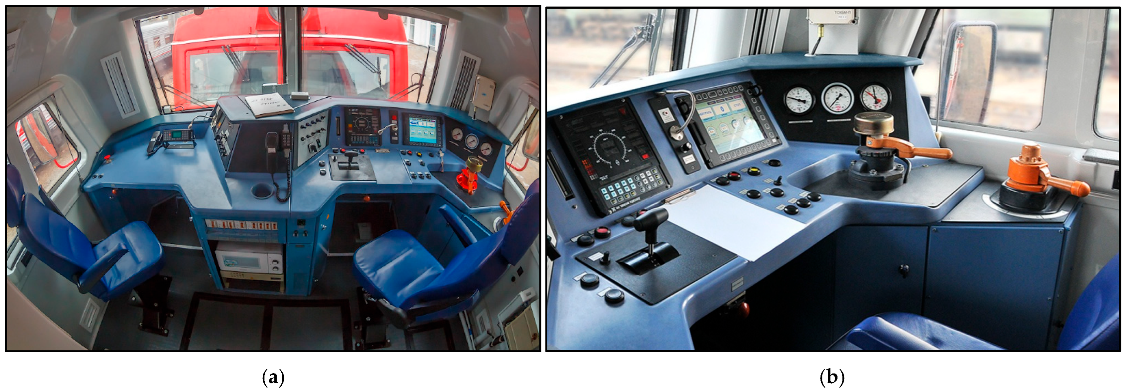
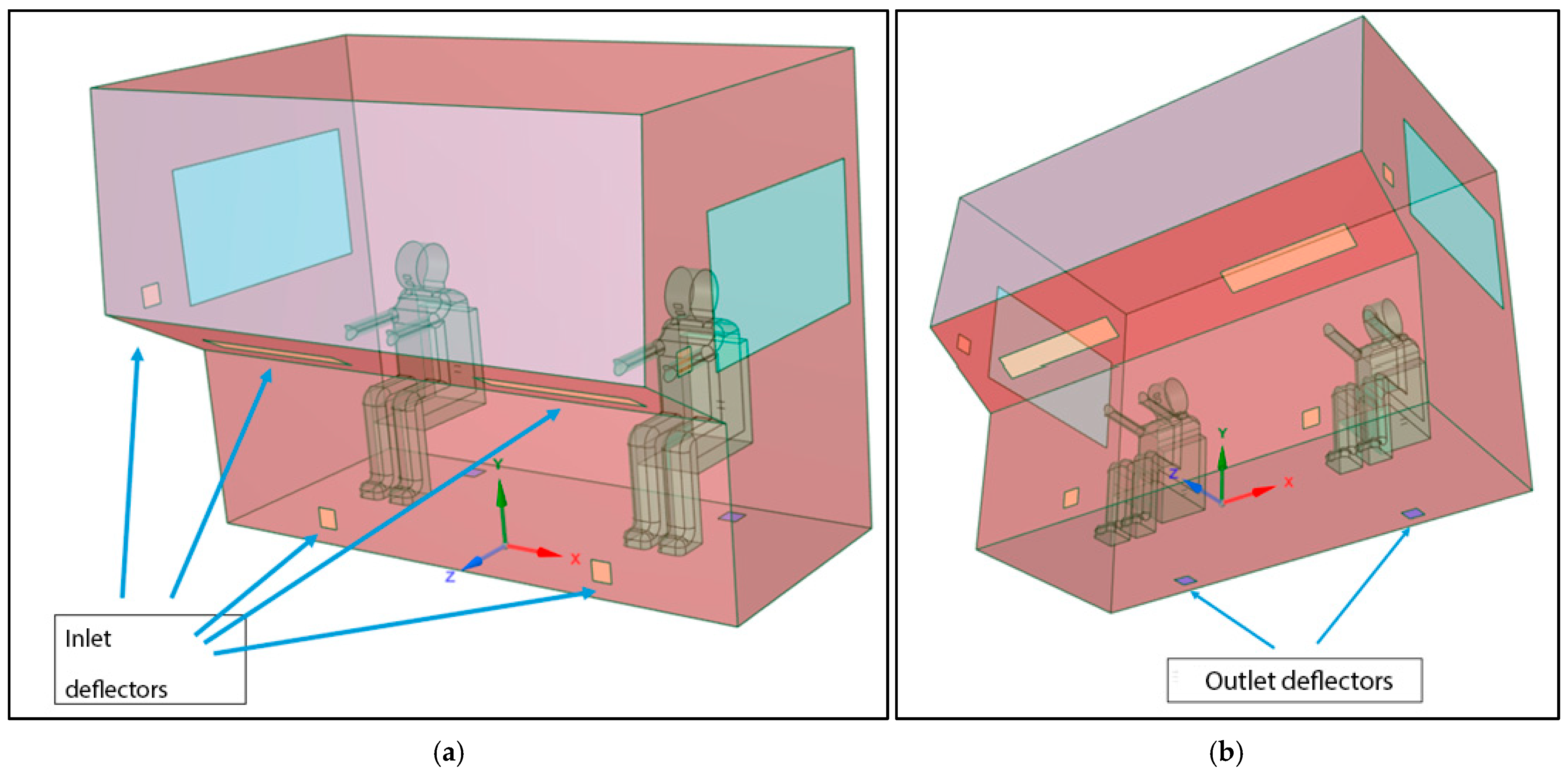
The experimental data were obtained from the test results for the 2TE25K diesel locomotive cabin (Figure 1) from “Protocol No. 125/1 for measuring microclimate indicators at workplaces dated 25 September 2020”, conducted by the Scientific and Production Center “Occupational Safety” of the ONIITS NICh RGUPS for summer mode.
The microclimate parameter meter “Meteoscope-M” [47] (Figure 2) was used to measure the microclimate parameters (Figure 2, serial No. 220516, ENKOR “Kauchuk” measuring tape, serial No. 799). Measurement and analysis methods: MUK 4.3.2756-10 SanPiN 2.2.4.548-96 [10].

2.3. Geometry Model

Figure 2 shows a prepared three-dimensional geometric model of the internal air domain of the cabin, the walls of which are the internal walls of the cabin of the 2TE25K diesel locomotive [48]. The inlet deflectors through which air enters the cabin are shown in orange in Figure 3a; the outlet deflectors through which air leaves the cabin are shown in blue in Figure 3b.

3. Results and Discussion

3.1. Numerical Analysis

The system of differential Equations (1)–(9) was solved numerically using the volume element method [33] in the Ansys CFD software (v. 2024 R2) product. In this case, Equations (1)–(9) are reduced to the RANS (Reynolds-Averaged Navier–Stokes) system using Reynolds averaging [49,50], equations with the addition of additional relations (turbulence equations) [49]. The essence of the Reynolds averaging method is that unknown quantities in a turbulent flow can be represented as the sum of the averaged quantity and the pulsation component [17,18,19]. To close the equations in this work, a turbine-lensed model with two differential equations kε was used, where the kinetic energy of turbulence k and the speed of dissipation of kinetic energy ε were the permanent unknown:
ρ k t + x j ρ u j k = P k ρ ε + x j μ + μ T σ k k x j
ρ ε t + x j ρ u j ε = ε k C ε 1 P k C ε 2 ρ ε + x j μ + μ T σ ε ε x j
P k = ρ u i u j u i x j ¯
μ T = η T ρ
η T = C μ k 2 ε
where σ k , σ ε , C ε 1 , C ε 2 , and C µ are constants, which should be predetermined from the calibration experiment [49]: σ k = 1 , σ ε = 1.3 , C ε 1 = 1.44 , C ε 2 = 1.92 , C µ = 0.09 .
After applying Reynolds averaging to the Navier–Stokes equations, the Reynolds-Averaged Navier–Stokes (RANS) for the steady-state case or URANS (unsteady RANS) equations for the unsteady case are obtained.
The model was divided into polygonal elements (see Figure 4b), which is quite effective for three-dimensional objects compared to tetragonal (Figure 4a) and cubic elements, since it allows the number of partition cells to be reduced. Half of the cabin was considered; the axis of symmetry divides the cabins in half between the drivers. For comparison, Table 1 and Figure 4a,b show the parameters of the tetragonal and polygonal mesh.
A series of test calculations was performed to verify the grid. Table 2 shows the results of differences in temperature values for five points in the cross section shown in Figure 4 with summer mode. The temperature values for the first combination of grid parameters were taken as 1, and, for the other combinations of grid parameters, the values were compared with the initial values at the corresponding points.
Table 3 shows the parameters of the numerical methods used in the calculation.

3.2. Task Parameters

To simulate the external heat exchange of the cabin with the environment through the wall and windows, a convective heat exchange model was employed using the applied Jurgens formula [16,51,52], for which the heat transfer coefficient is calculated according to Formula (16), and the boundary condition on the inner wall (which coincides with the outer surface of the inner air domain) is specified in the form of a heat flux:—   λ T n | Ω = q * = α T T o u t (where T o u t is the external air temperature, which is specified in Table 3, line 4). Based on their relationship (10), the heat transfer coefficients α through the wall into the environment were calculated as follows:
α = 1 i = 1 n δ i λ i + 1 5 + 3.4 u
where u is the external air flow velocity (train speed), λ i is the thermal conductivity of the i-th layer of the multilayer wall, and δ i is the thermal conductivity coefficient of the i-th layer of the multilayer wall. Table 4. Parameter values are given in Table 2.
For the parameters specified in Table 4 and the train speed of 27.8 m/s, the heat transfer coefficient for the multilayer wall was 1.04 W/(m2×K), and that of the windows was 45.34 W/(m2×K).
The heat transfer in a train moving at a constant speed of 27.8 m/s (100 km/h) in the summer (hot) and cool periods was considered in the numerical experiments. The initial and boundary conditions are specified in Table 5. The film thickness and temperature at the initial time are set as the initial condensation parameters.
To determine the numerical values of the mass and thermal diffusion coefficients from Equation (6), the kinetic theory available in Ansys Fluent [33] was used. The averaged values are given in Table 5.

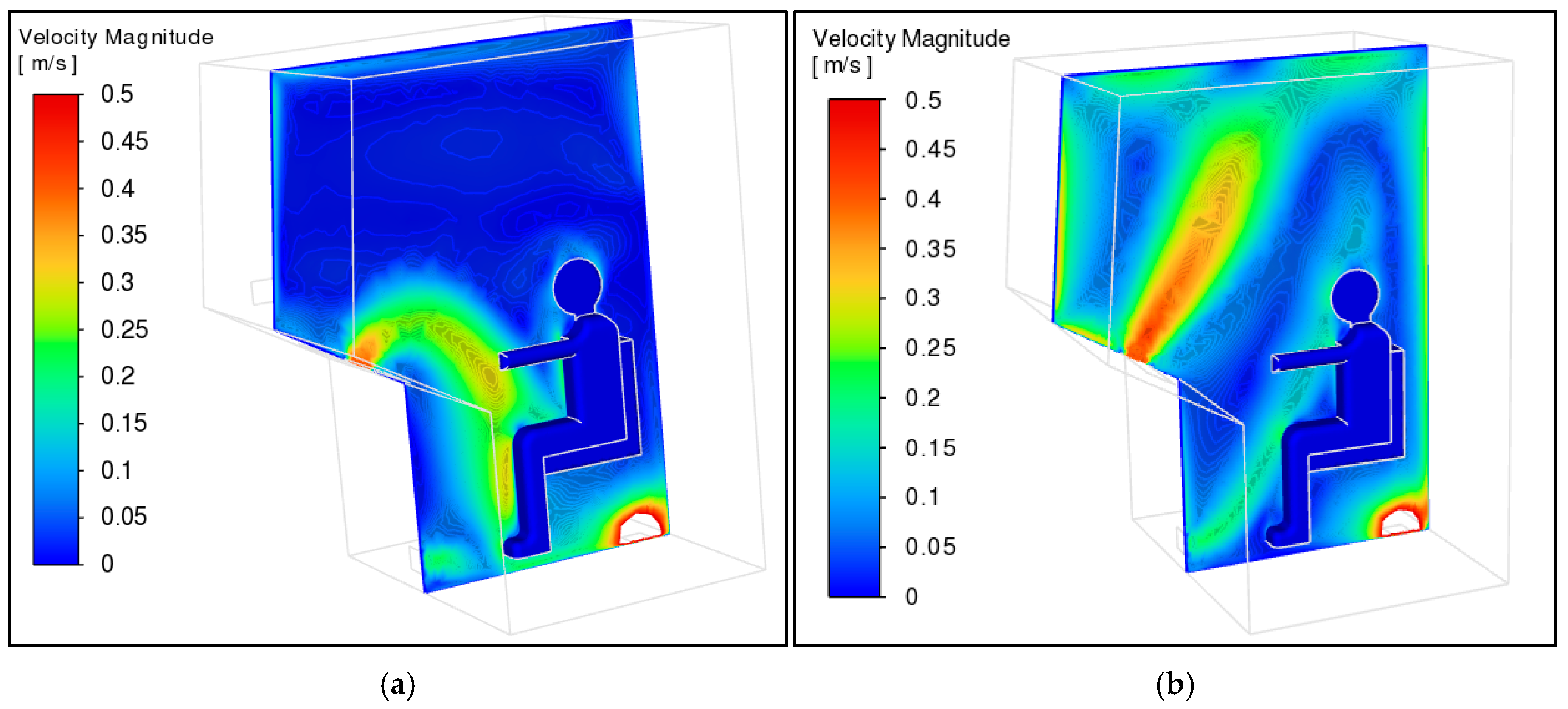
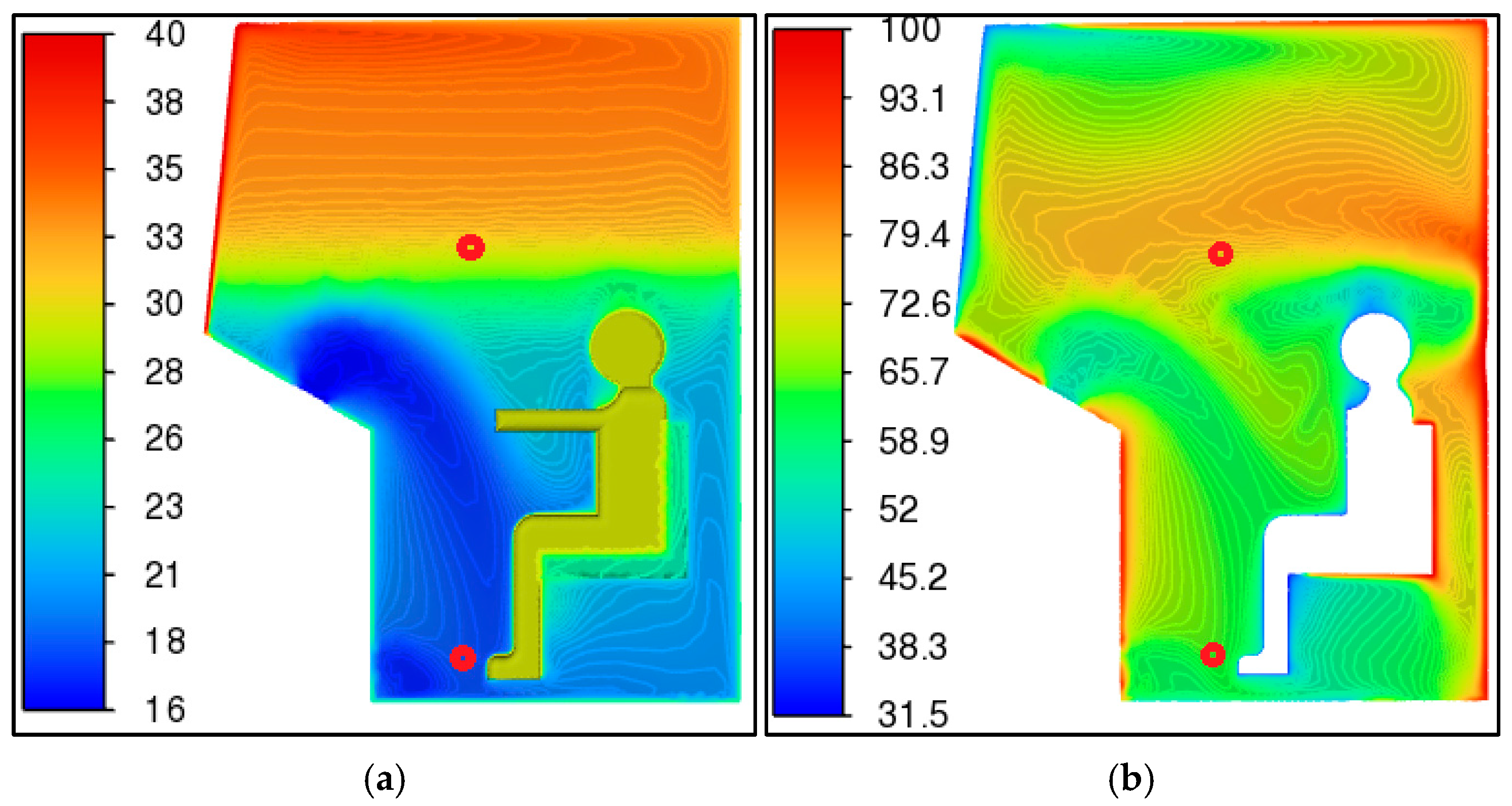
3.3. Numerical Results for Temperature and Air Speed and Verification of Results

The following graphs show the simulation results for the temperature and air velocity fields at a time value of 300 s, for which the values stabilize.
Figure 5, Figure 6 and Figure 7 show the velocity and temperature fields for the summer and cool periods for a plane passing through the middle of the driver. The stabilized average temperature value for the summer mode was 25.2 °C, and for the cool mode it was 22.6 °C. Temperature fields have severe heterogeneity for the specified time of the climatic system due to the gradient of the temperature of the incoming flow and internal air.
Figure 8 additionally show fields of turbulence intensity for different ranges of values (at different scales).

3.4. Verification and Comparison with Experimental Data

To verify the results and check the numerical model, the results of temperature modeling were compared with the study conducted in [47] without taking into account the condensation model for the summer period. Temperature comparison graphs are shown in Figure 9 for the summer period. The difference in the result for a time of 300 s was about 12.5%. The temperature values with the condensation model taken into account are lower than without it, since part of the thermal energy is spent on the evaporation process (thermal energy is spent on the kinetic energy of liquid molecules, on the transformation from a liquid to a gaseous state).
The temperature comparison graphs with and without the condensation model are shown in Figure 10 for the cool period. The difference in the result for 300 s was about 9.6%. The temperature values with the condensation model are lower than without it. As shown below, this is also because of the complex process of evaporation and condensation of moisture from surfaces (Figure 10).
To compare the obtained results with the experimental data, temperature and humidity measurements were taken at characteristic points (Figure 11a,b, red dots) in the cabin of the 2TE25K diesel locomotive. Based on the measurement results, “Protocol No. 125/1 for measuring microclimate indicators at workplaces dated 25 September 2020” was compiled, conducted jointly with the Scientific and Production Center “Occupational Safety” of the ONIITS NICh RGUPS for the summer mode. The temperature regimes and atmospheric conditions obtained theoretically and experimentally are given in accordance with Table 5 for the summer mode.
According to these methods, measurements are taken in the driver’s and assistant driver’s areas at a distance of 0.15 m and 1.5 m from the floor level, and the average temperature and humidity values are recorded in the protocol (Figure 11a,b). The declared error in measuring temperature is ±0.2 °C, and the relative humidity is ±3%.
Thus, Table 6 shows the data of the numerical calculations of temperature and humidity, as well as experimental data.
As shown in Table 6, the error for temperature considering the condensation model is 11%; without taking into account the condensation model, the value is 18%. For relative humidity, considering the condensation model yields a value of 16%; without taking into account the condensation model, the value is 29%.

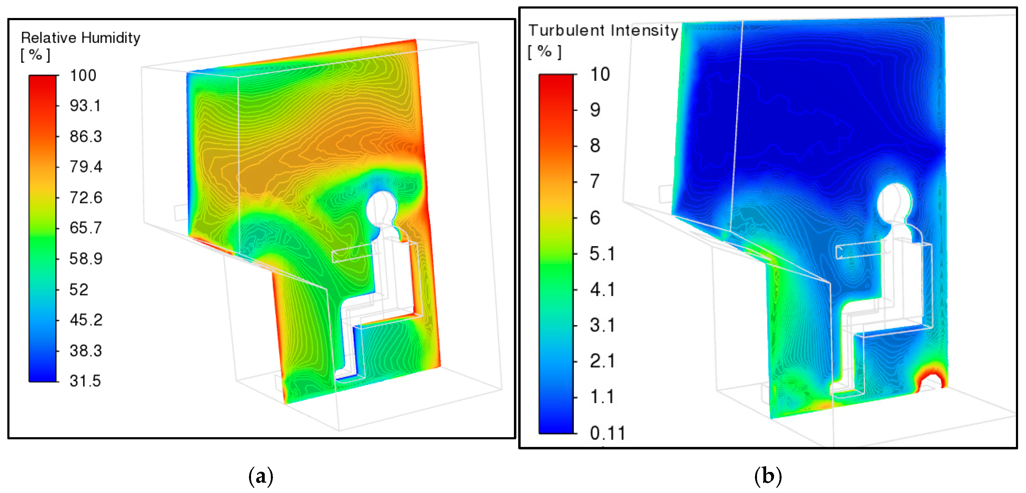
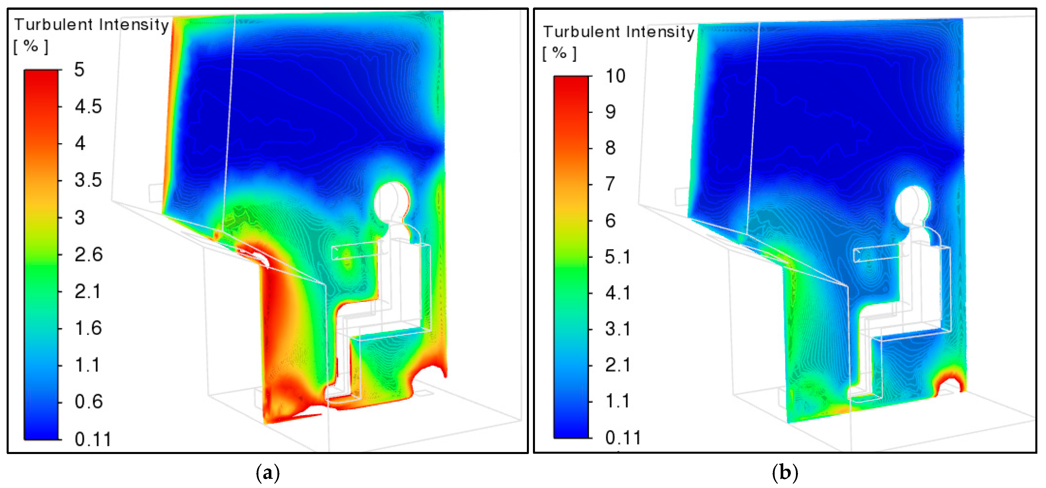
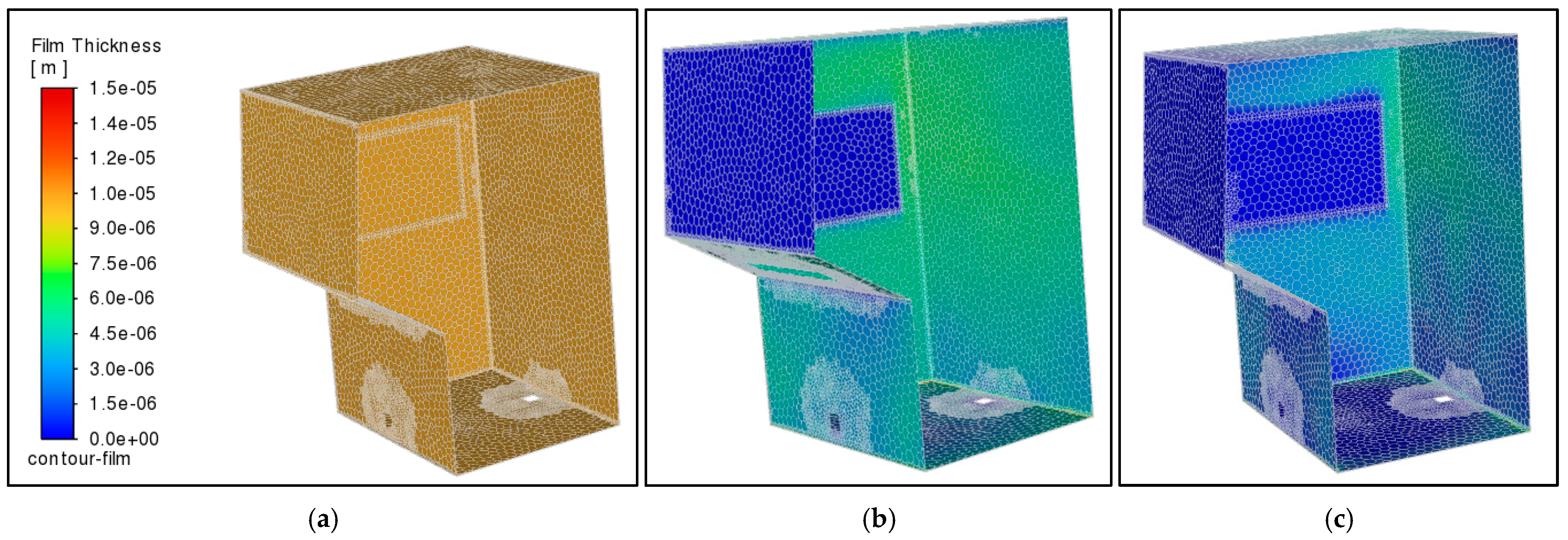
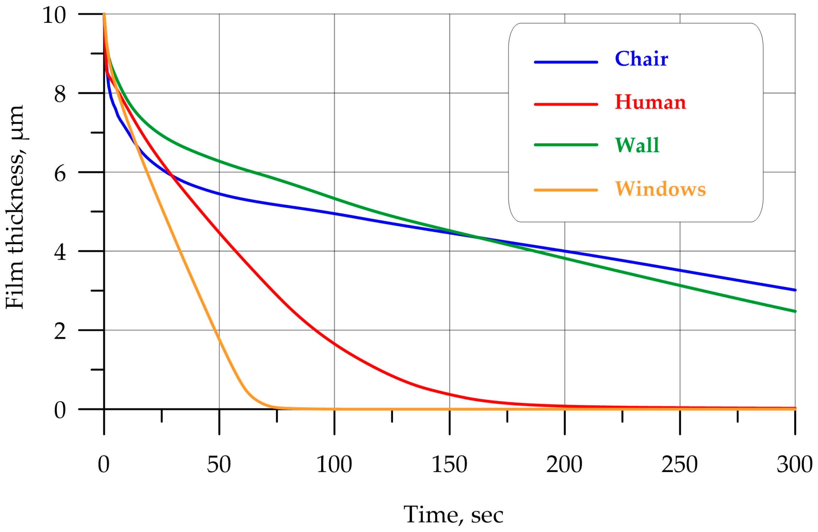
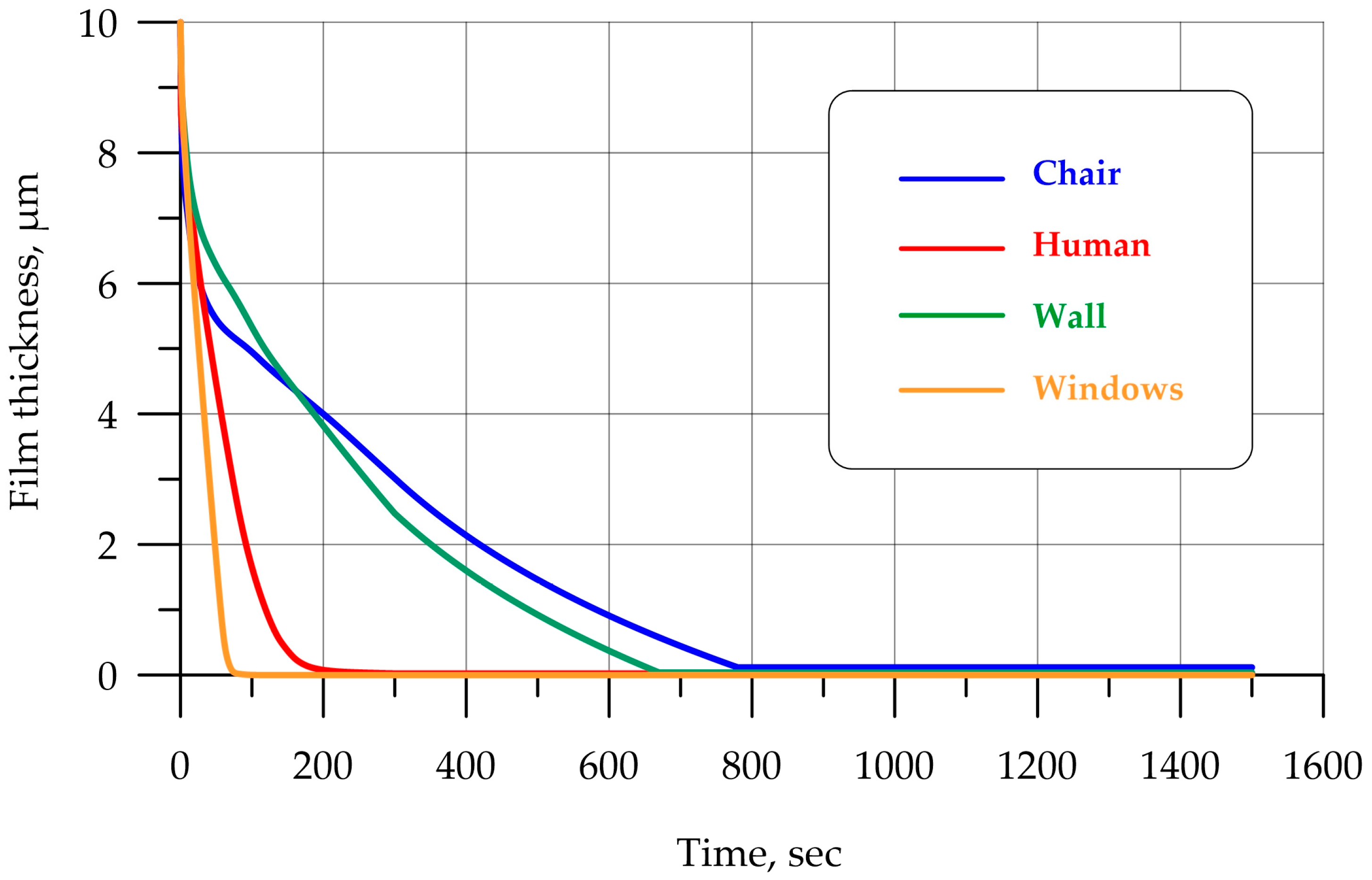
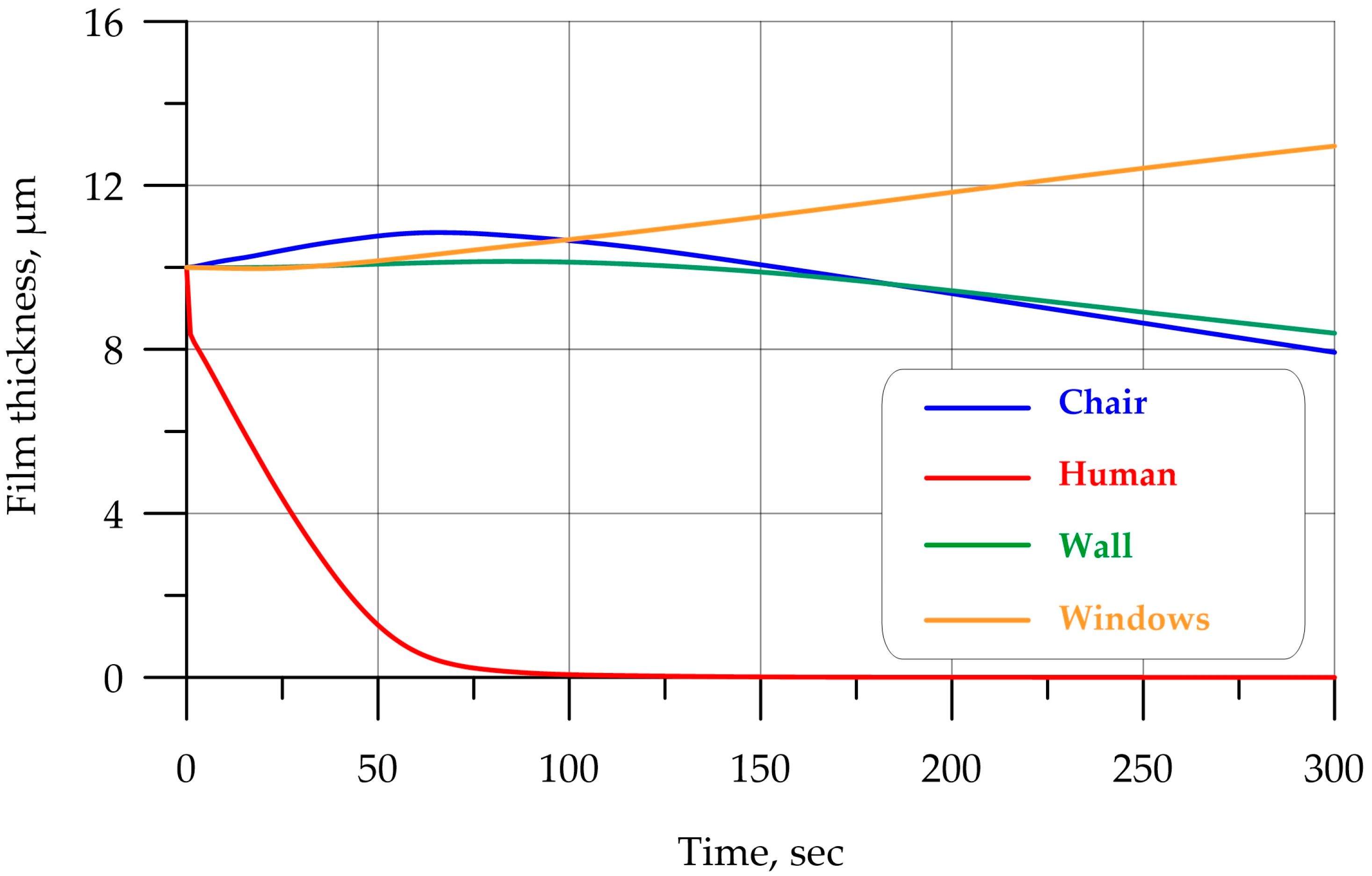
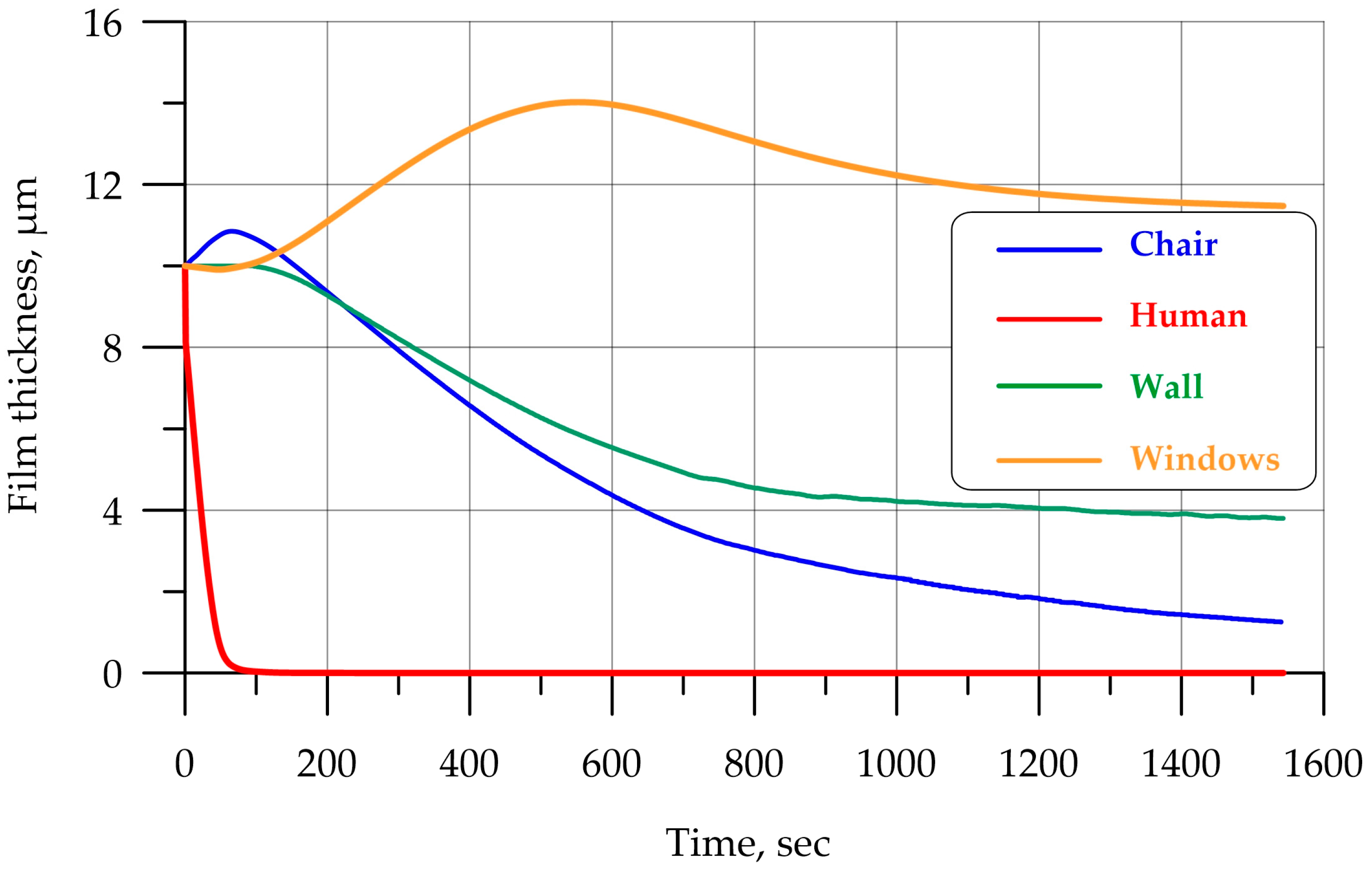
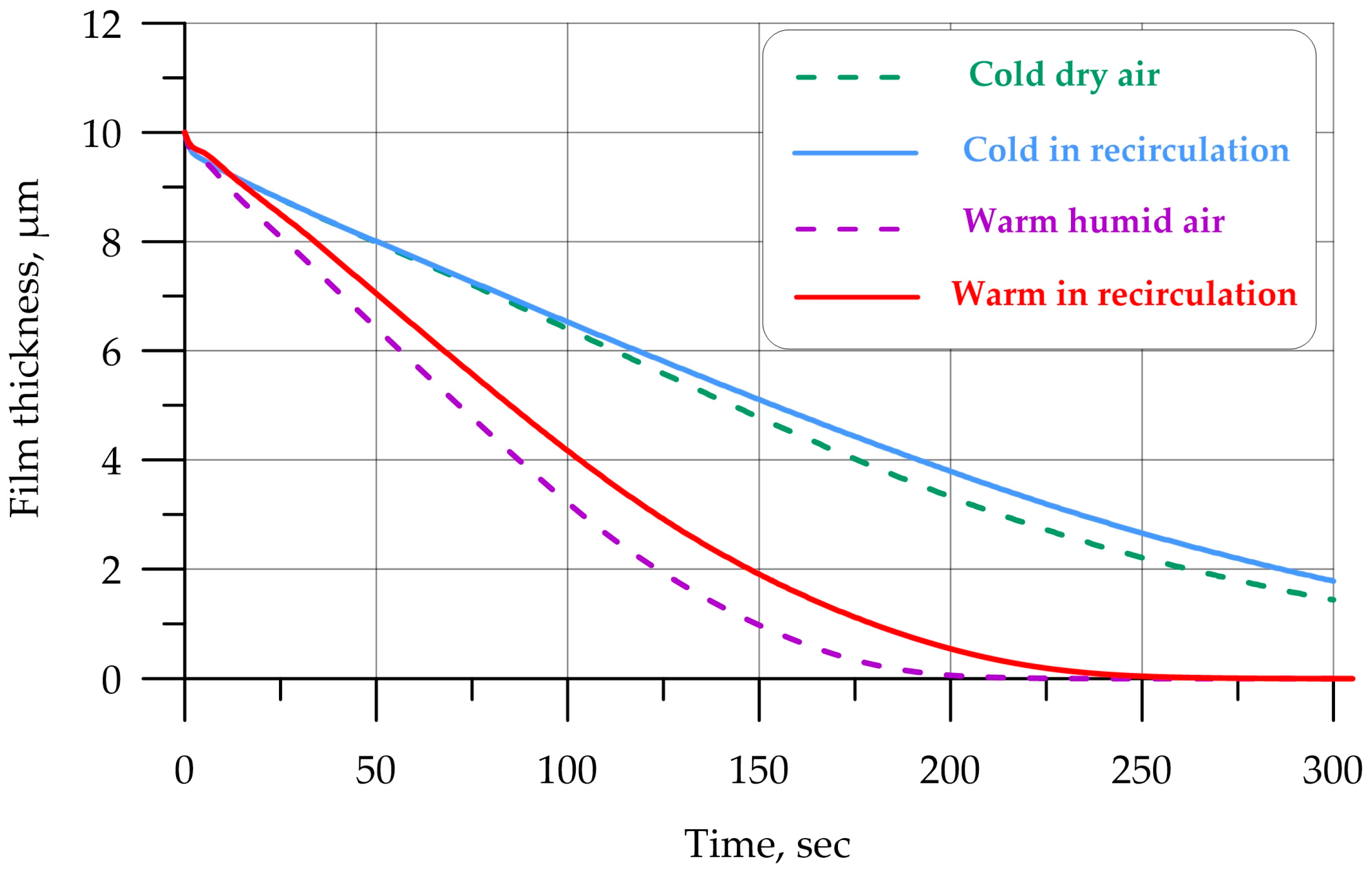
3.5. Numerical Results for Humidity and Condensation for Different Circulation Regimes: Discussion of Results

Numerical results of humidity and condensation film fields for different air circulation regimes are presented below.
Figure 12 shows the results of moisture film thicknesses on walls and windows at different points in time for the summer mode. Figure 13 shows the graphs of average film thicknesses on all surfaces for 300 s; Figure 14 shows the graphs of average film thicknesses on all surfaces for 1500 s. On the surface of a person and window surfaces, evaporation occurs much faster than on the surfaces of walls and the surface of a chair. This fact is explained by the much higher temperatures on the surfaces of windows and a person than on the others.
Modeling condensation on the surface of a chair (heat flux is zero) was added intentionally. In this way, it is possible to model other surfaces inside the cabin: for example, the instrument panel, etc.
Figure 13 shows that, after 200 s, the film thickness on the surface of the person and windows (the hottest surfaces) becomes zero—that is, the film evaporates. On the surface of the chair and interior walls, the film thickness decreases much more slowly.
Figure 15 shows the results of moisture film thicknesses on walls and windows at different points in time for the cool mode. Figure 16 shows the graphs of average film thicknesses on all surfaces for 300 s, and Figure 17 shows the graphs of average film thicknesses on all surfaces for 1500 s. Here, the distribution pattern of condensed moisture over time is significantly non-uniform: on the surface of a person, the film thickness decreases, on the surface of windows, the film thickness increases, and, on the surfaces of walls and steel, the film thickness increases up to 60 s and then decreases. This is due to the non-uniformity of temperature values on different surfaces: there are both heated surfaces (people) and those with temperatures low enough (window surfaces) for condensation to form.
Additionally, in this study, a numerical experiment was simulated to determine the most effective mode of condensate removal from the window surface. In the first mode, cool air with a minimum moisture content is blown (cooled air from the air conditioning system with low humidity due to the evaporator radiator). In the second mode, heated air with high humidity is blown (heated atmospheric from the climate system). The parameters are given in Table 7. Additionally, the recirculation modes were investigated: in these modes, the humidity at the inlet was set equal to the humidity at the outlet starting from the second iteration, the other air parameters were set according to Table 7. The condensate removal rate is compared for both modes.
The dependences of the average thicknesses of condensation films are shown in Figure 18.
As shown in Figure 18, blowing with heated air showed more effective results for these parameters than blowing with cooled “dry” air. For dry air, the film thickness decreases by 83% at a time value of 300 s; for warm, more humid air, the film thickness decreases almost to zero (i.e., the film evaporates completely). For recirculation modes, slower condensate removal is noticeable: for the cold mode, the difference between circulation and recirculation mode reaches an average of 9.2%, and, for the warm mode, the value is 17.4%. This finding is quite interesting and allows for the more efficient control of condensate removal from the cabin surfaces.
Similar studies in this area for transportation cabins have been carried out [40,41,42,43,44,46,53]. For example, in [54], the air conditioning process in a vehicle and the elimination of fogging were investigated using the Eulerian Wall Film model. The authors studied different conditions of the temperature, humidity and velocity of incoming ventilation air and found that the mass flow rate, inlet temperature and humidity directly affect the dew film thickness. A flow temperature of 46.85 °C shows the highest condensate removal efficiency, which is almost the same as the results of the optimum flow temperature of 45 °C obtained in the present study.

4. Conclusions

This work is devoted to the study of the formation and removal of condensate from the surfaces of the transport cabin, as well as the effect of condensation on the parameters of the microclimate—in particular, temperature.
Based on the fundamental Navier–Stokes equations and energy and diffusion equations, a mathematical model of the thermodynamic fields of temperature, velocity, pressure and concentration of moisture vapor inside the cabin was constructed. Using the Euler Film Model, the formation and removal of moisture on the surfaces of the cabin was simulated as a phase transition from the gaseous state to the liquid state and back. In this case, all the microclimate fields are related. The problem was solved numerically based on averaging the variables according to Reynolds and applying the turbulence model using the volume element method in the Ansys CFD software product. Numerical experiments were conducted for two climatic conditions of the external environment (warm and cold external air) for the cabin of the mainline two-section diesel locomotive: at the initial moment of time, the presence of a condensate film was specified, and further evaporation or condensation of the film was considered. The following main results were obtained:
Related fields of temperature, velocity and moisture concentration were constructed for different time intervals, and dependences of film thicknesses on different surfaces on time were found;
Verification was carried out with the results of other studies, without taking into account the phase transition and condensation: for example, for the warm mode, the average air temperature in the cabin turns out to be 12.5% lower when taking into account condensation than without taking into account condensation, which is associated with the process of evaporation of liquid from heated walls. For the cold mode, the evaporation process turned out to be non-uniform: moisture evaporates from some hotter walls, while moisture condenses from other cooler ones (in particular, windows). Overall, the difference in temperature values with and without the condensation model ranged from −12.5% to +4.9%;
A comparison was made with experimental data based on the protocol for measuring microclimate indicators at workplaces for the train cabin: the average error for temperature ranged from 11% to 18% and for relative humidity it ranged from 16% to 26% for different models. Taking into account the condensation model showed the closest results relative to the experiment.
A numerical experiment was also conducted to assess the most effective method for the removal of condensate film from the window surface: for the given parameters, blowing with warm humid air removes condensate faster than blowing with cold, drier air.
Thus, taking into account the moisture condensation model can significantly affect, among other things, the parameters of the microclimate in cabins—in particular, temperature. The application of numerical modeling is required, simultaneously with the basic heat transfer equations.
We propose that future studies add a model of the phase transition of water vapor inside the innermost domain of the cabin. In particular, based on multiphase models, for example, VOF or Ehler, it is possible to model the formation and transfer of water vapor throughout the cabin volume and also to compare it with the Euler Film Model.

Author Contributions

Conceptualization, I.P. and A.N.B.; methodology, I.P. and A.N.B.; software, I.P.; validation, I.P. and A.N.B.; formal analysis, I.P.; investigation, I.P., A.N.B., S.F.P. and B.M.; resources, B.M.; data curation, I.P. and S.F.P.; writing—original draft preparation, I.P. and A.N.B.; writing—review and editing, I.P. and A.N.B.; visualization, I.P.; supervision, B.M.; project administration, B.M.; funding acquisition, A.N.B. and B.M. All authors have read and agreed to the published version of the manuscript.

Funding

This research received no external funding.

Institutional Review Board Statement

Not applicable.

Informed Consent Statement

Not applicable.

Data Availability Statement

The original contributions presented in this study are included in the article. Further inquiries can be directed to the corresponding author.

Acknowledgments

The authors would like to acknowledge the administration of Don State Technical University for their resources and financial support.

Conflicts of Interest

The authors declare no conflicts of interest.

References

  1. Transport in Russia. 2022: Stat. Collection/Rosstat.—T65 M., 2022—101p. Available online: https://mintrans.gov.ru/file/504718 (accessed on 11 March 2025).
  2. Federal State Statistics Service. [Electronic Resource]. Available online: https://rosstat.gov.ru/statistics/transport (accessed on 11 March 2025).
  3. Li, X.; Patel, M.J.; Cole, I.S. Portable Air Purifiers’ Predicted Efficacy in Mitigating Airborne Pathogen Transmission in an Office Room Featuring Mixing Ventilation. Fluids 2023, 8, 307. [Google Scholar] [CrossRef]
  4. Pozevalkin, V.V.; Polyakov, A.N. Implementation of a Digital Model of Thermal Characteristics Based on the Temperature Field. Adv. Eng. Res. 2024, 24, 178–189. [Google Scholar] [CrossRef]
  5. Yao, J.; Yao, Y. Transient CFD Modelling of Air–Water Two-Phase Annular Flow Characteristics in a Small Horizontal Circular Pipe. Fluids 2022, 7, 191. [Google Scholar] [CrossRef]
  6. Moveh, S.; Merchán-Cruz, E.A.; Ibrahim, A.O.; Elhassan, Z.A.M.; Ramadan Abdelhai, N.M.; Abdelrazig, M.D. Thermodynamic Optimization of Building HVAC Systems Through Dynamic Modeling and Advanced Machine Learning. Sustainability 2025, 17, 1955. [Google Scholar] [CrossRef]
  7. ANSI ANSI/ASHRAE Standard 62.1-2010, Ventilation for Acceptable Indoor Air Quality. Available online: https://www.ashrae.org/technical-resources/bookstore/standards-62-1-62-2 (accessed on 11 March 2025).
  8. ANSI/ASHRAE Standard 55-2017 Thermal Environmental Conditions for Human Occupancy. Approved by ASHRAE and the American National Standards Institute on 31 July 2020. Available online: https://clck.ru/3ESQGh (accessed on 11 March 2025).
  9. Safety Standards for Railway Transport Electric Locomotives. NB ZhT CT 04-98 Electric Locomotives. Safety Standards. - M.: 1998. -123p. Available online: https://files.stroyinf.ru/Data2/1/4293756/4293756801.pdf (accessed on 11 March 2025).
  10. Resolution of the Chief State Sanitary Doctor of the Russian Federation dated 28 January 2021 No. 2 On Approval of Sanitary Rules and Regulations SANPIN 1.2.3685-21 "Hygienic Standards and Requirements for Ensuring the Safety and (or) Harmlessness of Environmental Factors for Humans". [Electronic Resource]. Available online: https://base.garant.ru/400274954/ (accessed on 25 July 2025).
  11. Mikheev, M.A.; Mikheeva, I.M. Fundamentals of Heat Transfer, 2nd ed.; Energia: Moscow, Russia, 1977; 344p. [Google Scholar]
  12. Sapozhnikov, S.Z.; Kitanin, E.L. Engineering Thermodynamics and Heat Transfer; Publishing House: St. Petersburg, Russia, 2001; 317p. [Google Scholar]
  13. Saghir, M.Z.; Rahman, M.M. Effectiveness in Cooling a Heat Sink in the Presence of a TPMS Porous Structure Comparing Two Different Flow Directions. Fluids 2024, 9, 297. [Google Scholar] [CrossRef]
  14. Panfilov, I.A. Study of heat transfer in shell-and-tube heat exchangers using stored refrigerant. XXI Century: Results Past Probl. Present Plus 2024, 13, 181–188. [Google Scholar]
  15. Mokrane, M.; Bourouis, M. Heat Transfer and Fluid Flow Characteristics in a Micro Heat Exchanger Employing Warm Nanofluids for Cooling of Electronic Components. Energies 2024, 17, 2383. [Google Scholar] [CrossRef]
  16. Beskopylny, A.N.; Panfilov, I.; Meskhi, B. Modeling of Flow Heat Transfer Processes and Aerodynamics in the Cabins of Vehicles. Fluids 2022, 7, 226. [Google Scholar] [CrossRef]
  17. Taebi, A. Deep Learning for Computational Hemodynamics: A Brief Review of Recent Advances. Fluids 2022, 7, 197. [Google Scholar] [CrossRef]
  18. Pioch, F.; Harmening, J.H.; Müller, A.M.; Peitzmann, F.-J.; Schramm, D.; el Moctar, O. Turbulence Modeling for Physics-Informed Neural Networks: Comparison of Different RANS Models for the Backward-Facing Step Flow. Fluids 2023, 8, 43. [Google Scholar] [CrossRef]
  19. Drikakis, D.; Sofos, F. Can Artificial Intelligence Accelerate Fluid Mechanics Research? Fluids 2023, 8, 212. [Google Scholar] [CrossRef]
  20. Zhou, X.-W.; Liu, F.-T.; Jin, Y.-F.; Yin, Z.-Y.; Zhang, C.-B. A volumetric locking-free stable node-based smoothed finite element method for geomechanics. Comput. Geotech. 2022, 149, 104856, ISSN 0266-352X. [Google Scholar] [CrossRef]
  21. Quaresma, A.L.; Romão, F.; Pinheiro, A.N. A Comparative Assessment of Reynolds Averaged Navier–Stokes and Large-Eddy Simulation Models: Choosing the Best for Pool-Type Fishway Flow Simulations. Water 2025, 17, 686. [Google Scholar] [CrossRef]
  22. Andrew, S. Kowalski, Jesús Abril-Gago, Exploring unresolved inquiries regarding the meaning of Reynolds averaging and decomposition: A review. Agric. For. Meteorol. 2025, 362, 110364, ISSN 0168-1923. [Google Scholar] [CrossRef]
  23. Chen, X.; Ishihara, T. Numerical study of turbulent flows over complex terrain using an unsteady Reynolds-averaged Navier-Stokes model with a new method for turbulent inflow generation. J. Wind. Eng. Ind. Aerodyn. 2025, 257, 105991, ISSN 0167-6105. [Google Scholar] [CrossRef]
  24. Li, Z.; Zhou, T.; Lu, W.; Yang, H.; Li, Y.; Liu, Y.; Zhang, M. Computational Fluid Dynamics (CFD) Technology Methodology and Analysis of Waste Heat Recovery from High-Temperature Solid Granule: A Review. Sustainability 2025, 17, 480. [Google Scholar] [CrossRef]
  25. Yee, H.C.; Sweby, P.K.; Sjögreen, B.; Kotov, D.V. A Nonlinear Approach in the Quantification of Numerical Uncertainty by High-Order Methods for Compressible Turbulence with Shocks. Fluids 2024, 9, 250. [Google Scholar] [CrossRef]
  26. Tong, K.; Yang, L.; Du, X.; Yang, Y. Review of modeling and simulation strategies for unstructured packing bed photoreactors with CFD method. Renew. Sustain. Energy Rev. 2020, 131, 109986, ISSN 1364-0321. [Google Scholar] [CrossRef]
  27. Panfilov, I.; Beskopylny, A.N.; Meskhi, B. Improving the Energy Efficiency of Vehicles by Ensuring the Optimal Value of Excess Pressure in the Cabin Depending on the Travel Speed. Fluids 2024, 9, 130. [Google Scholar] [CrossRef]
  28. Ogundiran, J.O.; Nyembwe, J.-P.K.B.; Ogundiran, J.; Ribeiro, A.S.N.; Gameiro da Silva, M. A Systematic Review of Indoor Environmental Quality in Passenger Transport Vehicles of Tropical and Subtropical Regions. Atmosphere 2025, 16, 140. [Google Scholar] [CrossRef]
  29. Luger, C.; Kallinovsky, J.; Rieberer, R. Identification of representative operating conditions of HVAC systems in passenger rail vehicles based on sampling virtual train trips. Adv. Eng. Inform. 2016, 30, 157–167, ISSN 1474-0346. [Google Scholar] [CrossRef]
  30. Pan, D.; Wen, D.; Guo, X.; Song, H.; Bai, S. Factors Influencing the Sterilization of E. coli in a High-Voltage Electric Field: Electric Field Strength, Temperature and Humidity. Processes 2025, 13, 551. [Google Scholar] [CrossRef]
  31. Yang, Y.; Shi, N.; Zhang, R.; Zhou, H.; Ding, L.; Tao, J.; Zhang, N.; Cao, B. Study on the Effect of Local Heating Devices on Human Thermal Comfort in Low-Temperature Built Environment. Buildings 2024, 14, 3996. [Google Scholar] [CrossRef]
  32. Dixit, S.; Kumar, A.; Kumar, S.; Waghmare, N.; Harish; Thakur, C.; Khan, S. CFD analysis of biodiesel blends and combustion using Ansys Fluent. Mater. Today Proc. 2020, 26, 665–670, ISSN 2214-7853. [Google Scholar] [CrossRef]
  33. 33. Ansys Fluent Tutorial Guide 2023 R1. 2023. Canonsburg, PA. Available online: https://www.ansys.com/content/dam/amp/2023/december/quick-request/ansys-education-resources-23q4-part-1/intro-to-fluent-tutorial-tutiafflen24.pdf (accessed on 9 December 2024).
  34. Soloviev, A.N.; Panfilov, I.A.; Lesnyak, O.N.; Lee, C.Y.J.; Liu, Y.M. Numerical Simulation of Relative Humidity in a Vehicle Cabin. In Physics and Mechanics of New Materials and Their Applications; Parinov, I.A., Chang, S.H., Soloviev, A.N., Eds.; Springer Proceedings in Materials; Springer: Cham, Switzerland, 2023; Volume 20. [Google Scholar] [CrossRef]
  35. Lesage, M.; Chalet, D.; Migaud, J. Optimising Ventilation Strategies for Improved Driving Range and Comfort in Electric Vehicles. World Electr. Veh. J. 2025, 16, 98. [Google Scholar] [CrossRef]
  36. Jiang, Y.; Zhu, S.; Xu, Q.; Yang, B.; Guan, X. Hybrid modeling-based temperature and humidity adaptive control for a multi-zone HVAC system. Appl. Energy 2023, 334, 120622, ISSN 0306-2619. [Google Scholar] [CrossRef]
  37. Raman, N.S.; Devaprasad, K.; Chen, B.; Ingley, H.A.; Barooah, P. Model predictive control for energy-efficient HVAC operation with humidity and latent heat considerations. Appl. Energy 2020, 279, 115765, ISSN 0306-2619. [Google Scholar] [CrossRef]
  38. Panfilov, I.; Beskopylny, A.N.; Meskhi, B. Numerical Simulation of Heat Transfer and Spread of Virus Particles in the Car Interior. Mathematics 2023, 11, 784. [Google Scholar] [CrossRef]
  39. Annapeh, H.F.; Kurushina, V.A. Analysis of the Drag-Reduction Ability of the Layout and Cross-Sectional Shapes of Subsea Structures in the Critical Flow Mode. Adv. Eng. Res. 2024, 24, 135–147. [Google Scholar] [CrossRef]
  40. Zhang, J.; Chen, Q.; Liu, J.; Wang, Y.; Zhou, H.; Yang, F.; Ru, Y. Experiments and CFD simulation of downwash airflow and fog distribution discharged from a single-rotor UAV fitted with a pulse-jet thermal fogging machine. Biosyst. Eng. 2024, 240, 142–151, ISSN 1537-5110. [Google Scholar] [CrossRef]
  41. George, A.; Kelm, S.; Cheng, X.; Allelein, H.-J. Efficient CFD modelling of bulk condensation, fog transport and re-evaporation for application to containment scale. Nucl. Eng. Des. 2023, 401, 112067, ISSN 0029-5493. [Google Scholar] [CrossRef]
  42. Kim, J.; Kang, J. AI based temperature reduction effect model of fog cooling for human thermal comfort: Climate adaptation technology. Sustain. Cities Soc. 2023, 95, 104574, ISSN 2210-6707. [Google Scholar] [CrossRef]
  43. Nisa, E.C.; Lee, Y.; Kuan, Y.-D. Machine learning-based modeling and fogging prevention strategies for ice rink environments. Build. Environ. 2024, 258, 111553, ISSN 0360-1323. [Google Scholar] [CrossRef]
  44. Babu, A.R.; Sebben, S.; Chronéer, Z.; Etemad, S. An adaptive cabin air recirculation strategy for an electric truck using a coupled CFD-thermoregulation approach. Int. J. Heat Mass Transf. 2024, 221, 125056, ISSN 0017-9310. [Google Scholar] [CrossRef]
  45. Hou, J.; Li, S.; Pan, W.; Yang, L. Co-Simulation Modeling and Multi-Objective Optimization of Dynamic Characteristics of Flow Balancing Valve. Machines 2023, 11, 337. [Google Scholar] [CrossRef]
  46. D’Agaro, P.; Croce, G.; Cortella, G. Numerical simulation of glass doors fogging and defogging in refrigerated display cabinets. Appl. Therm. Eng. 2006, 26, 1927–1934, ISSN 1359-4311. [Google Scholar] [CrossRef]
  47. Panfilov, I.; Beskopylny, A.N.; Meskhi, B. Improving the Fuel Economy and Energy Efficiency of Train Cab Climate Systems, Considering Air Recirculation Modes. Energies 2024, 17, 2224. [Google Scholar] [CrossRef]
  48. JSC Transmashholding. Main-Line Freight Diesel Locomotive 2TE25K: [Electronic Resource]. Available online: https://tmholding.ru/products/gruzovye/teplovozy-2te25km-3te25k2m/ (accessed on 3 March 2025).
  49. Pope, S. Turbulent Flows; Cambridge University Press: Cambridge, UK, 2000; 771p. [Google Scholar]
  50. Landau, L.D.; Lifshits, E.M. Course of Theoretical Physics; Hydrodynamics. M.: Nauka, Mexico, 1988; Volume 6, 736p. [Google Scholar]
  51. Kuzovlev, V.A. Technical Thermodynamics and Fundamentals of Heat Transfer, 2nd ed.; Vysshaya Shkola: Moscow, Russia, 1983; 335p. [Google Scholar]
  52. Kutateladze, S.S. Heat Transfer and Hydrodynamic Resistance: Reference Manual; Energoatomizdat: Moscow, Russia, 1990; 367p. [Google Scholar]
  53. Yang, Y.; Huang, Y.; Zhao, J. Optimization of the automotive air conditioning strategy based on the study of dewing phenomenon and defogging progress. Appl. Therm. Eng. 2020, 169, 114932, ISSN 1359-4311. [Google Scholar] [CrossRef]
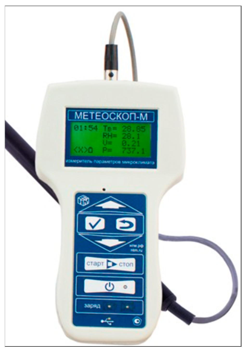
  54. METEOSCOP-M Meter of Microclimate Parameters. [Electronic Resource]. Available online: https://ntm.ru/products/70/7774 (accessed on 25 July 2025).
Figure 1. 2TE25KM: cabin of a two-section mainline freight locomotive 2TЭ25K: (a) general view; (b) control system [48].
Fluids 10 00197 g001
Figure 2. Meteoskop-M.
Fluids 10 00197 g002
Figure 3. 2TE25KM—cabin of the mainline two-section diesel locomotive 2TE25K. (a) Input deflectors; (b) output deflectors.
Fluids 10 00197 g003
Figure 4. Cabin: (a) finite volume grid—tetragonal grid; (b) finite volume grid—polygonal grid; (c) temperature field in the middle section.
Fluids 10 00197 g004
Figure 5. Temperature, °C: (a) summer mode, (b) winter mode.
Fluids 10 00197 g005
Figure 6. Velocity field, m/s: (a)—summer mode, (b)—winter mode.
Fluids 10 00197 g006
Figure 7. Relative humidity, %: (a)—summer mode, (b)—winter mode.
Fluids 10 00197 g007
Figure 8. Turbulence intensity for summer mode, %: (a) range: [0, 5], (b) range: [0, 10].
Fluids 10 00197 g008
Figure 9. Temperature values in °C for summer mode with and without condensation [47].
Fluids 10 00197 g009
Figure 10. Temperature values in °C for cool mode with and without condensation [47], with condensation on all surfaces, and without condensation on windows only.
Fluids 10 00197 g010
Figure 11. Numerical and experimental data comparison: (a) temperature °C and (b) relative humidity %; red circles indicate measurement points.
Fluids 10 00197 g011
Figure 12. The thickness of the condensed film on the surfaces of the wall and windows for summer mode for different moments in time: (a) time = 0 s; (b) time = 150 s; (c) time = 300 s.
Fluids 10 00197 g012
Figure 13. Average condensed film thickness values on cabin surfaces for summer mode depending on time, for a time of 300 s.
Fluids 10 00197 g013
Figure 14. Average condensed film thickness values on cabin surfaces for summer mode depending on time, for a time of 1500 s.
Fluids 10 00197 g014
Figure 15. Values of the thickness of the condensed film on the surfaces of the wall and windows for the cool mode for different moments in time: (a) time = 0 s; (b) time = 150 s; (c) time = 300 s.
Fluids 10 00197 g015
Figure 16. Average thickness values of the condensed film on the cabin surfaces for the cool mode depending on time, for a time of 300 s.
Fluids 10 00197 g016
Figure 17. Average thickness values of the condensed film on the cabin surfaces for the cool mode depending on time, for a time of 1500 s.
Fluids 10 00197 g017
Figure 18. Average thickness values of condensed film on cabin windows for two blowing modes.
Fluids 10 00197 g018
Table 1. Parameters of the finite-volume mesh.
NumTitleValue for Tetragonal MeshValue for Polygonal Mesh
Grid Settings
1Number of cells523,094246,855
2Number of nodes151,094688,375
3Number of wall layers66
4Minimum cell area, m24.1 × 10−84.3 × 10⁻⁸
5Maximum cell area, m26.1 × 10−36.1 × 10⁻³
6Mesh orthogonality7.73 × 10−22.21 × 10⁻²
Table 2. The number of iterations depending on the mesh size.
NumTitleValue 1Value 2 (Adopted for Calculation)Value 3
1Number of cells197,728246,855353,841
2Number of nodes537,035688,3751,052,085
3Number of wall layers666
4Minimum cell area, m23.3 × 10−84.3 × 10−83.3 × 10−8
5Maximum cell area, m21.3 × 10−26.1 × 10−32.7 × 10−3
6Mesh orthogonality7.7 × 10−22.2 × 10−22.4 × 10−2
7Temperature at point 111.015 (+1.5%)1.022 (+2.2%)
8Temperature at point 211.024 (+2.4%)1.033 (+3.3%)
9Temperature at point 311.016 (+1.6%)1.021 (+2.1%)
10Temperature at point 411.026 (+2.6%)1.025 (+2.5%)
11Temperature at point 511.017 (+1.7%)1.027 (+2.7%)
Table 3. Parameters of numerical methods.
NumTitleValue
The numerical method setting
1Variable residual values1 × 10−4
The numerical method setting
2SolverPressure-based
3Solution methodsCoupled
4Turbulence modelk-ε
5Diffusion modelSpecies transport
Euler Film Model
6EquationsSolve momentum, energy, phase coupling
7Maximum thickness, m0.005
8Phase changeDiffusion-balance
Table 4. Parameters for determining the heat transfer coefficient of the cabin wall.
Material of Wall LayersCoefficient of Thermal
Conductivity,   W / m K
Thickness of Each Layer, m
Cabin wall
Carbon steel58.10.002
Bituminous mastic anti-noise layer0.2720.004
Foamed polyethylene0.03210.03
Aluminum202.20.003
Wall 0.039
Windows
Glass1.10.012
Table 5. Boundary and initial conditions, and air parameters for summer and cool modes.
NumTitleValue of
Summer Mode
Value of Cool Mode
1Flow temperature in inlet deflectors, °C1630
2Flow velocity in the inlet deflectors, m/s0.410.41
3Air temperature in the cabin|t=0, °C400
4External air temperature, °C450
5Temperature on the driver’s body, °C3030
6Mass fraction of water vapor in air conditioner air 0.0060.006
7Relative humidity of water vapor in air conditioner air, %51.124.2
8Mass fraction of water vapor in the cabin |t=00.0060.0035
9Relative humidity in the cabin |t=0, %13.293.1
10Heat transfer coefficient for a multilayer wall,   W / m 2 K 1.041.04
11Heat transfer coefficient for a multilayer wall of the windows,   W / m 2 K 45.3445.34
12Heat flux for chair surface,   W / m 2 00
13Mixture parameters
14Density modelIdeal gas
15Model of specific heatMixing law
16Model of thermal conductivityMass weighted mixing law
17Model of viscosityMass weighted mixing law
18Model of diffusivityKinetic theory
19Film condensation modelEuler Film Model
20Initial condensate film thickness for all surfaces |t=0, м1 × 10−51 × 10−5
21Initial temperature film thickness for all surfaces |t=0, °C4040
22Coeff. mass diffusion H2O, [m2/s]2.37 × 10−52.35 × 10−5
23Coeff. mass diffusion Air, [m2/s]2.32 × 10−52.31 × 10−5
24Coeff. thermo diffusion H2O, [kg/(m s)]−1.83 × 10⁻⁸−1.97 × 10⁻⁸
25Coeff. thermo diffusion Air, [kg/(m s)]1.68 × 10−81.87 × 10−8
Table 6. Comparison with experimental data.
NumTitleNumerical Without CondensationNumerical with CondensationExperimentError without Condensation, %Error with Condensation, %Allowable Values According to [10]
Temperature
1Temperature in 0.15 m, °C21.923.8----
2Temperature in 1.5 m, °C30.332.8----
3Average temperature, °C26.128.331.8181120–28
Relative humidity
1Relative humidity in 0.15 m, %47.664.3
2Relative humidity in 1.5 m, %70.275.8
3Average Relative humidity, %58.970.183.1291615–75
Table 7. Air flow parameters and boundary conditions for two climate regimes.
NumTitleValue 1 (Cool Dry Air)Value 2 (Hot Humid Air)
1Flow temperature in inlet deflectors, °C1645
2Flow velocity in the inlet deflectors, m/s0.410.41
3Air temperature in the cabin|t=0, °C2525
4External air temperature, °C2525
5Mass fraction of water vapor in air conditioner air 0.00010.01
6Relative humidity of water vapor in air conditioner air, %1.116.99
7Mass fraction of water vapor in the cabin |t=00.0060.006
8Relative humidity in the cabin |t=0, %30.730.7
Euler Film Model
9Initial condensate film thickness for all surfaces |t=0, м1 × 10−51 × 10−5
10Initial temperature of condensate film for all surfaces |t=0, °C2525
Disclaimer/Publisher’s Note: The statements, opinions and data contained in all publications are solely those of the individual author(s) and contributor(s) and not of MDPI and/or the editor(s). MDPI and/or the editor(s) disclaim responsibility for any injury to people or property resulting from any ideas, methods, instructions or products referred to in the content.

