

Indoor Transmission of Respiratory Droplets Under Different Ventilation Systems Using the Eulerian Approach for the Dispersed Phase

Abstract
1. Introduction
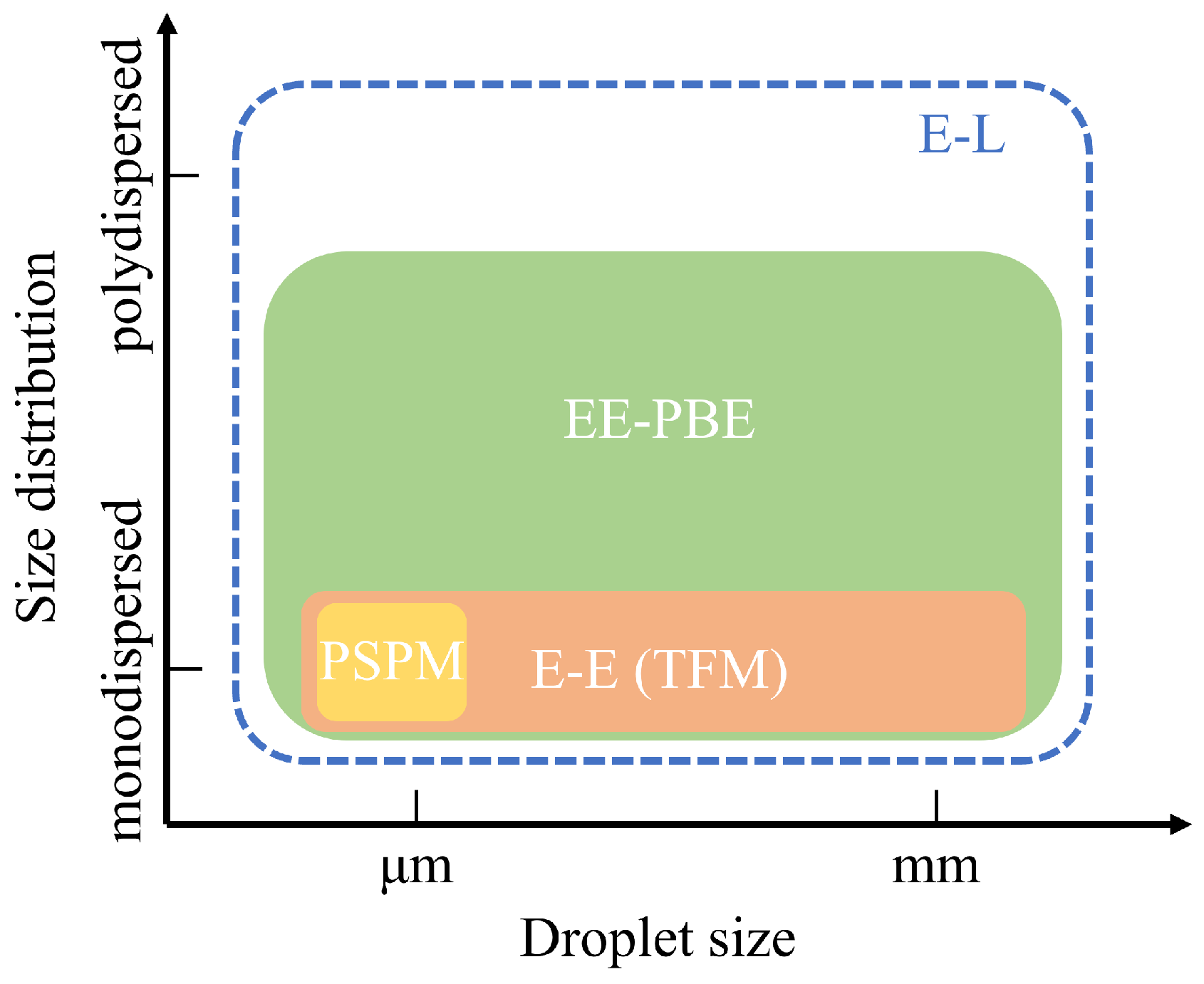
2. Methodology
2.1. Pseudo-Single-Phase Model
2.2. Two-Fluid Model
2.3. Population Balance Equation
2.4. Eulerian–Lagrangian Approach
2.5. Implementation of the Numerical Methods
3. Analysis of the Test Cases and Results
3.1. The Pseudo-Single-Phase Model for Tracer Gas
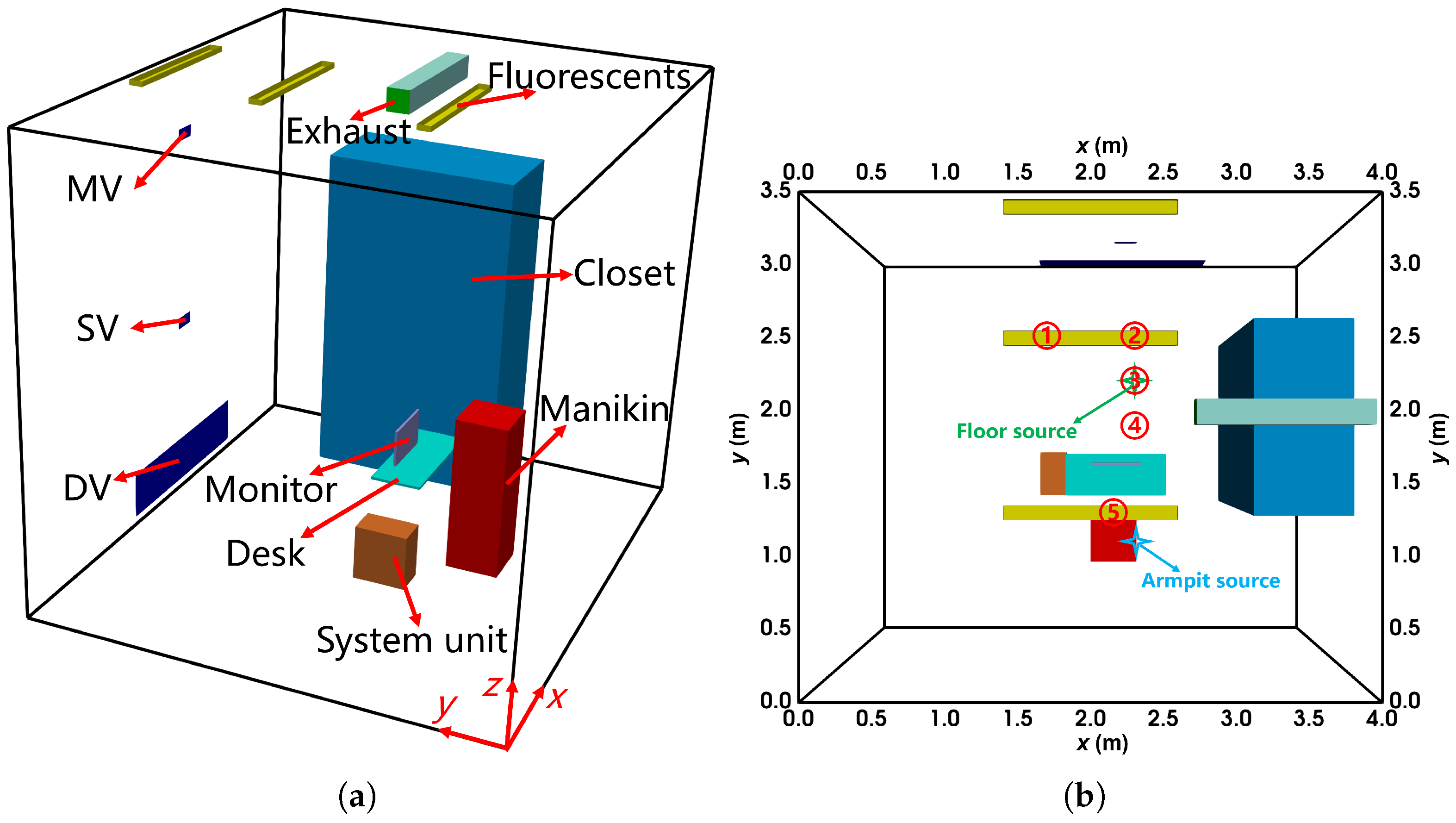
3.1.1. Case Description and Numerical Method
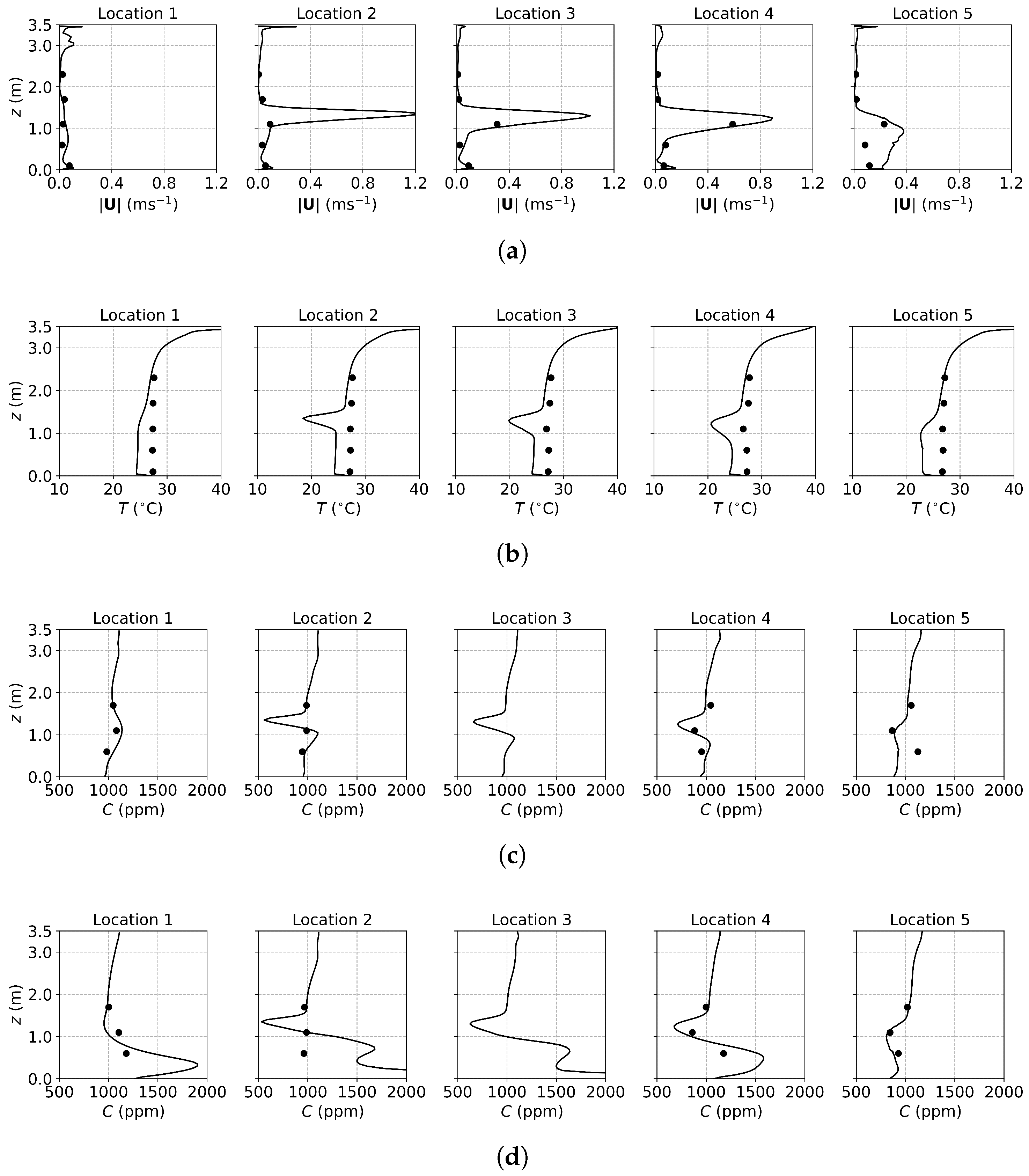
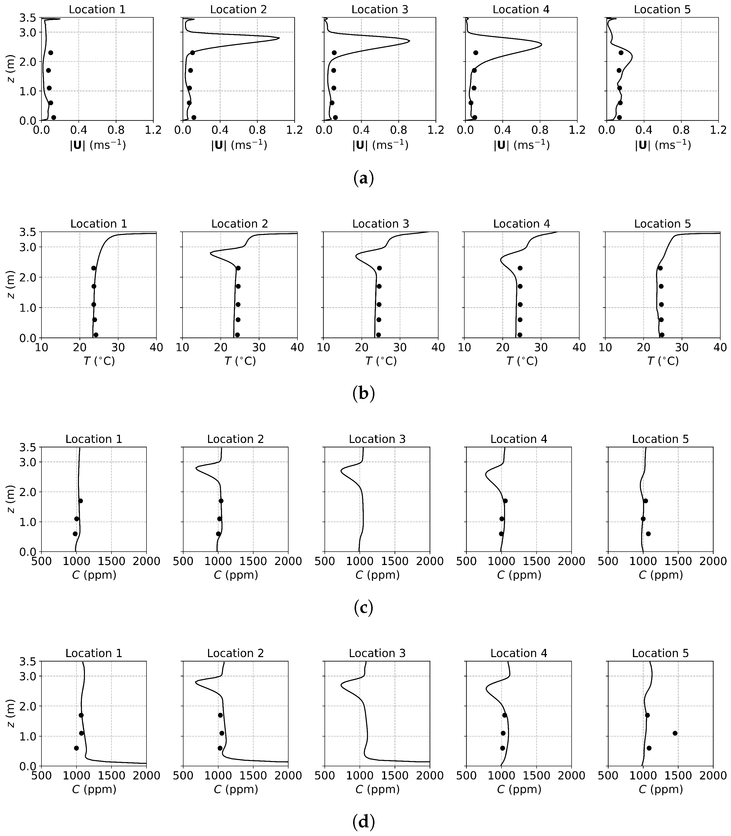
3.1.2. Results and Discussion of Tracer Gas
3.2. The Two-Fluid Model for Particles
3.2.1. Case Description and Numerical Method
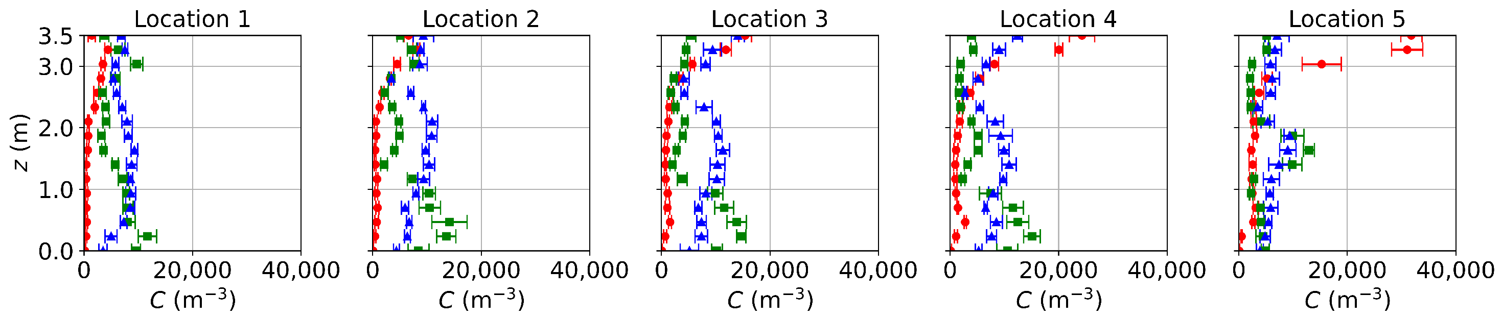
3.2.2. Results and Discussion of Non-Evaporating Particles
3.3. The TFM-PBE Coupled Approach for Evaporating Droplets
3.3.1. Case Description and Numerical Method
3.3.2. Results and Discussion of Evaporating Droplets
4. Conclusions
Supplementary Materials
Author Contributions
Funding
Data Availability Statement
Acknowledgments
Conflicts of Interest
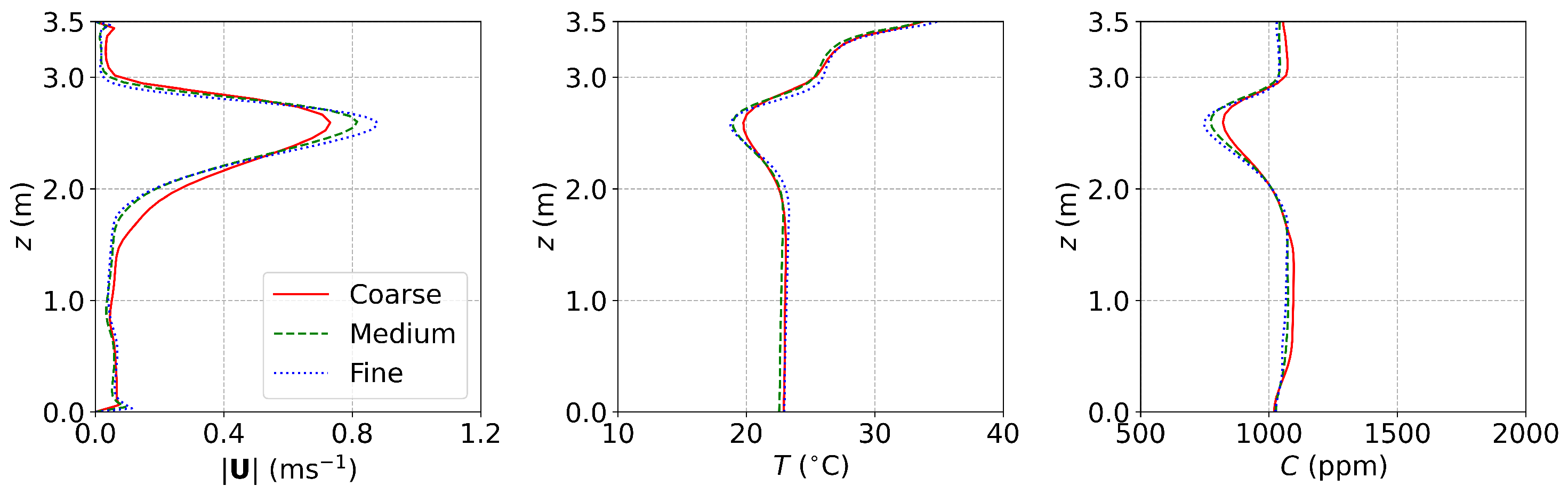
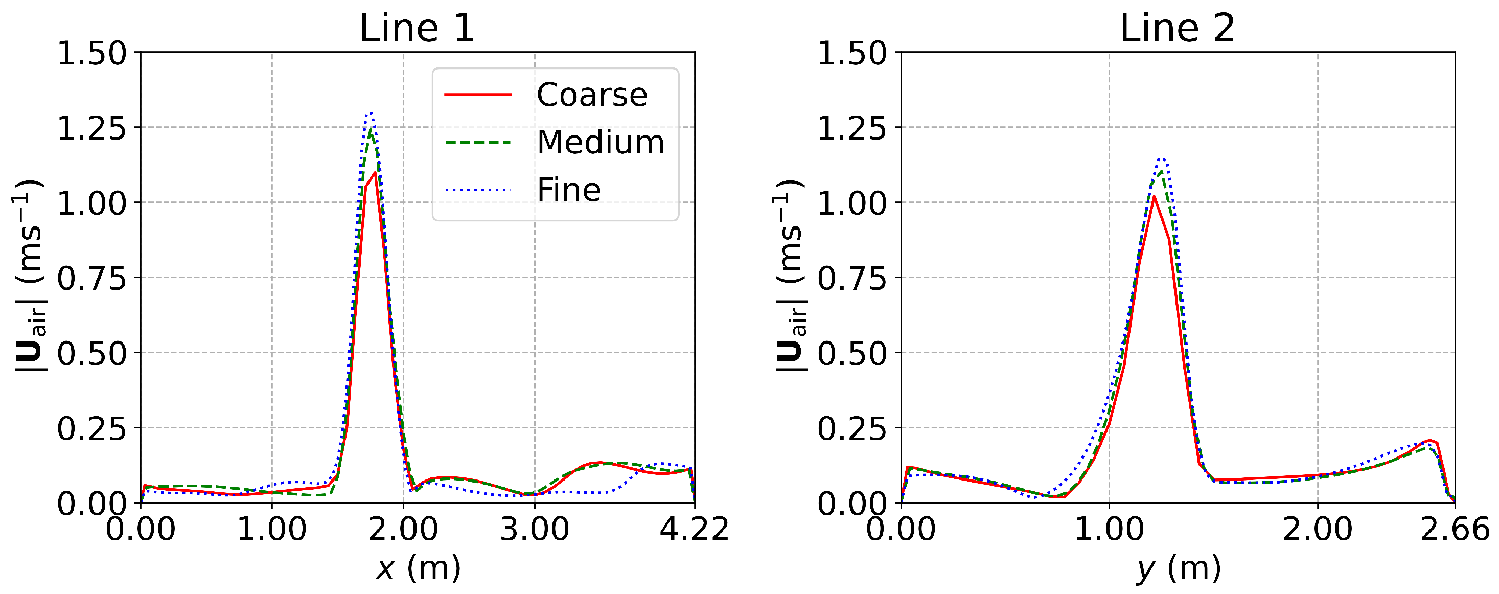
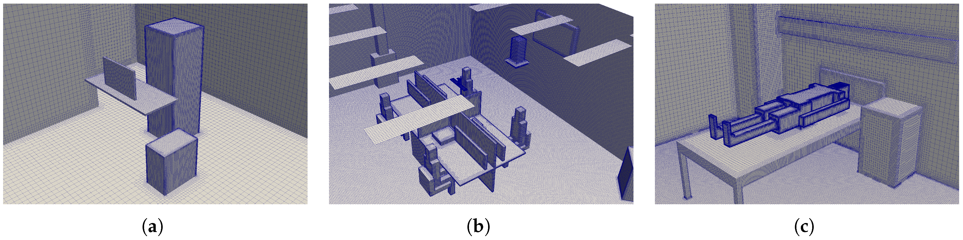
Appendix A. Grid Convergence Examination
Appendix A.1. The Office with DV, SV and MV
Appendix A.2. The Office with DV and MV

Appendix A.3. The Negative-Pressure Isolation Ward
Appendix B. Boundary Conditions

| Ventilations | Variables | Inlet | Exhaust | Walls and Surfaces | ||||
|---|---|---|---|---|---|---|---|---|
| Manikin | Floor | Fluorescents | System Unit | Others | ||||
| DV | 0.16 ms−1 1, fixedValue | free outgoing, zeroGradient | no-slip, noSlip | |||||
| T | 12.6 °C, fixedValue | free outgoing, zeroGradient | 100 W, eWHFT 2 | 23.0 °C, fixedValue | 72 W, eWHFT | 180 W, eWHFT | adiabatic, zeroGradient | |
| incoming, fixedFluxPressure | 101,325 Pa, fixedValue | no outflow, fixedFluxPressure | ||||||
| k | 9.6 × m2s−2, fixedValue | free outgoing, zeroGradient | wall function, kqRWallFunction | |||||
| 7.0 × m2s−3, fixedValue | free outgoing, zeroGradient | wall function, epsilonWallFunction | ||||||
| calculated, calculated | free outgoing, zeroGradient | wall function, alphatWallFunction | ||||||
| calculated, calculated | free outgoing, zeroGradient | wall function, nutkWallFunction | ||||||
| SV | 2.16 ms−1 fixedValue | free outgoing, zeroGradient | no-slip, noSlip | |||||
| T | 15.5 °C, fixedValue | free outgoing, zeroGradient | 100 W, eWHFT | 27.1 °C, fixedValue | 72 W, eWHFT | 180 W, eWHFT | adiabatic, zeroGradient | |
| incoming, fixedFluxPressure | 101,325 Pa, fixedValue | no outflow, fixedFluxPressure | ||||||
| k | 1.2 × m2s−2, fixedValue | free outgoing, zeroGradient | wall function, kqRWallFunction | |||||
| 4.6 × m2s−3, fixedValue | free outgoing, zeroGradient | wall function, epsilonWallFunction | ||||||
| calculated, calculated | free outgoing, zeroGradient | wall function, alphatWallFunction | ||||||
| calculated, calculated | free outgoing, zeroGradient | wall function, nutkWallFunction | ||||||
| MV | 2.16 ms−1 fixedValue | free outgoing, zeroGradient | no-slip, noSlip | |||||
| T | 11.3 °C, fixedValue | free outgoing, zeroGradient | 100 W, eWHFT | 24.0 °C, fixedValue | 72 W, eWHFT | 180 W, eWHFT | adiabatic, zeroGradient | |
| incoming, fixedFluxPressure | 101,325 Pa, fixedValue | no outflow, fixedFluxPressure | ||||||
| k | 1.2 × m2s−2, fixedValue | free outgoing, zeroGradient | wall function, kqRWallFunction | |||||
| 4.6 m2s−3, fixedValue | free outgoing, zeroGradient | wall function, epsilonWallFunction | ||||||
| calculated, calculated | free outgoing, zeroGradient | wall function, alphatWallFunction | ||||||
| calculated, calculated | free outgoing, zeroGradient | wall function, nutkWallFunction | ||||||
| Source Locations | Cases | at Inlet | at Inlet | Source Intensity |
|---|---|---|---|---|
| armpit, (2.40 m, 0.95 m, 1.00 m) | DV-A1 | 1 | 2 | kgs−1 2 |
| SV-A1 | ||||
| MV-A1 | ||||
| floor, (2.35 m, 2.20 m, 0.00 m) | DV-F1 | kgs−1 | ||
| SV-F1 | ||||
| MV-F1 |
| Ventilations | Variables | Ventilation Inlet | Emitter Inlet | Exhaust | Walls and Surfaces 1 |
|---|---|---|---|---|---|
| DV | 1.0, fixedValue | 0.999999, fixedValue | free outgoing, zeroGradient | no deposition, zeroGradient | |
| 0.0, fixedValue | 0.000001, fixedValue | free outgoing, zeroGradient | no deposition, zeroGradient | ||
| and 2 | 1.02 ms−1 fixedValue | 1.58 ms−1, fixedValue | free outgoing, zeroGradient | no-slip, noSlip | |
| incoming, fixedFluxPressure | incoming, fixedFluxPressure | 101,325 Pa, fixedValue | no outflow, fixedFluxPressure | ||
| m2s−2, fixedValue | m2s−2, fixedValue | free outgoing, zeroGradient | wall function, kqRWallFunction | ||
| m2s−3, fixedValue | m2s−3, fixedValue | free outgoing, zeroGradient | wall function, epsilonWallFunction | ||
| calculated, calculated | calculated, calculated | free outgoing, zeroGradient | wall function, alphatWallFunction | ||
| calculated, calculated | calculated, calculated | free outgoing, zeroGradient | wall function, nutkWallFunction | ||
| MV | 1.0, fixedValue | 0.999999, fixedValue | free outgoing, zeroGradient | no deposition, zeroGradient | |
| 0.0, fixedValue | 0.000001, fixedValue | free outgoing, zeroGradient | no deposition, zeroGradient | ||
| and | 2.74 ms−1, 3 fixedValue | 1.58 ms−1, fixedValue | free outgoing, zeroGradient | no-slip, noSlip | |
| incoming, fixedFluxPressure | incoming, fixedFluxPressure | 101,325 Pa, fixedValue | no outflow, fixedFluxPressure | ||
| 0.25 m2s−2, fixedValue | m2s−2, fixedValue | free outgoing, zeroGradient | wall function, kqRWallFunction | ||
| 2.1 m2s−3, fixedValue | m2s−3, fixedValue | free outgoing, zeroGradient | wall function, epsilonWallFunction | ||
| calculated, calculated | calculated, calculated | free outgoing, zeroGradient | wall function, alphatWallFunction | ||
| calculated, calculated | calculated, calculated | free outgoing, zeroGradient | wall function, nutkWallFunction |
| Boundaries | DV | MV |
|---|---|---|
| Ventilation inlet | °C, fixedValue | °C 1, fixedValue |
| Emitter inlet 2 | °C, fixedValue | °C, fixedValue |
| Fluorescents 3 | °C, fixedValue | °C, fixedValue |
| Manikin 4 | °C, fixedValue | °C, fixedValue |
| TV 4 | °C, fixedValue | °C, fixedValue |
| Computer 4 | °C, fixedValue | °C, fixedValue |
| Monitor 4 | °C, fixedValue | °C, fixedValue |
| Floor ( m) 4 | °C, fixedValue | °C, fixedValue |
| Left-hand wall ( m) 4 | °C, fixedValue | °C, fixedValue |
| Right-hand wall ( m) 4 | °C, fixedValue | °C, fixedValue |
| Front wall ( m) 4 | °C, fixedValue | °C, fixedValue |
| Back wall ( m) 4 | °C, fixedValue | °C, fixedValue |
| Back wall ( m) 4 | °C, fixedValue | °C, fixedValue |
| Ceiling ( m) 5 | °C, fixedValue | °C, fixedValue |
| Other surfaces 6 | adiabatic, zeroGradient | adiabatic, zeroGradient |
| Variables | MV Inlet | Mouth | Door Gap 1/2 | Exhaust | Manikin | Walls and Surfaces |
|---|---|---|---|---|---|---|
| 1.0, fixedValue | 0.999999, fixedValue | 1.0/1.0, fixedValue | free outgoing, zeroGradient | no deposition, zeroGradient | no deposition, zeroGradient | |
| 0.0, fixedValue | 0.000001, fixedValue | 0.0/0.0, fixedValue | free outgoing, zeroGradient | no deposition, zeroGradient | no deposition, zeroGradient | |
| and | ms−1, fixedValue | ms−1, fixedValue | / ms−1 1 fixedValue | free outgoing, zeroGradient | no-slip, noSlip | no-slip, noSlip |
| and | K, fixedValue | K, fixedValue | / K, fixedValue | free outgoing, zeroGradient | K, fixedValue | adiabatic, zeroGradient |
| incoming, fixedFluxPressure | incoming, fixedFluxPressure | incoming, fixedFluxPressure | 101,325 Pa, fixedValue | no outflow, fixedFluxPressure | no outflow, fixedFluxPressure | |
| m2s−2, fixedValue | m2s−2, fixedValue | 0.015/0.020 m2s−2, fixedValue | free outgoing, zeroGradient | wall function, kqRWallFunction | wall function, kqRWallFunction | |
| m2s−3, fixedValue | m2s−3, fixedValue | 0.11/0.17 m2s−3, fixedValue | free outgoing, zeroGradient | wall function, epsilonWallFunction | wall function, epsilonWallFunction | |
| calculated, calculated | calculated, calculated | calculated, calculated | free outgoing, zeroGradient | wall function, alphatWallFunction | wall function, alphatWallFunction | |
| calculated, calculated | calculated, calculated | calculated, calculated | free outgoing, zeroGradient | wall function, nutkWallFunction | wall function, nutkWallFunction | |
| 0.0, fixedValue | Table 3, fixedValue | 0.0/0.0, fixedValue | free outgoing, zeroGradient | no deposition, zeroGradient | no deposition, zeroGradient | |
| 0.012, fixedValue | 0.033, fixedValue | 0.012/0.012, fixedValue | free outgoing, zeroGradient | no outflow, zeroGradient | no outflow, zeroGradient |
References
- WHO. Transmission of SARS-CoV-2: Implications for Infection Prevention Precautions; Technical Report; World Health Organization: Geneva, Switzerland, 2020. [Google Scholar]
- Klepeis, N.E.; Nelson, W.C.; Ott, W.R.; Robinson, J.P.; Tsang, A.M.; Switzer, P.; Behar, J.V.; Hern, S.C.; Engelmann, W.H. The National Human Activity Pattern Survey (NHAPS): A Resource for Assessing Exposure to Environmental Pollutants. J. Expo. Sci. Environ. Epidemiol. 2001, 11, 231–252. [Google Scholar] [CrossRef]
- Chao, C.; Wan, M.; Morawska, L.; Johnson, G.; Ristovski, Z.; Hargreaves, M.; Mengersen, K.; Corbett, S.; Li, Y.; Xie, X.; et al. Characterization of Expiration Air Jets and Droplet Size Distributions Immediately at the Mouth Opening. J. Aerosol Sci. 2009, 40, 122–133. [Google Scholar] [CrossRef] [PubMed]
- Balachandar, S.; Zaleski, S.; Soldati, A.; Ahmadi, G.; Bourouiba, L. Host-to-Host Airborne Transmission as a Multiphase Flow Problem for Science-Based Social Distance Guidelines. Int. J. Multiph. Flow 2020, 132, 103439. [Google Scholar] [CrossRef]
- Liu, J.; Duan, Y. Saliva: A Potential Media for Disease Diagnostics and Monitoring. Oral Oncol. 2012, 48, 569–577. [Google Scholar] [CrossRef]
- Hatif, I.H.; Mohamed Kamar, H.; Kamsah, N.; Wong, K.Y.; Tan, H. Influence of Office Furniture on Exposure Risk to Respiratory Infection under Mixing and Displacement Air Distribution Systems. Build. Environ. 2023, 239, 110292. [Google Scholar] [CrossRef]
- Li, X.; Shang, Y.; Yan, Y.; Yang, L.; Tu, J. Modelling of Evaporation of Cough Droplets in Inhomogeneous Humidity Fields Using the Multi-Component Eulerian-Lagrangian Approach. Build. Environ. 2018, 128, 68–76. [Google Scholar] [CrossRef]
- Tang, J.; Noakes, C.; Nielsen, P.; Eames, I.; Nicolle, A.; Li, Y.; Settles, G. Observing and Quantifying Airflows in the Infection Control of Aerosol- and Airborne-Transmitted Diseases: An Overview of Approaches. J. Hosp. Infect. 2011, 77, 213–222. [Google Scholar] [CrossRef]
- Cao, G.; Sirén, K.; Kilpeläinen, S. Modelling and Experimental Study of Performance of the Protected Occupied Zone Ventilation. Energy Build. 2014, 68, 515–531. [Google Scholar] [CrossRef]
- Olmedo, I.; Nielsen, P.V.; Ruiz de Adana, M.; Jensen, R.L.; Grzelecki, P. Distribution of Exhaled Contaminants and Personal Exposure in a Room Using Three Different Air Distribution Strategies: Distribution of Exhaled Contaminants. Indoor Air 2012, 22, 64–76. [Google Scholar] [CrossRef]
- Yang, J.; Sekhar, S.C.; Cheong, K.W.D.; Raphael, B. Performance Evaluation of a Novel Personalized Ventilation-Personalized Exhaust System for Airborne Infection Control. Indoor Air 2015, 25, 176–187. [Google Scholar] [CrossRef]
- Tung, Y.C.; Shih, Y.C.; Hu, S.C.; Chang, Y.L. Experimental Performance Investigation of Ventilation Schemes in a Private Bathroom. Build. Environ. 2010, 45, 243–251. [Google Scholar] [CrossRef]
- Lu, Y.; Oladokun, M.; Lin, Z. Reducing the Exposure Risk in Hospital Wards by Applying Stratum Ventilation System. Build. Environ. 2020, 183, 107204. [Google Scholar] [CrossRef]
- Ai, Z.; Mak, C.M.; Gao, N.; Niu, J. Tracer Gas Is a Suitable Surrogate of Exhaled Droplet Nuclei for Studying Airborne Transmission in the Built Environment. Build. Simul. 2020, 13, 489–496. [Google Scholar] [CrossRef] [PubMed]
- Bivolarova, M.; Ondráček, J.; Melikov, A.; Ždímal, V. A Comparison between Tracer Gas and Aerosol Particles Distribution Indoors: The Impact of Ventilation Rate, Interaction of Airflows, and Presence of Objects. Indoor Air 2017, 27, 1201–1212. [Google Scholar] [CrossRef] [PubMed]
- Rivas, E.; Santiago, J.L.; Martín, F.; Martilli, A. Impact of Natural Ventilation on Exposure to SARS-CoV-2 in Indoor/Semi-Indoor Terraces Using CO2 Concentrations as a Proxy. J. Build. Eng. 2022, 46, 103725. [Google Scholar] [CrossRef]
- Tian, X.; Li, B.; Ma, Y.; Liu, D.; Li, Y.; Cheng, Y. Experimental Study of Local Thermal Comfort and Ventilation Performance for Mixing, Displacement and Stratum Ventilation in an Office. Sustain. Cities Soc. 2019, 50, 101630. [Google Scholar] [CrossRef]
- Ameen, A.; Cehlin, M.; Larsson, U.; Karimipanah, T. Experimental Investigation of the Ventilation Performance of Different Air Distribution Systems in an Office Environment—Cooling Mode. Energies 2019, 12, 1354. [Google Scholar] [CrossRef]
- Kong, X.; Chang, Y.; Fan, M.; Li, H. Analysis on the Thermal Performance of Low-Temperature Radiant Floor Coupled with Intermittent Stratum Ventilation (LTR-ISV) for Space Heating. Energy Build. 2023, 278, 112623. [Google Scholar] [CrossRef]
- Kong, X.; Wang, Z.; Fan, M.; Li, H. Analysis on the Energy Efficiency, Thermal Performance and Infection Intervention Characteristics of Interactive Cascade Ventilation (ICV). J. Build. Eng. 2023, 68, 106045. [Google Scholar] [CrossRef]
- Zhou, Y.; Ji, S. Experimental and Numerical Study on the Transport of Droplet Aerosols Generated by Occupants in a Fever Clinic. Build. Environ. 2021, 187, 107402. [Google Scholar] [CrossRef]
- Liu, S.; Koupriyanov, M.; Paskaruk, D.; Fediuk, G.; Chen, Q. Investigation of Airborne Particle Exposure in an Office with Mixing and Displacement Ventilation. Sustain. Cities Soc. 2022, 79, 103718. [Google Scholar] [CrossRef] [PubMed]
- Zhuang, X.; Xu, Y.; Zhang, L.; Li, X.; Lu, J. Experiment and Numerical Investigation of Inhalable Particles and Indoor Environment with Ventilation System. Energy Build. 2022, 271, 112309. [Google Scholar] [CrossRef] [PubMed]
- Xu, J.; Guo, H.; Zhang, Y.; Lyu, X. Effectiveness of Personalized Air Curtain in Reducing Exposure to Airborne Cough Droplets. Build. Environ. 2022, 208, 108586. [Google Scholar] [CrossRef]
- Wang, Y.; Liu, Z.; Liu, H.; Wu, M.; He, J.; Cao, G. Droplet Aerosols Transportation and Deposition for Three Respiratory Behaviors in a Typical Negative Pressure Isolation Ward. Build. Environ. 2022, 219, 109247. [Google Scholar] [CrossRef]
- Na, H.; Kim, H.; Kim, T. Dispersion of Droplets Due to the Use of Air Purifiers during Summer: Focus on the Spread of COVID-19. Build. Environ. 2023, 234, 110136. [Google Scholar] [CrossRef]
- Zhong, K.; Yang, X.; Kang, Y. Effects of Ventilation Strategies and Source Locations on Indoor Particle Deposition. Build. Environ. 2010, 45, 655–662. [Google Scholar] [CrossRef]
- Makhoul, A.; Ghali, K.; Ghaddar, N.; Chakroun, W. Investigation of Particle Transport in Offices Equipped with Ceiling-Mounted Personalized Ventilators. Build. Environ. 2013, 63, 97–107. [Google Scholar] [CrossRef]
- Li, T.; Essah, E.A.; Wu, Y.; Cheng, Y.; Liao, C. Numerical Comparison of Exhaled Particle Dispersion under Different Air Distributions for Winter Heating. Sustain. Cities Soc. 2023, 89, 104342. [Google Scholar] [CrossRef]
- Huang, X.; Saha, S.C.; Saha, G.; Francis, I.; Luo, Z. Transport and Deposition of Microplastics and Nanoplastics in the Human Respiratory Tract. Environ. Adv. 2024, 16, 100525. [Google Scholar] [CrossRef]
- Talaat, M.; Si, X.; Xi, J. Evaporation Dynamics and Dosimetry Methods in Numerically Assessing MDI Performance in Pulmonary Drug Delivery. Fluids 2024, 9, 286. [Google Scholar] [CrossRef]
- Huang, X.; Yin, Y.; Saha, G.; Francis, I.; Saha, S.C. A Comprehensive Numerical Study on the Transport and Deposition of Nasal Sprayed Pharmaceutical Aerosols in a Nasal-To-Lung Respiratory Tract Model. Part. Part. Syst. Charact. 2025, 42, 2400004. [Google Scholar] [CrossRef]
- Wang, L.; Dai, X.; Wei, J.; Ai, Z.; Fan, Y.; Tang, L.; Jin, T.; Ge, J. Numerical Comparison of the Efficiency of Mixing Ventilation and Impinging Jet Ventilation for Exhaled Particle Removal in a Model Intensive Care Unit. Build. Environ. 2021, 200, 107955. [Google Scholar] [CrossRef]
- Ren, J.; Wang, Y.; Liu, Q.; Liu, Y. Numerical Study of Three Ventilation Strategies in a Prefabricated COVID-19 Inpatient Ward. Build. Environ. 2021, 188, 107467. [Google Scholar] [CrossRef]
- Liu, S.; Deng, Z. Transmission and Infection Risk of COVID-19 When People Coughing in an Elevator. Build. Environ. 2023, 238, 110343. [Google Scholar] [CrossRef] [PubMed]
- Borro, L.; Mazzei, L.; Raponi, M.; Piscitelli, P.; Miani, A.; Secinaro, A. The Role of Air Conditioning in the Diffusion of Sars-CoV-2 in Indoor Environments: A First Computational Fluid Dynamic Model, Based on Investigations Performed at the Vatican State Children’s Hospital. Environ. Res. 2021, 193, 110343. [Google Scholar] [CrossRef] [PubMed]
- Li, X.; Feng, B. Transmission of Droplet Aerosols in an Elevator Cabin: Effect of the Ventilation Mode. Build. Environ. 2023, 236, 110261. [Google Scholar] [CrossRef]
- Lu, Y.; Lin, Z. Coughed Droplet Dispersion Pattern in Hospital Ward under Stratum Ventilation. Build. Environ. 2022, 208, 108602. [Google Scholar] [CrossRef]
- Zhang, Y.; Feng, G.; Bi, Y.; Cai, Y.; Zhang, Z.; Cao, G. Distribution of Droplet Aerosols Generated by Mouth Coughing and Nose Breathing in an Air-Conditioned Room. Sustain. Cities Soc. 2019, 51, 101721. [Google Scholar] [CrossRef]
- Bensaid, S.; Marchisio, D.; Fino, D.; Saracco, G.; Specchia, V. Modelling of Diesel Particulate Filtration in Wall-Flow Traps. Chem. Eng. J. 2009, 154, 211–218. [Google Scholar] [CrossRef]
- Wang, F.; Zhang, T.T.; You, R.; Chen, Q. Evaluation of Infection Probability of Covid-19 in Different Types of Airliner Cabins. Build. Environ. 2023, 234, 110159. [Google Scholar] [CrossRef]
- Park, S.; Mistrick, R.; Rim, D. Performance of Upper-Room Ultraviolet Germicidal Irradiation (UVGI) System in Learning Environments: Effects of Ventilation Rate, UV Fluence Rate, and UV Radiating Volume. Sustain. Cities Soc. 2022, 85, 104048. [Google Scholar] [CrossRef]
- Shao, X.; Wen, X.; Paek, R.; Liu, Y.; Jian, Y.; Liu, W. Use of Recirculated Air Curtains inside Ventilated Rooms for the Isolation of Transient Contaminant. Energy Build. 2022, 273, 112407. [Google Scholar] [CrossRef]
- Ren, C.; Xi, C.; Wang, J.; Feng, Z.; Nasiri, F.; Cao, S.J.; Haghighat, F. Mitigating COVID-19 Infection Disease Transmission in Indoor Environment Using Physical Barriers. Sustain. Cities Soc. 2021, 74, 103175. [Google Scholar] [CrossRef]
- Ren, C.; Zhu, H.C.; Cao, S.J. Ventilation Strategies for Mitigation of Infection Disease Transmission in an Indoor Environment: A Case Study in Office. Buildings 2022, 12, 180. [Google Scholar] [CrossRef]
- D’Alicandro, A.C.; Mauro, A. Effects of Operating Room Layout and Ventilation System on Ultrafine Particle Transport and Deposition. Atmos. Environ. 2022, 270, 118901. [Google Scholar] [CrossRef]
- Yan, Y.; Li, X.; Ito, K. Numerical Investigation of Indoor Particulate Contaminant Transport Using the Eulerian-Eulerian and Eulerian-Lagrangian Two-Phase Flow Models. Exp. Comput. Multiph. Flow 2020, 2, 31–40. [Google Scholar] [CrossRef]
- Pei, G.; Taylor, M.; Rim, D. Human Exposure to Respiratory Aerosols in a Ventilated Room: Effects of Ventilation Condition, Emission Mode, and Social Distancing. Sustain. Cities Soc. 2021, 73, 103090. [Google Scholar] [CrossRef]
- Zhao, B.; Yang, C.; Yang, X.; Liu, S. Particle Dispersion and Deposition in Ventilated Rooms: Testing and Evaluation of Different Eulerian and Lagrangian Models. Build. Environ. 2008, 43, 388–397. [Google Scholar] [CrossRef]
- Chen, F.; Yu, S.C.; Lai, A.C. Modeling Particle Distribution and Deposition in Indoor Environments with a New Drift–Flux Model. Atmos. Environ. 2006, 40, 357–367. [Google Scholar] [CrossRef]
- D’Alicandro, A.C.; Mauro, A. Air Change per Hour and Inlet Area: Effects on Ultrafine Particle Concentration and Thermal Comfort in an Operating Room. J. Aerosol Sci. 2023, 171, 106183. [Google Scholar] [CrossRef]
- Feng, Y.; Li, D.; Marchisio, D.; Vanni, M.; Buffo, A. A Computational Fluid Dynamics—Population Balance Equation Approach for Evaporating Cough Droplets Transport. Int. J. Multiph. Flow 2023, 165, 104500. [Google Scholar] [CrossRef]
- Crowe, C.T.; Schwarzkopf, J.D.; Sommerfeld, M.; Tsuji, Y. Multiphase Flows with Droplets and Particles, 2nd ed.; CRC Press: Boca Raton, FL, USA, 2012. [Google Scholar] [CrossRef]
- Marchisio, D.L.; Fox, R.O. Computational Models for Polydisperse Particulate and Multiphase Systems; Cambridge Series in Chemical Engineering; Cambridge University Press: Cambridge, MA, USA, 2013. [Google Scholar] [CrossRef]
- Balachandar, S.; Eaton, J.K. Turbulent Dispersed Multiphase Flow. Annu. Rev. Fluid Mech. 2010, 42, 111–133. [Google Scholar] [CrossRef]
- Subramaniam, S. Lagrangian–Eulerian Methods for Multiphase Flows. Prog. Energy Combust. Sci. 2013, 39, 215–245. [Google Scholar] [CrossRef]
- Capecelatro, J.; Desjardins, O. An Euler–Lagrange Strategy for Simulating Particle-Laden Flows. J. Comput. Phys. 2013, 238, 1–31. [Google Scholar] [CrossRef]
- Biswas, R.; Pal, A.; Pal, R.; Sarkar, S.; Mukhopadhyay, A. Risk Assessment of COVID Infection by Respiratory Droplets from Cough for Various Ventilation Scenarios inside an Elevator: An OpenFOAM-Based Computational Fluid Dynamics Analysis. Phys. Fluids 2022, 34, 013318. [Google Scholar] [CrossRef] [PubMed]
- ESI-OpenCFD. ESI OpenCFD Release OpenFOAM® V2106. 2021. Available online: https://www.openfoam.com/news/main-news/openfoam-v2106 (accessed on 9 July 2025).
- Zhang, T.T.; Lee, K.; Chen, Q.Y. A Simplified Approach to Describe Complex Diffusers in Displacement Ventilation for CFD Simulations. Indoor Air 2009, 19, 255–267. [Google Scholar] [CrossRef]
- King, M.F.; Noakes, C.J.; Sleigh, P.A. Modeling Environmental Contamination in Hospital Single- and Four-Bed Rooms. Indoor Air 2015, 25, 694–707. [Google Scholar] [CrossRef]
- Yakhot, V.; Orszag, S.A.; Thangam, S.; Gatski, T.B.; Speziale, C.G. Development of Turbulence Models for Shear Flows by a Double Expansion Technique. Phys. Fluids A Fluid Dyn. 1992, 4, 1510–1520. [Google Scholar] [CrossRef]
- Yuce, B.E.; Pulat, E. Forced, Natural and Mixed Convection Benchmark Studies for Indoor Thermal Environments. Int. Commun. Heat Mass Transf. 2018, 92, 1–14. [Google Scholar] [CrossRef]
- D’Alicandro, A.C.; Mauro, A. Experimental and Numerical Analysis of CO2 Transport inside a University Classroom: Effects of Turbulent Models. J. Build. Perform. Simul. 2023, 16, 434–459. [Google Scholar] [CrossRef]
- Cheng, Y.; Lin, Z. Experimental Study of Airflow Characteristics of Stratum Ventilation in a Multi-Occupant Room with Comparison to Mixing Ventilation and Displacement Ventilation. Indoor Air 2015, 25, 662–671. [Google Scholar] [CrossRef] [PubMed]
- Zhang, Z.; Chen, Q. Experimental Measurements and Numerical Simulations of Particle Transport and Distribution in Ventilated Rooms. Atmos. Environ. 2006, 40, 3396–3408. [Google Scholar] [CrossRef]


| Variables | DV | MV |
|---|---|---|
| Total particle number (-) | 1,000,000 | 1,000,000 |
| Active particle number (-) 1 | 759,987 | 877,232 |
| Maximum particle velocity () | 1.57 | 2.36 |
| Average particle velocity () | 0.15 | 0.13 |
| Particle number for (-) 2 | 212,791 | 107,010 |
| Average age of active particles (s) | 221.32 | 235.75 |
| Approach | DV (h) | MV (h) |
|---|---|---|
| PSPM | 0.51 | 0.65 |
| TFM | 1.36 | 1.64 |
| E-L | 1.86 | 1.80 |
| (-) | () | () | () | (-) |
|---|---|---|---|---|
Disclaimer/Publisher’s Note: The statements, opinions and data contained in all publications are solely those of the individual author(s) and contributor(s) and not of MDPI and/or the editor(s). MDPI and/or the editor(s) disclaim responsibility for any injury to people or property resulting from any ideas, methods, instructions or products referred to in the content. |
© 2025 by the authors. Licensee MDPI, Basel, Switzerland. This article is an open access article distributed under the terms and conditions of the Creative Commons Attribution (CC BY) license (https://creativecommons.org/licenses/by/4.0/).
Share and Cite
Feng, Y.; Li, D.; Marchisio, D.; Vanni, M.; Buffo, A. Indoor Transmission of Respiratory Droplets Under Different Ventilation Systems Using the Eulerian Approach for the Dispersed Phase. Fluids 2025, 10, 185. https://doi.org/10.3390/fluids10070185
Feng Y, Li D, Marchisio D, Vanni M, Buffo A. Indoor Transmission of Respiratory Droplets Under Different Ventilation Systems Using the Eulerian Approach for the Dispersed Phase. Fluids. 2025; 10(7):185. https://doi.org/10.3390/fluids10070185
Chicago/Turabian StyleFeng, Yi, Dongyue Li, Daniele Marchisio, Marco Vanni, and Antonio Buffo. 2025. "Indoor Transmission of Respiratory Droplets Under Different Ventilation Systems Using the Eulerian Approach for the Dispersed Phase" Fluids 10, no. 7: 185. https://doi.org/10.3390/fluids10070185
APA StyleFeng, Y., Li, D., Marchisio, D., Vanni, M., & Buffo, A. (2025). Indoor Transmission of Respiratory Droplets Under Different Ventilation Systems Using the Eulerian Approach for the Dispersed Phase. Fluids, 10(7), 185. https://doi.org/10.3390/fluids10070185