Abstract
This paper considers the problem of estimating the quantitative parameters of a two-phase fluid flow in a well based on the dynamic physical flow model. This is a challenging problem in the oil and gas industry, where the knowledge of multiphase production rates plays an important role during reservoir characterization, production optimization and reservoir management. As the direct measurement of these rates is not easily available, they can be inferred from conventional sensors (e.g., pressure gauges) in combination with a dynamic multiphase flow model. The methodology proposed in this work uses inverse modeling concepts to estimate flow rates that are not measured directly. The mismatch between the available data and model prediction is numerically minimized, leading to the optimal set of dynamic flow variables characterizing the flow. Two different scenarios are considered: firstly, when the well has only a flow meter located at the wellhead (minimum amount of available information), and when the well has distributed pressure sensors in addition to the topside flow meter (maximum amount of information). The feasibility of the proposed concept is assessed via several simulation-based case studies.
1. Introduction
Nowadays, the requirements for hydrocarbon production include not only short-term economic considerations, but also the need to comply with strategic goals, which include increasing the oil recovery factor while maintaining sustainability constraints [1]. To achieve these goals, long-term planning with intelligent oilfield management strategies is often employed [2]. These strategies, in turn, require significant amounts of reliable and up-to-date information obtained from the reservoir. In particular, the measurement of multiphase production rates provides indispensable knowledge for production monitoring and reservoir optimization and characterization [3,4].
The most commonly used approach to measure the production rates is by multiphase flow meters or test separators, which have an extensively demonstrated track record of application in the oil and gas industry [5]. Unfortunately, multiphase flow meters are expensive and accurate only within a limited operating range. More importantly, these devices are installed at the wellhead and hence do not provide information either about downhole inflow rates or about spatial flow and composition distribution. As an alternative, the most complete picture of the phenomena can be deduced from the results of geophysical logging, which allow the estimation of the inflow profile in the entire wellbore [6]. However, in practice, this approach may have a rather low accuracy due to the difficulties in unambiguously determining the composition of the multiphase fluid at each measured depth location. Additionally, logging as such is a technologically challenging operation, especially for openhole long horizontal wells with intelligent completions. An overview of these challenges is available in [7].
As an alternative to the direct instrumental measurement of multiphase flow rates, a soft metering approach (or soft-sensing) can be used [8]. This is based on the idea of utilizing the data from conventional cheap sensors, such as pressure and temperature gauges, which are more commonly used as a part of wellbore instrumentation. All these available data are then used to infer the unknown multiphase rates through some kind of predictive model, which can be classified as data-driven or physics-based [9]. In the data-driven approach, no background information on multiphase flow physics is needed. Instead, an implicit relationship is formulated which relates the available measurements and target flow rates. There are multiple examples where machine learning and data analytics methods have been used as the predictors for multiphase production technology [10,11,12,13]. This can be considered a black box method, where the embedded dynamics are introduced through the analysis of input and output data, rather than describing them by any conservation laws. Consequently, the data-driven approach is missing generality and demonstrates poor performance over a long horizon of prediction.
Alternatively, the dynamic behavior of multiphase wellbore flow can be described by a mathematical model. Such models are established based on known conservation laws of mass, momentum and energy, which are supplemented by a number of empirical relationships. These empirical closures are the main source of uncertainty for the physics-driven approach. Additionally, any multiphase flow model predicts the flow rates based on the known inputs (such as the boundary conditions and inflow from the reservoir). However, often, these variables are actually the target of the estimation process, and hence the direct modeling approach may fail. This challenge can be mitigated by implementing a hybrid approach, where the measurements from the sensors and the data are combined in an intelligent way, which aims to eliminate the disadvantages of both strategies and capitalize on the strong parts. Some known examples of such hybridization include grey-box modeling [14], where a feed-forward neural network is combined with a mechanistic model of the hydrocarbon production system. In [15], several phenomenological flow models have been calibrated with well pressure and temperature data through data reconciliation. A hybrid modeling approach, where physics-based transient multiphase flow simulations are combined with machine learning, has been introduced in [16]. Several methods to incorporate first principles physical models into the machine learning algorithms for multiphase flow rate estimation are discussed in [17]. From the virtual flow metering perspective, the hybrid method can be seen as an inverse problem solution, where the available sensor data is used to adjust the multiphase rates through the application of a model-based approach. Then, the mismatch between the simulated and measured data is minimized, leading to the set of optimal inflow rates. In a similar way, the parameters of a multiphase flow model can be refined, as has been demonstrated in [18].
If such a flow model is available, then the inflow assessment becomes a purely technical problem. In particular, in the framework of the current work, the drift–flux model [19,20] is considered for simulating the transport of a two-phase oil–gas mixture. To solve the soft-sensing problem, the Kalman filter [21] and its various non-linear variations are often used. Thus, in [22], inflow estimation based on well pressure data was performed, and in [23,24], similar techniques were successfully applied to the case of gas lift wells. In addition, in [25], it was shown that inflow estimation methods based on the use of the Kalman filter have a number of advantages over methods that involve minimizing the residual, composed of the discrepancy between the predicted sensor readings and their actual values [26]. However, it is necessary to highlight some obvious disadvantages of the Kalman filter, namely, the very high complexity of constructing the filter itself in each individual case (especially given that some of the equations of the flow model are specified implicitly), as well as its fundamentally recursive nature, due to which a number of restrictions appear on the sets of measured data fed to the input of the computational algorithm. In addition, a significant limitation when using the Kalman filter is supplementing any additional conditions that the flow parameters must satisfy. In this regard, in this paper, an approach to inflow estimation based on numerical optimization of the residual is developed, but under the assumption that some flow variables are defined by a piecewise constant function of time (which can occur, for example, in the case when the value of the wellbore production is regulated through some external control). As will be demonstrated in further sections, such an assumption is quite sufficient for the specified technique to ensure the receipt of quite reliable inflow estimates even under the condition of noisy input data corresponding to direct measurements using sensors in the well. In addition, as the number of sensors available in a well is generally limited, the sensitivity to measurement availability becomes important. While the current work focuses on the application of downhole pressure measurements, the inflow from the reservoir to the well could be estimated using temperature gauges. Alternatively, fiber optic temperature sensors are widely employed to measure continuous temperature profiles along the wellbore. Distributed temperature measurements are especially important for wells with several production and injection intervals, as they can provide valuable information on real-time inflow profiling, which has been performed by the ensemble Kalman filter in [27]. Other examples of using well temperature distribution to estimate the wellbore flow rates are given in [28,29].
This paper is organized as follows. First, the problem of inflow estimation to an arbitrary inclined well is introduced. Then, the physical flow model is presented with an approach to the numerical solution. This is followed by a series of computational examples, which illustrate the feasibility of the proposed approach. The challenge of measurement availability is also addressed in the current work, where scenarios with different sets of available data are considered. The paper ends with the conclusions and recommendations for future work.
2. Formulation of the Estimation Problem
The widely adopted technique for multiphase flow modeling in wellbores and pipelines is by using the approximate one-dimensional approach, which is supported by a substantial length-to-diameter aspect ratio. This formulation is obtained from averaging three-dimensional Navier–Stokes equations under the assumption that the flow is convection-dominated. The diffusion terms are replaced by empirical relationships, such as frictional pressure losses, which are dependent on the actual conditions and flow regime. The wellbore or pipeline is then discretized by the finite number of grid blocks and the system of simplified partial differential equations is solved numerically using an appropriate mathematical technique.
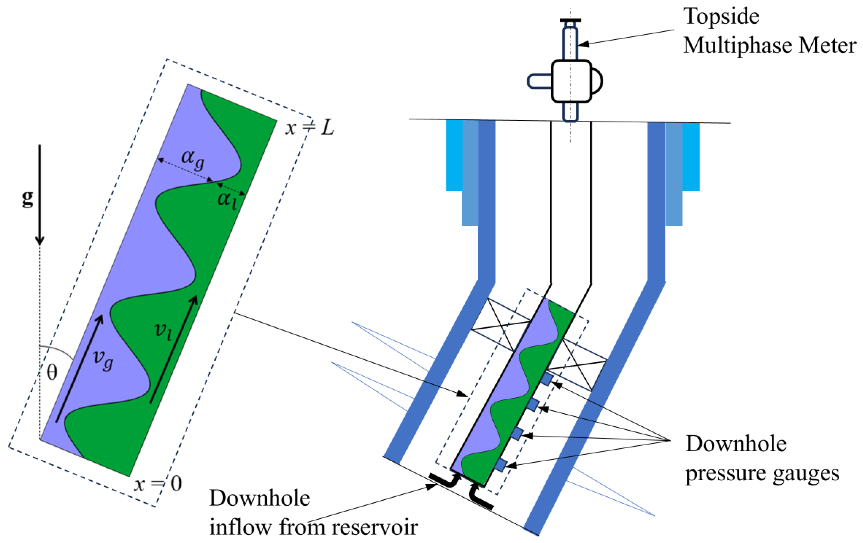
The flow of a two-phase mixture of oil and gas is considered in a deviated-from-vertical well of length L. According to the one-dimensional formulation, the flow can be described by five quantities that are functionally dependent on the time t and the coordinate x along the well axis (see Figure 1), namely, as follows: the velocities vg and vl of gas and oil, respectively, the volumetric fractions αg and αl occupied by gas and oil in the cross-sectional area of the pipe and the pressure P. The details of the physical model used are presented in Section 2.
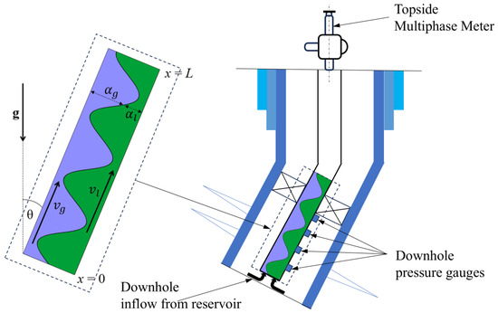
Figure 1.
Schematic representation of a producing well equipped with various sensors. Oil and gas are shown in green and blue, respectively.
Additionally, the specific mass flow rates of individual phases are introduced (per unit of well cross-sectional area), which are defined as follows: Qg(x, t) = αgρgvg for gas and Ql(x, t) = αlρlvl for oil (here, ρg and ρl are the densities of gas and oil, respectively). The values Qg(x = L, t) and Ql(x = L, t) represent the mass flow rates of the phases at the wellhead, and it is assumed that they can be measured at each time t using a topside flow meter located at the wellhead. In addition, several pressure gauges (as indicated in Figure 1) are installed in the well, providing the readings of pressure P(x, t) at several locations downhole. Two distinct scenarios are introduced: firstly, when the well has only a topside flow meter, and secondly, when the well has both a flow meter and pressure sensors. The problem can be formulated as follows: based on the measurements available within a given scenario, it is necessary to estimate the inflow at x = 0 for an arbitrary moment of time t. Thus, the estimation problem can be described by the following statement:
Minimum data (flowmeter only): Qg,l(x = L, t) → Qg,l(x = 0, t)
Maximum data (flowmeter and pressure gauges): Qg,l(x = L, t), P(x, t) → Qg,l(x = 0, t)
Note that from a mathematical point of view, the scenario with maximum information available contains redundancy, since the functions Qg,l(x = L, t) and P(x, t) are not completely independent, and in the presence of a fixed hydrodynamic flow model, the measured values of the pressure and flow rates at the wellhead can impose certain restrictions on each other or even be partially expressed through each other. However, in practice, the results of such measurements will contain various kinds of uncertainties, including the influence of noise, as a result of which the use of an excessive amount of input information not only does not lead to contradictions, but also ensures greater stability of the calculation algorithms in the presence of random errors in the measured data.
In this work, the scenarios where the inflow is represented by a piecewise constant function are considered. This assumption originates from the idea that significant changes in fluid flow rates entering the well are associated with some external control, namely with the manipulation of the topside choke. It is the certain choke opening set over a period of hydrocarbon production, which is used to maintain the wellhead pressure. Variations in the wellhead pressure P(x = L, t) would consequently lead to the changes in downhole pressure P(x = 0, t), which is in direct link to the inflow production rates Qg,l(x = 0, t) through the productivity index relationship, which is the measure of the wellbore productivity potential evaluated at pseudo-state conditions. Alternatively, the inflow from the reservoir to the wellbore can be specified directly as a predefined piecewise constant function. The latter case corresponds to the scenarios where inflow distribution is driven by changes in the reservoir pressure through the production phases of the reservoir.
It should be emphasized that the piecewise constant type of the flow parameters over time is not a necessary condition for the applicability of the techniques presented in this work. The developed methodology can be applied in cases where the corresponding functions are a priori considered piecewise linear or are represented by low-degree polynomials. Such constraints help to reduce the problem of identifying the functional dependence of a flow parameter on time with a small set of numerical values. The fewer values that are included in this target set, the more effectively arbitrary problems of numerical optimization aimed at finding these values will be solved. This is the main driving factor which determines the choice of the simplest form for the inflow relationship. For example, selecting piecewise constant approximation over piecewise linear decreases the number of parameters to be estimated by factor of two, which in turn increases the computational speed by an order of magnitude. Nevertheless, even in the absence of reliable a priori information about the type of inflow relationship, it can, of course, be approximately specified by a set of numerical values corresponding to the arbitrary time-series. Therefore, the presented methods remain theoretically applicable even for generic time-series, although in practice the use of optimization approaches may prove meaningless due to excessive computational costs.
3. Physical and Numerical Model of Multiphase Flow
3.1. Hydrodynamics of Two-Phase Flow
Within the one-dimensional approach for flow modeling, the highest fidelity level is within the multi-fluid formulation, where the flow of mixed phases is described by the system of mass and momentum conservation equations written for each phase [30]. While the commercially available tools for wellbore modeling are mostly based on multi-fluid formalism, in the current work, a simplified drift–flux approach is used, where the flow is considered as a mixture rather than individual phases. A drift–flux approach is more suited for the dispersed type of multiphase flows, with no distinct boundary between fluid phases. The difference between the velocities is described by an algebraic slip law, which is based on empirical correlations. Despite the approximate nature of the drift–flux model compared to the multi-fluid model, this approach is of significant importance as it is applicable to a wide range of two-phase flow problems. Additionally, the drift–flux model contains a reduced number of equations to be numerically solved, which is beneficial from a computational point of view [31].
The isothermal compressible two-phase drift–flux model is represented by the governing equations written in the following form below. Equation (1) follows from the geometrical considerations:
In addition, with the absence of mass transfer between the phases, two continuity equations are formulated as follows:
In this case, oil is considered to be incompressible, so that its density ρl is a fixed constant. The gas phase is assumed to obey the ideal gas law:
where μ is the molar mass of the gas, T is the temperature and R is the universal gas constant.
The momentum conservation in the drift–flux model is described by a single equation formulated for the whole mixture:
corresponding to the law of change in the momentum of the mixture as a whole [20,32] (g is the standard gravity and θ is the angle of well inclination to the vertical; see Figure 1). The velocity and density of the mixture are determined by the expressions
The term on the right-hand side of Equation (5), quadratic in velocity v, is responsible for the friction of the fluid against the borehole walls. The empirical coefficient f is the friction factor, which is dependent on the mixture’s Reynolds number [33], and d is the pipe diameter. The friction factor is variable within a certain range, but for a limited change in flow parameters, it can be considered constant. Additionally, the closing relation
is introduced into the drift–flux model. The parameters C and vd are also considered constant, although in the general case their values can vary with significant changes in αg, v, etc. [34].
Equations (1)–(8) represent a closed system of differential and algebraic equations describing the flow of a two-phase fluid. The boundary conditions for this system can be the specified values Qg,l(x = 0, t) of inflow, as well as the pressure P(x = L, t) at the wellhead. The initial condition is obtained from the assumption that at time t = 0, the flow was steady-state. This allows the determination of the values of all required flow variables from the system (1)–(8), by setting all the time derivatives in Equations (2), (3) and (5) to zero. The direct problem posed in this way, consisting of determining all unknown flow parameters as functions of x and t for a given Qg,l(x = 0, t) and P(x = L, t), is mathematically correct. It is clear that the values Qg,l(x = L, t) of the fluid flow rate at the wellhead can also be found from its solution.
3.2. Numerical Solution of the Direct Problem
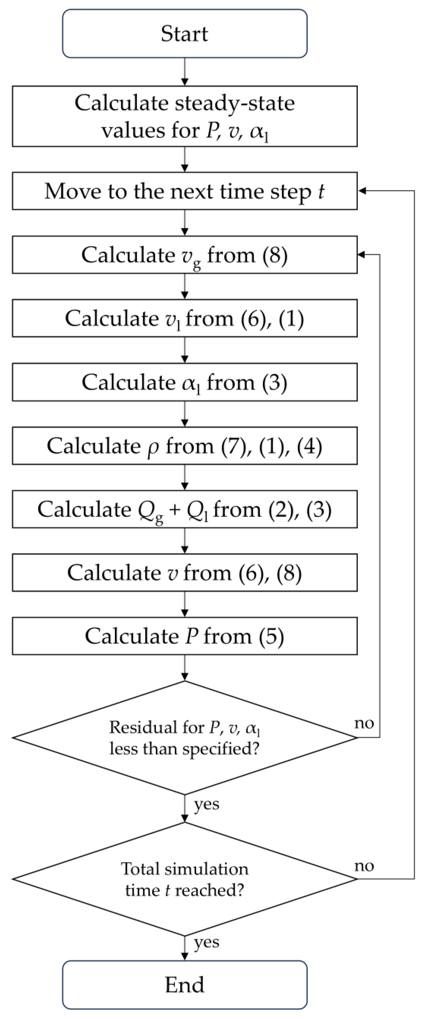
The drift–flux model of multiphase flow in a wellbore and pipelines is represented by a system of hyperbolic and algebraic equations, Equations (1)–(8), with the solution relying on the methods of computational fluid dynamics. Several numerical methods are widely used today to handle such problems, among which iterative approaches occupy a special place, including the following: SIMPLE (Semi-Implicit Method for Pressure-Linked Equations), SIMPLER (SIMPLE Revised), PISO (Pressure-Implicit with Splitting of Operators), etc. [35]. In this work, a numerical scheme is applied that is based on an iterative algorithm inspired by SIMPLE and adapted to the specifics of the selected drift–flux model. Despite the variety of numerical schemes available, all of them start with the spatial discretization of the simulation domain into a finite number of grid blocks or control volumes and subsequent integration of the governing equation over these grid blocks.
To solve the system of Equations (1)–(8), a numerical scheme that is implicit in time is used. In particular, a fixed time step Δt is selected, then the time derivatives in Equations (2), (3) and (5) are approximated with the differences between the values of the corresponding quantities at the current moment of time t and the previous moment t − Δt, divided by Δt. The remaining terms and derivatives included in (1)–(8) are evaluated at the current time step t. Then, (1)–(8) are reduced to a system of non-linear algebraic equations, where the non-linearity is handled through the iterative approach. As an initial guess for the variables P, v and αl, the corresponding values at the previous moment of time t − Δt are chosen. Then, the following algorithm (also shown in Figure 2) is iteratively repeated until the values of P, v and αl converge (that is, the relative changes at the end of each iteration compared to its beginning are less than a threshold, which in this work equals to 10−5):
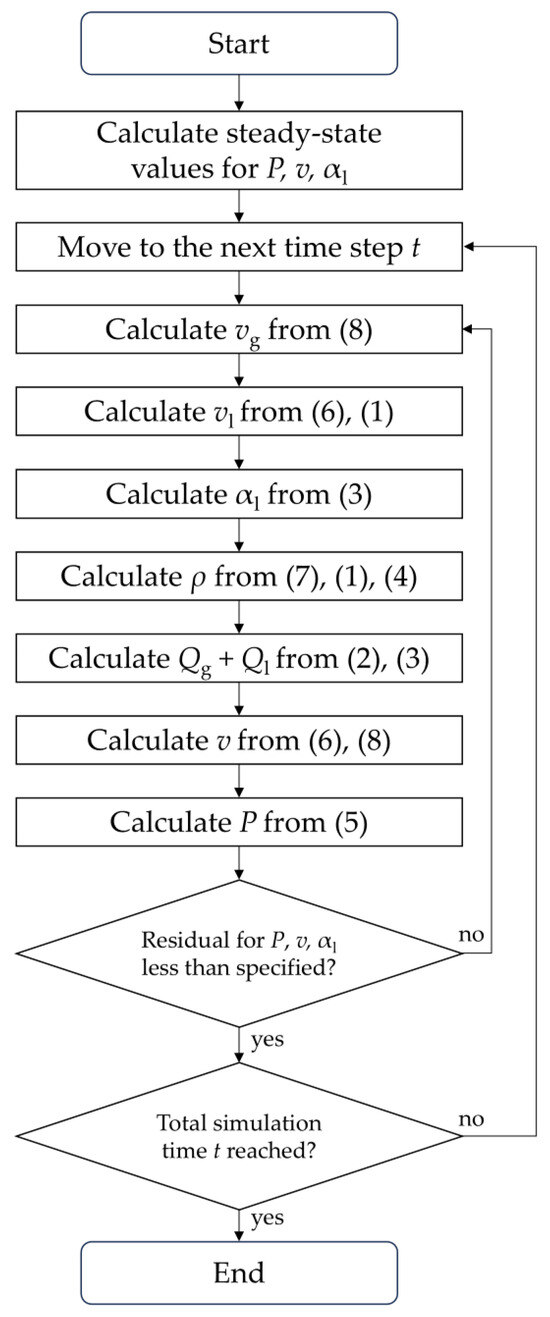
Figure 2.
Schematic description of the algorithm for solving the direct problem.
- (1)
- From Equation (8), vg is calculated;
- (2)
- From Equation (6), taking into account (1) and the found value of vg, vl is calculated;
- (3)
- From Equation (3), a new approximation for αl is found;
- (4)
- From Equation (7), taking into account (1) and (4), ρ is calculated;
- (5)
- The total mass flow rate is calculated by adding Equations (2) and (3), which leads to the values of Qg + Ql for all grid points of the well;
- (6)
- From the found values of the total mass rate, as well as algebraic Equations (6) and (8), the velocities v, vg and vl are found. These values are used as a new approximation for v;
- (7)
- A new approximation for P is found from Equation (5).
Note that during steps 3, 5 and 7 a system of linear differential equations is solved. Step 7 is introduced as the attempt to calculate P from relation (5) directly by integrating over the x coordinate for fixed values of ρ found convergence of the iterations. Instead, the value of the density ρ should be expressed in terms of the pressure P using Equations (4) and (7), as a result of which (5) transforms into a linear equation that includes both the derivative and the value P itself. Both the described solver and all the subsequent algorithms were implemented in the Python language using the “numpy” (version 1.22.4), and “scipy” (version 1.7.3.) libraries.
The well configuration consists of a deviated segment of length 1000 m discretized by a uniform grid with a size of 20 m for each grid block. The total time during which changes in the flow parameters were recorded was about 20 min, with the value of Δt selected in the range from 12.5 s to 50 s depending on how rapidly the values of Qg(x = L, t) and Ql(x = L, t) changed in the processes being investigated. The following values of physical and closure parameters were also adopted: ρl = 850 kg/m3, μ = 0.016 kg/mol, T = 300 K, g = 9.8 m/s2, θ = 70°, f = 0.005 m−1, d = 0.1 m, C = 1.2, and vd = 0.4 m/s. These values correspond to the conditions of a typical oil-producing well, which have been selected to demonstrate the feasibility of the proposed approach.
4. Case of Constant Pressure at the Wellhead
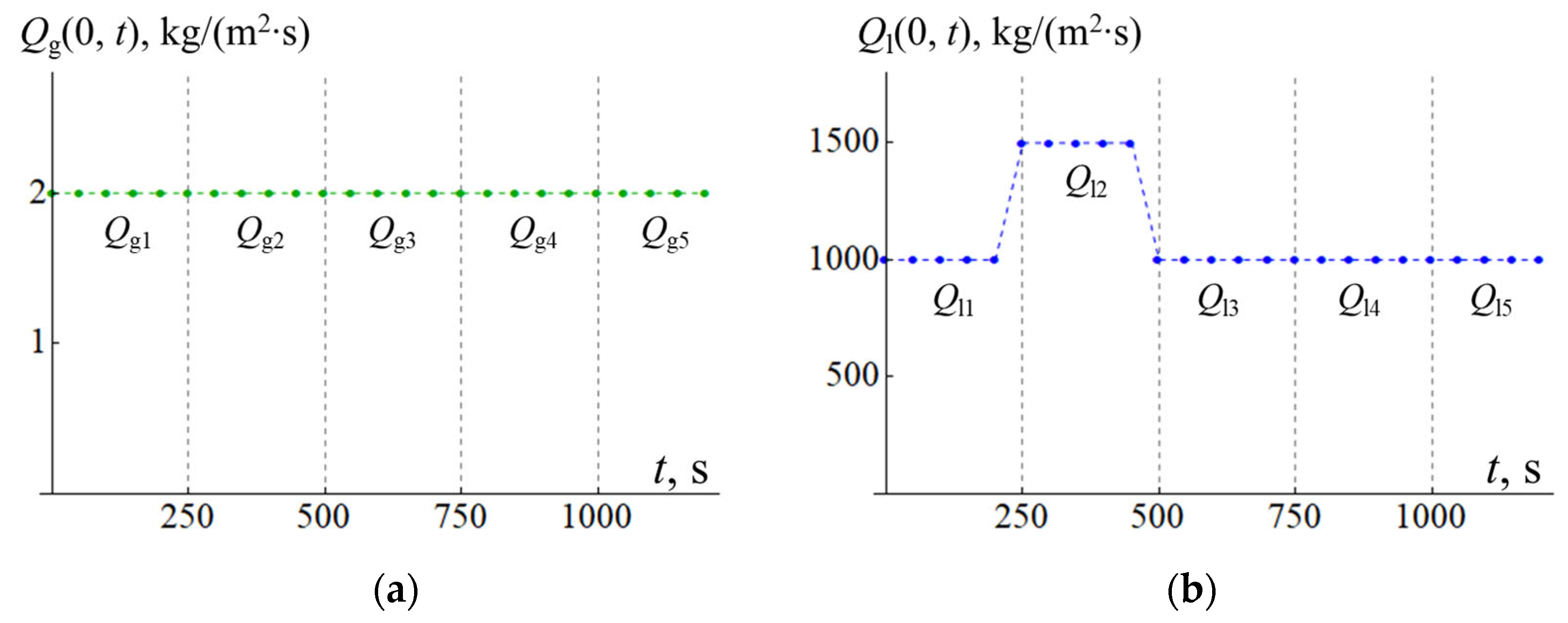
Firstly, the case considered is when the pressure at the wellhead is fixed, so that P(x = L, t) ≡ P0 (specifically, the value P0 = 1 atm is chosen). The inflows at downhole conditions Qg,l(x = 0, t) are represented by the known piecewise constant functions. It is assumed that the values of the inflows can change only at equal time intervals k × Δt, where k is some natural number; choosing for certainty k = 5 and Δt = 50 s, leads to k × Δt = 250 s. Then, the system is monitored for n = 5 such steps, that is, over a time interval of 0 ≤ t ≤ (k × n − 1)Δt = 1200 s, the dependence of each of the inflows on time will be completely determined by only n different values. The notations Qgi and Qli are introduced for these quantities, where the index i = 1, 2, …, n indicates the number of the “jump”, so that, for example, Qgi is a constant value of gas inflow at k × (i − 1)Δt ≤ t < k × i × Δt. Then, the array of 2n values, including both Qgi and Qli, will be targeted when estimating the inflow in the well.
4.1. Formulation of the Inverse Problem for Constant Wellhead Pressure
Firstly, the scenario with a minimum number of measurements is considered. This scenario assumes the availability of a flow meter at the wellhead, thus, the flow rates Qg,l(x = L, t) can be measured during the time of flow monitoring. The notation is introduced to indicate the reference to the measured values. If the multiphase model can accurately describe the flow process, then the correctly selected inflow values Qg,l(x = 0, t) used as the boundary condition for Equations (1)–(8) would lead to values of fluid flow rates at the wellhead that are close to the measured ones: . This can be formulated mathematically such that for certain Qg,l(x = 0, t) the residual of the following form should be minimal:
where the summation is carried out over each phase (f = g for gas and f = l for oil), as well as over all time instants t for which both measurement and numerical simulation results of flow variables based on the selected model do exist (for simplicity, it is assumed that this requirement is met by all moments of time for which the numerical calculation is carried out, i.e., the values t = 0, Δt, 2Δt, …). It is clear that the residual (9) is a function of the quantities Qgi and Qli, which completely define the time dependence of the piecewise constant inflows Qg,l(x = 0, t). The values of such a residual function R(Qgi, Qli) can be calculated for arbitrary values of its arguments by numerically solving the system of Equations (1)–(8) and substituting the results into the relation (10); therefore, the residual R can be minimized by numerical methods, thereby obtaining the optimal values of the arguments Qg1, Qg2, …, Qgn, Ql1, Ql2, …, Qln,. For numerical minimization of a function of several variables, the Nelder–Mead method [36] is used—a Simplex method that allows finding a local minimum of a function without calculating its derivatives, which would be especially difficult in the case of the implicitly defined function (9). Both the Nelder–Mead method and the drift–flux model are well-established methods; however, it is a combination of both that outlines the novelty of the presented work.
In the scenario where the maximum number of measurements is available, there are also several pressure gauges installed along the length of the well in addition to the flow meter. This enables the expansion of the residual R with the results of the measured pressure at different locations in the well. In this case, the residual function will have the following form:
Here, x1, x2, …, xm are the coordinates of the points where the pressure sensors are located (it is assumed that these points coincide with the grid nodes of the computational mesh along the x coordinate), m is the number of grid blocks and w is a constant weighting coefficient that defines the relative contribution of flow and pressure measurements to the resulting residual. Strictly speaking, the specific value of w should be chosen depending on the relationship between the errors of the corresponding measurements. However, the form of representation of the residual (10) is such (sum of squared relative deviations instead of absolute ones with a normalization factor 1/m), which allows approximately fixing the weighting coefficient, choosing, for example, w = 1. Numerical minimization of the residual (9) or (10) is the basis for assessing the fluid inflow at a constant pressure at the wellhead and a piecewise constant dependence of the inflow on time. Note that the problem of estimating inflows that depend continuously on time is a special case of the problem under consideration, provided that the time interval between successive changes in the values of Qg,l(x = 0, t) is Δt (that is, for m = 1). However, in such cases, the use of the Kalman filter and its variations may be more appropriate due to the comparatively higher resource intensity of the optimization approach proposed here (to be specific, solving one optimization problem took 5–6 h on a desktop PC with the selected grid parameters).
4.2. Simulation Results for Homogeneous Model
The application of the described method of inflow estimation is demonstrated with the test case based on the simulated data. This is described by a flow process in which the gas inflow remains constant throughout all the simulation time, that is, Qg(x = 0, t) ≡ 2 kg/(m2·s), and the oil inflow Ql(x = 0, t) is characterized by a single steplike disturbance, where the initial value increases from 1000 kg/(m2·s) to 1500 kg/(m2·s), and then returns to the previous value. The graphs of the functions Qg,l(x = 0, t) for this case are shown in Figure 3, where the dots indicate the values at moments of time t, spaced apart by Δt = 50 s. Solving the system of Equations (1)–(8), taking into account the corresponding boundary conditions, the data for and are obtained, which are the results of measuring the flow rates at the wellhead and the pressure at various points in the well. Further, these data are considered to be known and, based on them, the values of Qgi and Qli are calculated through the optimization process outlined in the previous section. It is easy to see from Figure 3 that their true values are equal to Qgi = 2 kg/(m2·s) for arbitrary values of index 1 ≤ i ≤ 5, as well as Qli = 1000 kg/(m2·s) for i ≠ 2 and Ql2 = 1500 kg/(m2·s). Obviously, it is how close the obtained estimated values Qgi and Qli are to the actual measured ones which can be considered as an indicator of the applicability of the developed approach.
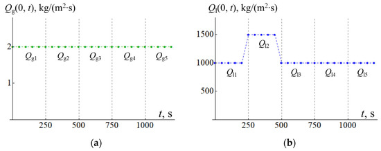
Figure 3.
Graphical representation of inflows of gas Qg(x = 0, t) (a) and oil Ql(x = 0, t) (b) as a function of time t. The vertical dashed lines show the moments of time t at which the inflow values can change abruptly.
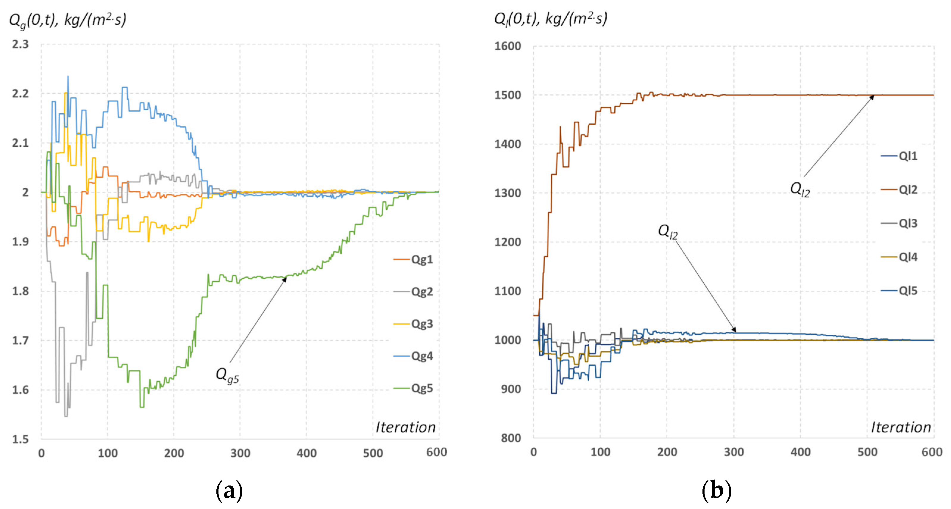
The process of numerical optimization of the residual (9) for the scenario with the minimum number of sensors is shown in Figure 4. The graphs show the change in the target values Qgi and Qli for 600 iterations through the optimization, after which no significant adjustments to the values of the optimized parameters are observed. As an initial approximation for Qgi and Qli, their values observed at the initial time t = 0 were chosen; in practice, these values can indeed be considered known, since before any disturbances in the inflow or pressure in the well, the constant values of Qg,l(x = 0, t) should obviously coincide with the flow rates Qg,l(x = L, t), which are measured at the wellhead. It follows from Figure 4 that the values of all the target variables are reconstructed with good accuracy, with the exception of the value of Qg5, which characterizes the gas inflow at the final stage of the flow process. Its calculated value Qg5 ≈ 2.012 kg/(m2·s) differs from the measured one by 0.61%, which seems insignificant but reflects an important feature of the inflow Qg,l(x = 0, t) estimation based solely on the flow rates Qg,l(x = L, t) without using additional information. It is clear that arbitrary inflow disturbances will affect the phase flow rates at the wellhead with some delay due to the finite propagation speed of the disturbances in the well. Consequently, the flow rate values Qg,l(x = L, t), known up to a certain time t = t1, carry information about the inflows Qg,l(x = 0, t) only up to the time t = t2 < t1. In this case, in the time interval t2 < t < t1, the values of the inflows can be almost arbitrary, unless some additional restrictions from physical considerations are imposed. In the case under consideration, the role of such a restriction is played by the piecewise constant nature of the change in Qg,l(x = 0, t), as a result of which the values of the inflows in the interval t2 < t < t1 turn out to be strongly connected with their values at earlier moments in time. Thus, the calculation of the values Qg5 and Ql5 becomes fundamentally possible. However, the number of terms in the residual (9) that depend on these quantities will be relatively small (their contribution will correspond to only a few terms related to the latest time t), which can lead to a decrease in the quality of the estimate of Qg5 and Ql5 in comparison with the remaining quantities Qgi and Qli that determine the inflow at earlier stages of the process. Table 1 summarizes the performance of the estimator in terms of the relative error reported for each time interval after 600 iterations. The relative error has been calculated according to Equation (11) below:
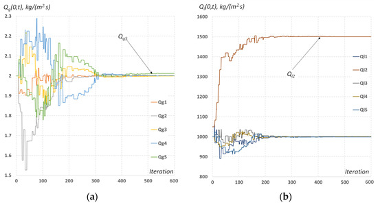
Figure 4.
(a) Estimated values of Qgi, defining the values of fluid inflow as a function of the iteration number in the process of numerical optimization with only the flowmeter available. (b) Estimated values of Qli, defining the values of fluid inflow as a function of the iteration number in the process of numerical optimization with only the flowmeter available.

Table 1.
Relative accuracy of estimated rates for the minimum information scenario.
It is calculated at each iteration for each phase (with f = g for gas and f = l for oil).
Figure 5 shows graphs similar to those shown in Figure 4, but for the scenario with the maximum number of sensors available. It is easy to see that in this case, certain difficulties associated with estimating the values of Qg5 and Ql5 at the final time interval also appear: the last 300 iterations of the optimizer, in essence, solve the problem of refining these two values, although the inflow at earlier time intervals has already been established with acceptable accuracy. However, the presence of the additional information that comes from pressure sensors located in the immediate vicinity of the point x = 0 allows the ultimate convergence of the required Qg5 and Ql5 to the correct values, with the relative errors of 0.12% and 0.17%, respectively. From this, a general conclusion can be drawn that, for rapid estimation of inflow, at least one downhole pressure sensor located near the inflow zone is required, since only in this case can data on inflow changes be recorded without delay. Table 2 summarizes the performance of the estimator in terms of the relative error reported for each time interval after 600 iterations.
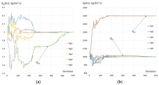
Figure 5.
(a) Estimated values of Qgi, defining the values of fluid inflow as a function of the iteration number in the process of numerical optimization with the flowmeter and pressure gauges available. (b) Estimated values of Qli, defining the values of fluid inflow as a function of the iteration number in the process of numerical optimization with the flowmeter and pressure gauges available.
Table 2.
Relative accuracy of estimated rates for the maximum information scenario.
5. Case of Variable Pressure at the Wellhead
In cases where the well operating mode is adjusted by maintaining a certain pressure at the wellhead, which is technically implemented, for example, by changing the power of the pump or manually adjusting the wellhead choke, the wellhead pressure P(x = L, t) can be considered a piecewise constant function of time rather than inflows Qg,l(x = 0, t). In this case, the inflows should be determined from a detailed solution to this problem based both on a model of fluid filtration in the near-wellbore region and upscaled models describing the geological properties of the entire reservoir. However, for application purposes, the simplified form is selected, in which the reservoir pressure Pr in the reservoir is considered known and the fluid inflows are linearly dependent on the pressure difference between the reservoir and the well [37], so that
where Jg and Jl are constant well productivity indices (normalized to the area of its cross-section), related to gas and oil, respectively. Adding relation (12) to the system of Equations (1)–(8) allows the mathematically correct formulation of the problem of calculating the parameters of the flow of a multiphase fluid in the case where only the dependence P(x = L, t) of the pressure at the wellhead on time is given. In this case, the quantities Qg,l(x = 0, t) should still be used as boundary conditions, but their values are determined indirectly from relation (12). It is clear that the abrupt change in pressure P(x = L, t) at the wellhead does not lead to a similar piecewise constant change in pressure P(x = 0, t) at the bottomhole. Consequently, the inflows Qg,l(x = 0, t) can also be characterized by rather complex transient behavior, which facilitates the need to adapt the proposed method of inflow estimation to the new conditions of the problem.
5.1. Features of Solving the Direct Problem
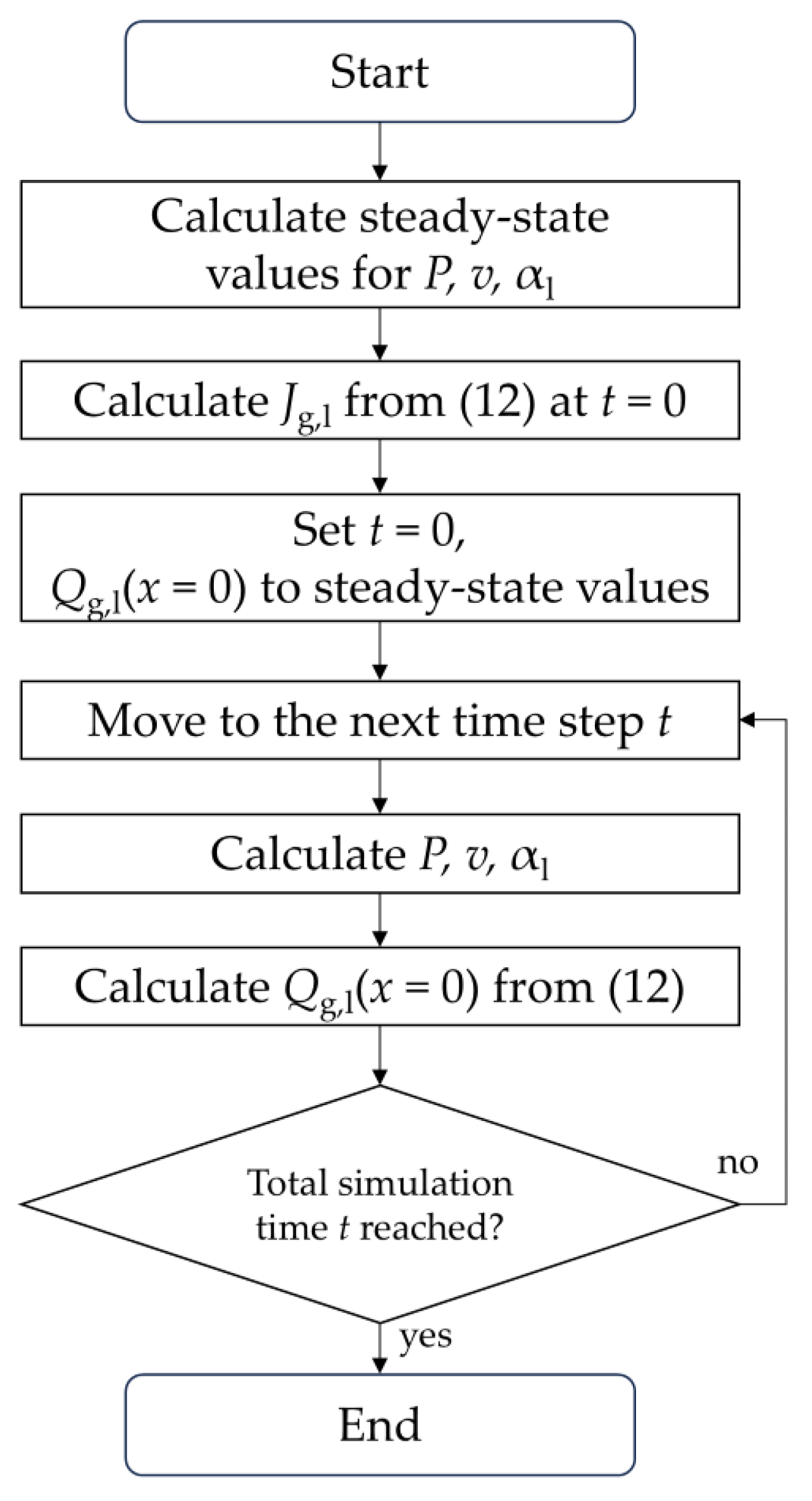
As it follows from the initial conditions, the distribution of multiphase rates along the well is uniform, that is, the values of Qg,l(x, t) are the same at all points in the well, so that measuring the flow rates Qg,l(x = L, t) at the wellhead allows the establishment of the values Qg,l(x = 0, t) of inflows. Thus, Equation (12) at t = 0 imposes restrictions on the possible values of the included parameters; in particular, the ratio of the productivity indices is fixed: Jg/Jl = Qg(L, 0)/Ql(L, 0). Instead of evaluating whether the rates Qg,l(x = L, t) recorded at the wellhead are consistent with the conditions defined above, Equation (12) is considered for determining the values of Jg and Jl. This leads to the appearance of an additional step in the algorithm for solving the system of Equations (1)–(8), which must be performed immediately after finding the steady solution (that is, the initial conditions for the system under consideration): the obtained pressure P(x = 0, t = 0) is substituted into (12) and, based on the given values Qg,l(0, 0) = Qg,l(L, 0), the values of Jg,l are calculated. Further, these values are considered known and unchanged. Note that this approach will lead to physically correct results only under the condition P(x = 0, t = 0) < Pr, which must be checked separately. Note that the process discussed in this paragraph resembles the production well test process, where the well is firstly shut in and then allowed to produce at a constant flow rate while bottomhole pressure is recorded. The iterative method for solving the system (1)–(8) allows relation (12) to be taken into account, along with the other equations of the system, successively refining the values of the parameters P, v and αl, which would simultaneously satisfy each of the equalities (1)–(8) and (12) for a given t. However, this approach seems redundant, since acceptable accuracy can be obtained in a simpler way. Namely, the values of the inflow Qg,l(x = 0, t) at a given time can be fixed without updating them in the process of searching for successive approximations. These values are recalculated only after the completion of the iterations, when P, v and αl have already been established. Then, the value P(x = 0, t), calculated for a given t, is substituted into the relation (12), and the updated values of the inflows are used to calculate the flow parameters at the next moment of time t + Δt. It is easy to see that this approach is equivalent to replacing Qg,l(x = 0, t) with Qg,l(x = 0, t + Δt) on the left-hand side of equality (12). Thus, the numerical scheme used becomes semi-explicit in time, which places higher demands on the choice of the step Δt to maintain the stability of the calculation. In fact, even with the value Δt = 50 s, which was previously used in studying the case of constant wellhead pressure, the instability of the scheme in similar calculation conditions did not manifest itself in any way. The choice of a reduced time step Δt = 12.5 s for the case of variable pressure was due to the fact that an abrupt change in wellhead pressure P(x = L, t) can lead to rather sharp changes in the flow rates Qg,l(x = L, t). For the remaining parameters of the system and the calculation scheme, the previous values were used; for the pressure in the reservoir, the value Pr = 30 atm was chosen. The numerical algorithm (also shown in Figure 6) outlined in this section is then summarized as follows:
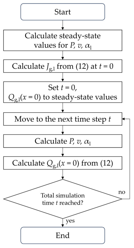
Figure 6.
Schematic description of the algorithm for solving the direct problem in the case of variable wellhead pressure.
- (1)
- From system (1)–(8), assuming that the flow is steady (all the time derivatives are equal to zero), the initial pressure distribution P(x = 0, t = 0) is calculated. The wellhead pressure P(x = L, t = 0) and flow rates are considered to be known.
- (2)
- Coefficients Jg and Jl are calculated from Equation (12) using the value of P(x = 0, t = 0) obtained at the previous step.
- (3)
- The initial values of inflow Qg,l(x = 0, t = 0) are assumed to be equal to the steady-state values of topside flow rates.
- (4)
- Using a boundary condition of wellhead pressure P(x = L, t) and inflow rates Qg,l(x = 0, t) at current time step t, the iterative process defined by steps 1–7 in Section 3.2 is performed, which leads to new values of P, v and αl.
- (5)
- With the calculated value of downhole pressure P(x = 0, t), updated values of the inflow rates Qg,l(x = 0, t + Δt) are obtained from Equation (12).
- (6)
- The steps 4–5 are repeated for all consequent time steps.
5.2. Formulation of the Inverse Problem for Variable Wellhead Pressure
Since it is the wellhead pressure P(x = L, t) which is the piecewise constant function of time in the case under consideration, the values P1, P2, …, Pn that should be chosen are the variables relative to which the residue R is minimized. In this case, the values Pi (i = 1, 2, …, n) are considered as the values of this pressure in the time interval k × (i − 1)Δt ≤ t < k × i × Δt, the duration of which at k = 15 is equal to k × Δt = 187.5 s. After the values of Pi are found as a result of minimizing the function R(P1, P2, …, Pn), solving the direct problem for the obtained dependence P(x = L, t) will allow the determination of the desired inflows Qg,l(x = 0, t). Note that residuals of the form (9) or (10) can be used regardless of what arguments they actually are functions of. This is due to the fact that all the main quantities included in these expressions for the residual R are either measurement results or the results of solving a direct problem, regardless of their specific formulation. Therefore, in the case of an abrupt change in pressure at the wellhead, it would also be possible to formally select the residual in both form (9) and form (10), which would correspond to the consideration of the two scenarios described above.
However, in the scenario with maximum data available, the presence of distributed pressure sensors in the well leads to the known values of P(x = L, t), which enables the direct calculation of the multiphase inflow rates. Of course, this may be only partially true, as the pressure sensors can be located far from the inflow location. However, this would highlight the necessity of installing additional gauges, which would facilitate direct measurement of the wellhead pressure with significantly greater reliability rather than estimating it with the multiphase fluid flow model. Therefore, only the scenario with minimum information available is considered in this chapter, when the residual R is presented in the form (9).
5.3. Simulation Results for Drift-Flux Model
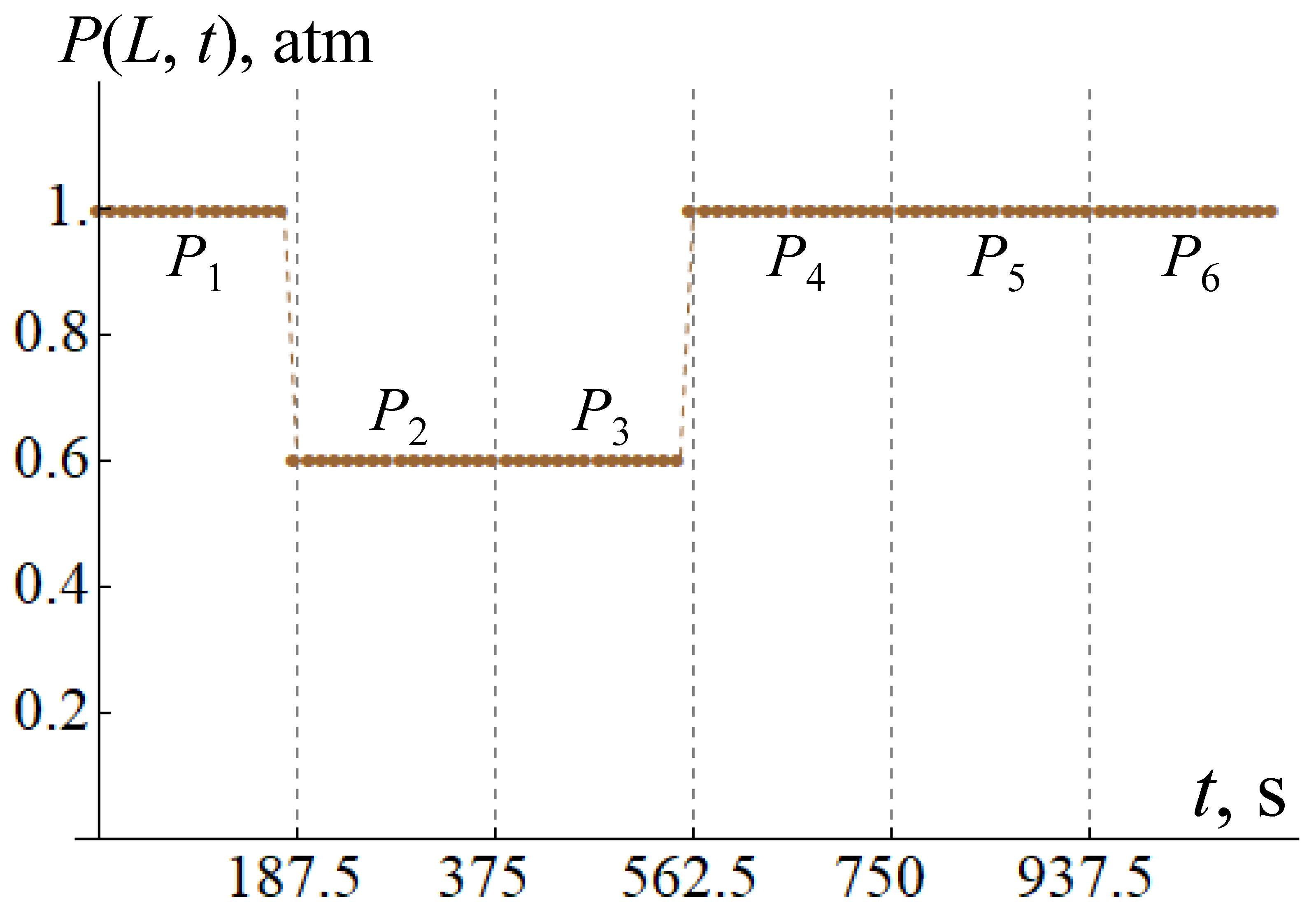
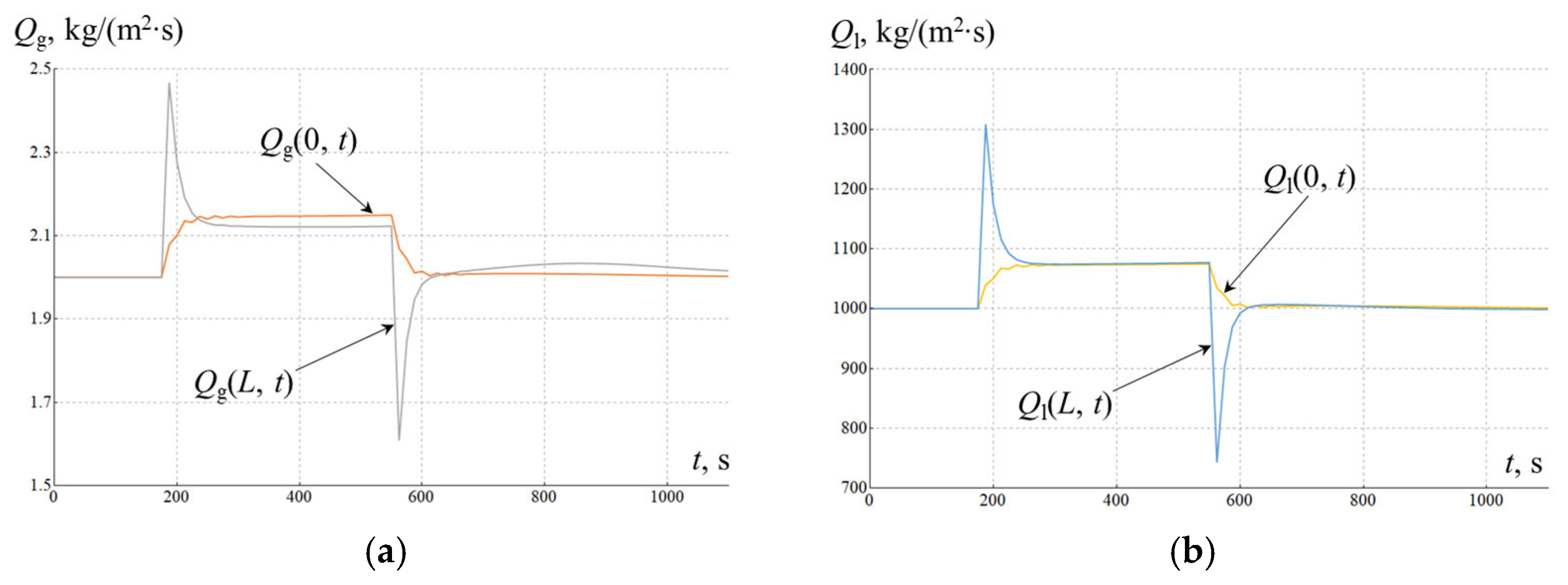
The simulated data is used again to mimic the results of measuring flow rates at the wellhead , which are obtained by solving the direct problem for the dependence P(x = L, t), shown in Figure 7 (similar to Figure 3, the points on the graph mark the values at moments of time t, separated from each other by Δt = 12.5 s). A dependence of this type can correspond, for example, to a process in which a submersible pump is switched on for a short time 2m × Δt = 375 s, after which it is switched off. This leads first to a decrease in pressure from P1 = 1 atm to P2 = P3 = 0.6 atm, and then to its increase to the previous value P4 = P5 = P6 = 1 atm. The calculated dependencies of the inflows Qg,l(x = 0, t) and flow rates at the wellhead Qg,l(x = L, t) for this case are shown in Figure 8. Next, the obtained flow rates Qg,l(x = L, t) are matched with the measurement results , and the inflows Qg,l(x = 0, t) are considered as desired target quantities.
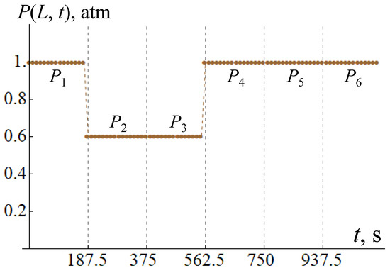
Figure 7.
Graphical representation of wellhead P(x = L, t) as a function of time. The vertical dashed lines indicated the moments of time t at which the inflow values change abruptly.

Figure 8.
Graphical representation of the inflows of gas Qg(x = 0, t) (a) and oil Ql(x = 0, t) (b) as a function of time t, as well as the flow rates at the wellheads Qg(x = L, t) and Ql(x = L, t) of gas and oil, respectively.
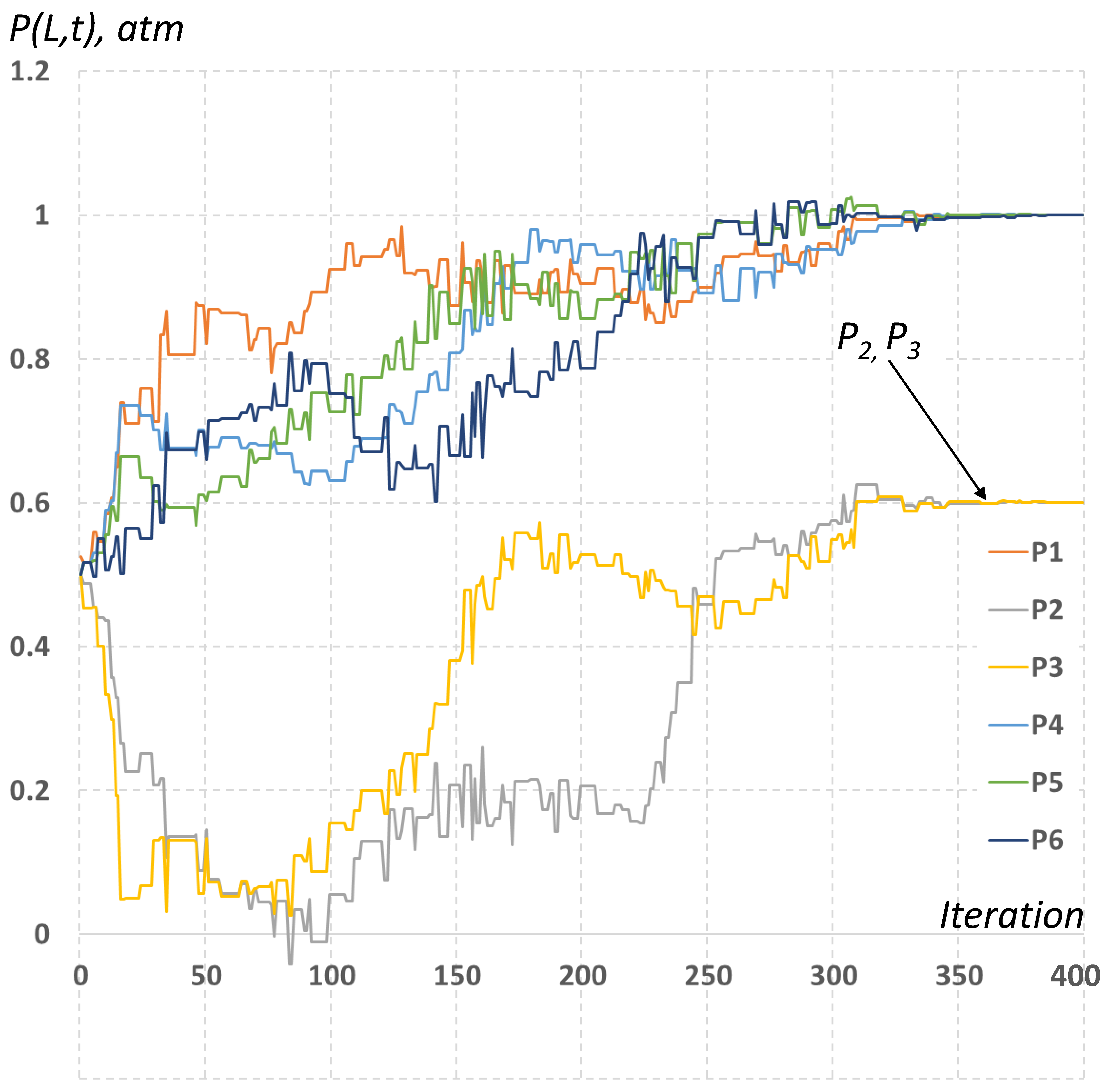
The process of numerical minimization of the residual (9) with respect to the parameters Pi, taking into account the selected values of , is illustrated in Figure 9. As an initial approximation for all parameters Pi, the same value Pi = 0.5 atm was used. It is easy to see that after 400 iterations, the Pi values practically stop changing and match with the target values with sufficient accuracy. Moreover, after 427 iterations, the mismatch between the calculated Pi values and the target ones appear only in the fifth decimal place. It is obvious that the subsequent solution of the direct problem based on the obtained Pi allows the establishment of the values of the inflows Qg,l(x = 0, t), which closely resemble the true values of the inflows, as shown in Figure 8. It should be noted that in this case, the previously discussed negative effects caused by the finite velocity of the disturbance propagation in the well did not manifest themselves in any way, although the inflows were estimated solely on the basis of measured fluid flow rates at the wellhead. Thus, knowledge of the piecewise constant nature of the pressure P(x = L, t) variation is an extremely important piece of a priori information.
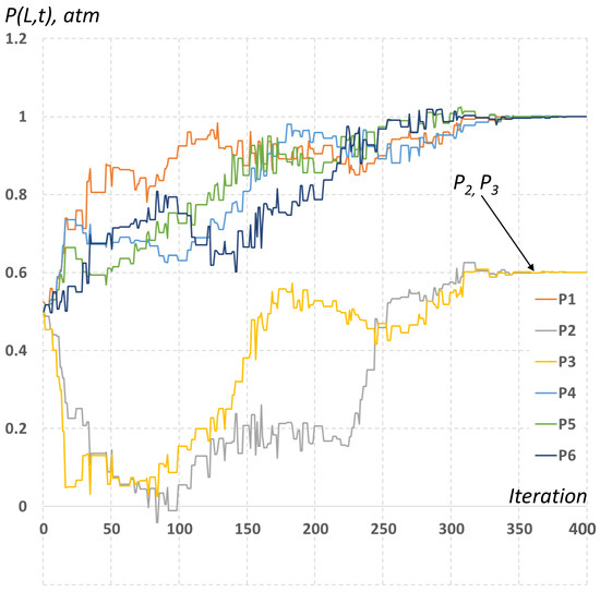
Figure 9.
Estimated values of wellhead pressure Pi values as a function of the iteration number in the process of numerical optimization.
6. Conclusions and Future Work
This paper presents a hybrid approach to estimate the inflow from the reservoir to the wellbore, which is based on the numerical minimization of a mismatch between model prediction and the data. As can be seen from the examples considered, the proposed method does indeed solve the estimation problem, with a demonstrated relative accuracy below 1% for all considered scenarios. This is a preliminary indication, and a detailed sensitivity analysis needs to be performed to obtain conclusive estimates on the accuracy of the developed approach.
From a practical point of view, the specifics of its implementation are such that the corresponding calculations are quite resource-intensive, which refers both to the solution of the system of equations describing the flow of a multiphase fluid and the numerical optimization. Nevertheless, this approach has a number of important advantages that can justify even a significant reduction in the computational efficiency. In particular, the technique based on the minimization of the residual allows naturally taking into account the constraints that can be imposed on the target variables or any intermediate parameters. In this paper, this type of restriction was introduced by the stepwise nature of the dependence of inflows or wellhead pressure on time.
Although the demonstrated results are promising, this work is a feasibility study, since a few more challenges need to be overcome before this method can be implemented in practice for oil and gas applications. As the multiphase wellbore flow is generally three-phase, accounting for water transport would enable handling of a wider range of wellbore operating conditions. Since three-phase inflow investigation will require more data, the investigation into the need for additional measurements has to be performed. Thermal measurements obtained through downhole gauges or distributed fiber optic temperature sensors are one of the options for such investigation. This would require the update of the flow model with the continuity equation for water phase and energy conservation law to account for temperature variation. Finally, a comparison between the optimization method and Kalman filtering is another important topic for future work.
Author Contributions
Conceptualization, A.G.; methodology, A.G. and E.M.; software, E.M.; validation, A.G. and E.M.; formal analysis, A.G. and E.M.; investigation, A.G. and E.M.; resources, A.G. and M.A.; data curation, M.A.; writing—original draft preparation, A.G. and E.M.; writing—review and editing, A.G., E.M., A.K. and M.A.; visualization, A.G. and E.M.; supervision, A.G. and A.K.; project administration, M.A. All authors have read and agreed to the published version of the manuscript.
Funding
This research received no external funding.
Data Availability Statement
The original contributions presented in the study are included in the article, further inquiries can be directed to the corresponding author.
Conflicts of Interest
Anton Gryzlov holds the position of Petroleum Engineering Consultant at Aramco Innovations, Eugene Magadeev holds the position of Research Scientist at Aramco Innovations and Andrey Kovalskii holds the position of Petroleum Scientist at Aramco Innovations. Muhammad Arsalan holds the position of Petroleum Engineering Consultant at Saudi Aramco. The authors declare that the research was conducted in the absence of any commercial or financial relationships that could be construed as a potential conflict of interest.
References
- Jansen, J.-D.; Douma, S.D.; Brouwer, D.R.; Van den Hof, P.M.J.; Bosgra, O.H.; Heemink, A. Closed Loop Reservoir Management. In Proceedings of the SPE Reservoir Simulation Symposium Proceedings, The Woodlands, TX, USA, 2–4 February 2009; pp. 856–873. [Google Scholar] [CrossRef]
- Jansen, J.-D.; Bosgra, O.H.; Van den Hof, P.M.J. Model-based control of multiphase flow in subsurface oil reservoirs. J. Process Control 2008, 18, 846–855. [Google Scholar] [CrossRef]
- Hansen, L.S.; Pedersen, S.; Durdevic, P. Multi-Phase Flow Metering in Offshore Oil and Gas Transportation Pipelines: Trends and Perspectives. Sensors 2019, 19, 2184. [Google Scholar] [CrossRef]
- Meribout, M.; Azzi, A.; Ghendour, N.; Kharoua, N.; Khezzar, L.; AlHosani, E. Multiphase flow meters targeting oil & gas industries. Measurement 2020, 165, 108111. [Google Scholar] [CrossRef]
- Falcone, G.; Hewitt, G.F.; Alimonti, C.; Harrison, B. Multiphase flow metering: Current trends and future developments. J. Pet. Technol. 2002, 54, 77–84. [Google Scholar] [CrossRef]
- Manzar, M.A.; Sun, D.; Chace, D. Refining interpretation models of multiphase flow for existing and next-generation production logging sensors. Petrophysics 2018, 59, 439–456. [Google Scholar] [CrossRef]
- Duthie, L.S.; Saiood, H.A.; Al-Anizi, A.A.; AlGhamdi, T.A. A comparative review of production logging techniques in open hole extended reach wells. In Proceedings of the SPE Asia Pacific Oil & Gas Conference and Exhibition, Virtual, 17–19 November 2020. [Google Scholar] [CrossRef]
- Fortuna, L.; Graziani, S.; Rizzo, A.; Xibilia, M.G. Soft Sensors for Monitoring and Control of Industrial Processes; Springer: London, UK, 2007. [Google Scholar]
- Bikmukhametov, T.; Jäschke, J. First principles and machine learning virtual flow metering: A literature review. J. Pet. Sci. Eng. 2019, 184, 106487. [Google Scholar] [CrossRef]
- Andrianov, N.A. Machine Learning Approach for Virtual Flow Metering and Forecasting. In Proceedings of the 3rd IFAC Workshop on Automatic Control in Offshore Oil and Gas Production, Esbjerg, Denmark, 30 May–1 June 2018. [Google Scholar]
- Spesivtsev, P.; Sinkov, K.; Sofronov, I.; Zimina, A.; Umnov, A.; Yarullin, R.; Vetrov, D. Predictive model for bottomhole pressure based on machine learning. J. Pet. Sci. Eng. 2018, 166, 825–841. [Google Scholar] [CrossRef]
- Bikmukhametov, T.; Jäschke, J. Oil Production Monitoring using Gradient Boosting Machine Learning Algorithm. IFAC-PapersOnLine 2019, 52, 514–519. [Google Scholar] [CrossRef]
- Gryzlov, A.; Mironova, L.; Safonov, S.; Arsalan, M. Artificial Intelligence and Data Analytics for Virtual Flow Metering. In Proceedings of the SPE Middle East Oil & Gas Show and Conference, Sanabis, Bahrain, 28 November–1 December 2021. [Google Scholar] [CrossRef]
- Hotvedt, M.; Grimstad, B.; Ljungquist, D.; Imsland, L. On gray-box modeling for virtual flow metering. Control Eng. Pract. 2022, 118, 104974. [Google Scholar] [CrossRef]
- Andrade, G.M.P.; de Menezes, D.Q.F.; Soares, R.M.; Lemos, T.S.M.; Teixeira, A.F.; Ribeiro, L.D.; Vieira, B.F.; Pinto, J.C. Virtual flow metering of production flow rates of individual wells in oil and gas platforms through data reconciliation. J. Pet. Sci. Eng. 2022, 208, 109772. [Google Scholar] [CrossRef]
- Vanvik, T.; Henriksson, J.; Yang, Z.; Weisz, G. Virtual flow metering for continuous real-time production monitoring of unconventional wells. In Proceedings of the Unconventional Resources Technology Conference, Houston, TX, USA, 20–22 June 2022. [Google Scholar] [CrossRef]
- Bikmukhametov, T.; Jäschke, J. Combining machine learning and process engineering physics towards enhanced accuracy and explainability of data-driven models. Comput. Chem. Eng. 2020, 138, 106834. [Google Scholar] [CrossRef]
- Lorentzen, R.J.; Nævdal, G.; Lage, A.C.V.M. Tuning of parameters in a two-phase flow model using an ensemble Kalman filter. Int. J. Multiph. Flow 2003, 29, 1283–1309. [Google Scholar] [CrossRef]
- Shoham, O. Mechanistic Modeling of Gas-Liquid Two-Phase Flow in Pipes; Society of Petroleum Engineers: Richardson, TX, USA, 2013. [Google Scholar]
- Masella, J.M.; Tran, Q.H.; Ferre, D.; Pauchon, C. Transient simulation of two-phase flows in pipes. Int. J. Multiph. Flow 1998, 24, 739. [Google Scholar] [CrossRef]
- Kalman, R.E. A new approach to linear filter and prediction problems. J. Basic Eng. 1960, 82, 35–45. [Google Scholar] [CrossRef]
- Leskens, M.; de Kruif, B.; Belfroid, S.; Smeulers, J.; Gryzlov, A. Downhole multiphase metering in wells by means of soft-sensing. In Proceedings of the Intelligent Energy Conference and Exhibition, Amsterdam, The Netherlands, 25–27 February 2008. [Google Scholar]
- Aamo, O.M.; Eikrem, G.O.; Siahaan, H.B.; Foss, B.A. Observer design for multiphase flow in vertical pipes with gas lift—theory and experiments. J. Process Control 2004, 15, 247. [Google Scholar] [CrossRef]
- Bloemen, H.H.J.; Belfroid, S.P.C.; Sturm, W.L.; Verhelst, F.J.P.C.M.G. Soft sensing for gas-lift wells. SPE J. 2006, 11, 454. [Google Scholar] [CrossRef]
- Muradov, K.M.; Davies, D.R. Zonal rate allocation in intelligent wells. In Proceedings of the SPE Intelligent Energy Conference, Utrecht, The Netherlands, 8–11 June 2009. [Google Scholar]
- Nævdal, G.; Vefring, E.; Berg, A.; Mannseth, T.; Nordtvedt, J.E. A new methodology for the optimization of the placement of downhole production-monitoring sensors. SPE J. 2001, 6, 108. [Google Scholar] [CrossRef]
- Lorentzen, R.J.; Sævareid, O.; Nævdal, G. Soft multiphase flow metering for accurate production allocation. In Proceedings of the SPE Russian Oil and Gas Conference and Exhibition, Moscow, Russia, 26–28 October 2010. [Google Scholar]
- Wang, G.; Lee, J.; Thigpen, B.; Vachon, G.; Poland, S.; Norton, D. Modeling Flow Profile Using Distributed Temperature Sensor (DTS) System. In Proceedings of the Intelligent Energy Conference and Exhibition: Intelligent Energy, Amsterdam, The Netherlands, 25–27 February 2008. [Google Scholar] [CrossRef]
- Muradov, K.; Davies, D. Application of Distributed Temperature Measurements to Estimate Zonal Flow Rate and Pressure. In Proceedings of the International Petroleum Technology Conference, Bangkok, Thailand, 15–17 November 2012. IPTC 2012. [Google Scholar] [CrossRef]
- Stewart, H.B.; Wendroff, B. Review article; two-phase flow: Models and methods. J. Comput. Phys. 1984, 56, 363–409. [Google Scholar] [CrossRef]
- Spesivtsev, P.; Sinkov, K.; Osiptsov, A. Comparison of Drift-flux And Multi-fluid Approaches to Modeling of Multiphase Flow In Oil And Gas Wells. WIT Trans. Eng. Sci. 2013, 79, 89–99. [Google Scholar] [CrossRef]
- Osiptsov, A.; Sinkov, K.; Spesivtsev, P. Justification of the drift-flux model for two-phase flow in a circular pipe. Fluid Dyn. 2014, 49, 614–626. [Google Scholar] [CrossRef]
- Haaland, S.E. Simple and explicit formulas for the friction factor in turbulent pipe flow. J. Fluids Eng. 1983, 105, 89. [Google Scholar] [CrossRef]
- Shi, H.; Holmes, J.A.; Diaz, L.R.; Durlofsky, L.J.; Aziz, K. Drift-flux parameters for three-phase steady-state flow in wellbores. SPE J. 2005, 10, 130–137. [Google Scholar] [CrossRef]
- Versteeg, H.K.; Malalasekera, W. An introduction to computational fluid dynamics. In The Finite Volume Method; Pearson Education Ltd.: Harlow, UK, 2007. [Google Scholar]
- Nelder, J.A.; Mead, R. A Simplex Method for Function Minimization. Comput. J. 1965, 7, 308. [Google Scholar] [CrossRef]
- Alarifi, S.; Alnuaim, S.; Abdulraheem, A. Productivity index prediction for oil horizontal wells using different artificial intelligence techniques. In Proceedings of the SPE Middle East Oil & Gas Show and Conference, Manama, Bahrain, 8–11 March 2015. [Google Scholar]

Disclaimer/Publisher’s Note: The statements, opinions and data contained in all publications are solely those of the individual author(s) and contributor(s) and not of MDPI and/or the editor(s). MDPI and/or the editor(s) disclaim responsibility for any injury to people or property resulting from any ideas, methods, instructions or products referred to in the content. |
© 2025 by the authors. Licensee MDPI, Basel, Switzerland. This article is an open access article distributed under the terms and conditions of the Creative Commons Attribution (CC BY) license (https://creativecommons.org/licenses/by/4.0/).