Hybrid Symbolic Regression and Machine Learning Approaches for Modeling Gas Lift Well Performance

Abstract

Proper determination of the bottomhole pressure in a gas lift well is essential to enhance production, tackle operating concerns, and use the least amount of gas. Mechanistic models, empirical correlation, and hybrid models are usually limited by the requirements for calibration, large amounts of inputs, or limited scope of work. Through this study, sixteen well-tested machine learning (ML) models, such as genetic programming-based symbolic regression and neural networks, are developed and studied to accurately predict flowing BHP at the perforation depth, using a dataset from 304 gas lift wells. The dataset covers a variety of parameters related to reservoirs, completions, and operations. After careful preprocessing and analysis of features, the models were prepared and tested with cross-validation, random sampling, and blind testing. Among all approaches, using the L-BFGS optimizer on the neural network gave the best predictions, with an R² of 0.97, low errors, and better accuracy than other ML methods. Upon using SHAP analysis, it was found that the injection point depth, tubing depth, and fluid flow rate are the main determining factors. Further using the model on 30 unseen additional wells confirmed its reliability and real-world utility. This study reveals that ML prediction for BHP is an effective alternative for traditional models and pressure gauges, as it is simpler, quicker, more accurate, and more economical.

1. Introduction

1.1. The Importance of Predicting Bottomhole Pressure

A gas lift well is an artificial method used in the oil and gas field to produce more fluids, mainly when the reservoir pressure is low and fluids do not rise to the surface properly [1,2,3]. To use a gas lift system, high-pressure gas is injected into the wellbore through a special valve, which reduces the BHP [4,5,6]. With a lowered BHP, the movement of reservoir fluids into the wellbore is enabled [7,8,9]. The flowing BHP at the perforation depth in gas lift wells is essential to know for a number of reasons [10,11]. First, accurate BHP prediction enables better management of reservoir behavior, reservoir pressure, and well performance [12,13,14,15]. It supports optimal gas injection rates, which are essential for maximizing production efficiency while minimizing gas usage [16,17]. Second, it also helps in determining if there is a problem with excessive liquid loading, malfunctioning gas lift valves, or formation damage [18,19]. Moreover, if many connected gas lift wells are relying on the same surface gas supply, accurate BHP predictions help to prevent any inefficiencies in gas management [20,21]. In addition, the well’s BHP at perforation depth lets engineers determine if the well needs a stimulation treatment or artificial lift system adjustment [22,23]. Having accurate BHP numbers is vital for producing more, operating safely, lowering expenses, and increasing the lifetime of the reservoir [24,25]. This means it plays a crucial role in designing and running gas lift systems [26,27,28].

1.2. Traditional Prediction Methods

To calculate the flowing BHP of a gas lift well, one must understand the hydrostatic head, fluid friction, and fluid acceleration [29,30]. The hydrostatic head is the result of pressure from the fluid column’s density [31,32]. Fluid friction reflects the loss of pressure as fluids move through the wellbore due to factors such as the tube roughness, internal diameter of the tube, fluid velocity, fluid density, length of the tube, and flow regime [33,34]. While it is usually less significant than the others, fluid acceleration must be considered when there is a sudden increase in flow speed, especially in high gas injection and high gas–oil ratio scenarios [35]. These components interact with well-specific variables like the gas–liquid ratio, water cut, wellhead pressure, operating gas injection pressure, injection point depth, and temperature gradients, making flowing BHP estimation a complex task that must capture the dynamic, multiphase flow conditions present in gas lift operations [36,37,38].

Traditional prediction methods for BHP in gas lift wells include physics-based models, empirical correlations, and hybrid models [39]. Physics-based models, particularly mechanistic multiphase flow models, such as those developed by Taitel and Dukler (1976) and Taitel et al. (1980), offer detailed and rigorous representations of fluid dynamics within wellbores [40,41,42]. They tend to perform well in making accurate predictions if the data they use are extensive and reliable. Yet, they are rarely used in big operations or real-time scenarios because running them requires powerful computers and a lot of time spent adapting them to the environment [43,44]. Field data-based correlations from Duns & Ros, Aziz et al., Mandhane et al., and Beggs & Brill (all published in 1963, 1972, 1974, and 1973) are easy to apply and fast, yet they may not give accurate results when applied in other regions [45,46,47]. Integrating physics models with empirically developed equations produces hybrid models that are flexible, accurate, and easier to use in many circumstances, but setting up and ensuring their accuracy can be complicated [48,49].

1.3. Machine Learning Models for Predicting BHP

Regression ML models serve to predict continuous results by spotting patterns in a set of data [50,51,52,53]. They are key tools in engineering because they can handle challenging, complicated, and high-dimensional data without demanding detailed and complicated physical formulations [54,55,56,57]. Although progress has been made in the oil and gas industry related to data-driven models in hydraulic fracturing [58,59,60,61,62], reservoir engineering [63,64,65], production engineering [66,67,68], and completion engineering [69,70,71] for the last several years, there is little work published on predicting BHP related to gas lift wells. Symbolic regression is an emerging way to construct equations from data that are understandable, and it often shows a competitive accuracy compared to black-box models [72,73]. It has been shown by recent studies that physics-informed machine learning methods combine the strengths of machine algorithms and physical science, thus making models both more reliable and accurate [74,75,76]. For example, Abdulwarith and Ammar et al. (2024) developed a hybrid model capable of predicting friction pressure losses during hydraulic fracturing with an error margin below 5%, thereby contributing to enhanced operational efficiency in fracturing processes [77].

More studies are needed to better understand what ML can do in predicting BHP in gas lift systems. Because of this missing advanced models, this study is designed to develop and compare sixteen advanced ML models using readily available field data. Although individual ML models to predict BHP have been examined in previous research, our research is unique in that it thoroughly benchmarks a variety of sixteen models, as well as provides interpretable symbolic regression and SHAP-based feature analysis. Such a scope of comparison, together with the blind testing and field data, improves the performance and explainability of ML methods on gas lift well modeling, providing a more scalable and interpretable option to conventional methods. There is less cost and time needed with machine learning models than with the common bottomhole pressure gauges, which often prove hard to place [78]. In addition, they outperform standard physics models, empirical solutions, and existing hybrid approaches in terms of accuracy, adjustment to many field conditions, and scalability [79,80,81]. Because they can process extensive data, they can more accurately estimate bottomhole pressure in real time and thereby improve both operational efficiency and decision making.

2. Methodology

Five steps are used as the methodology for this study, as shown in Figure 1. Each part of the process is improved according to established objectives and later applied to develop a model for predicting BHP in gas lift wells.

2.1. Data Collection

In this study, we used real data from 304 gas lift wells. The dataset includes the tubing inside diameter (TID), tubing depth (TD), perforation depth (PD), wellhead pressure (WHP), reservoir temperature (RT), gas–oil ratio (GOR), water cut (WC), and fluid flow rate (FFR). Other operational considerations, such as the operating gas injection pressure (OGIP), gas lift injection rate (GLIR), and injection point depth (IPD), are also used. The flowing bottomhole pressure (BHP) is what the model is trying to predict. The machine learning models were built from the compiled dataset and assessed by comparing their results to BHP measurements from the downhole pressure gauges used during the production test. These gauges were deployed via wireline during routine gas lift flow surveys to assess well performance under operational conditions. Initially, the study collects data from 304 gas lift wells in Egypt’s Western Desert, summing up to 3648 points.

Table 1. Summary statistics for the collected data.

Parameter	Units	MIN	MAX	AVG	Median
Tubing inside diameter	inches	2.441	2.992	2.731	2.992
Tubing depth	ft	3002	10,494	7022.441	7506
Perforation depth	ft	3052	10,544	7116.322	7656
Wellhead pressure	psi	30	250	109.4079	100
Reservoir temperature	f	110.52	185.44	151.1632	156.56
Gas–oil ratio	scf/stb	100	1600	654.9605	600
Water cut	%	0	99	71.21053	81.5
Operating gas injection pressure	psi	800	1100	912.5	900
Gas lift injection rate	mmscf/d	0.3	1.2	0.566447	0.5
Bottomhole pressure	psi	415	1669	830.2862	803.5
Injection point depth	ft	2304	9390	6099.862	6379.5
Fluid flow rate	stb/d	22	1963	730.2566	676

shows the parameters included in the datasets. For this study, all of the wells are vertical and produce from multiple formations under varying operating conditions. The gathered dataset is characterized by having an extensive range of completion specifications, properties of the reservoir, and operational parameters. This diversity is key to creating reliable regression-based machine learning models that can handle complex associations, achieve accurate predictions, reduce certain biases, and do well in various tasks.

The pair plot in Figure 2 shows the connections among the essential variables in the dataset meant for flowing BHP predictions. The distribution of each variable is plotted diagonally, and correlations between bivariate variables are plotted off the diagonal. There is a degree of linear correlation noted between bottomhole pressure (BHP) and TD, PD, RT, GOR, WC, and FFR, suggesting expected dependencies. It is notable that TD, RT, IPD, and PD are strongly linearly correlated, as this is common during normal gas lift operation. Looking at pair plots is necessary to notice patterns of correlation and similarities in the data, which are important for enhancing model performance and ensuring the inclusion of relevant, non-redundant input variables in ML models.

Figure 3 provides insights into how all the used parameters are distributed for estimating bottomhole pressure (BHP), using violin plots. Data along the x-axis contain the variables, and the y-axis displays normalized values that are limited to the range of 0 to 1. Both the box plot and kernel density estimate are shown with each violin plot, helping to present a brief statistical summary and the distribution of the data. The white line in the center represents the median, and the black bar above it outlines the middle 50% of the data (represented by the IQR). The sections of a violin are wide when there are numerous values grouped closely and narrower when there are fewer values grouped. Each outlier is drawn as a single point, unlike the rest of the density estimation. For all parameters, distributions are found to be substantially different. For example, TID highlights that there are two different groups of values, suggesting bimodality. There is a high level of symmetry, a dense appearance, and little variation in TD, PD, and RT. Both WHP and GLIR have wider ranges because they include more variation. The GOR and WC are tightly clustered, while OGIP has a narrow peak with barely any changes. BHP is fairly well spread, and IPD shows a slightly skewed distribution. There is a broad distribution in the FFR column, indicating significant variability in fluid production rates across the wells in the dataset.

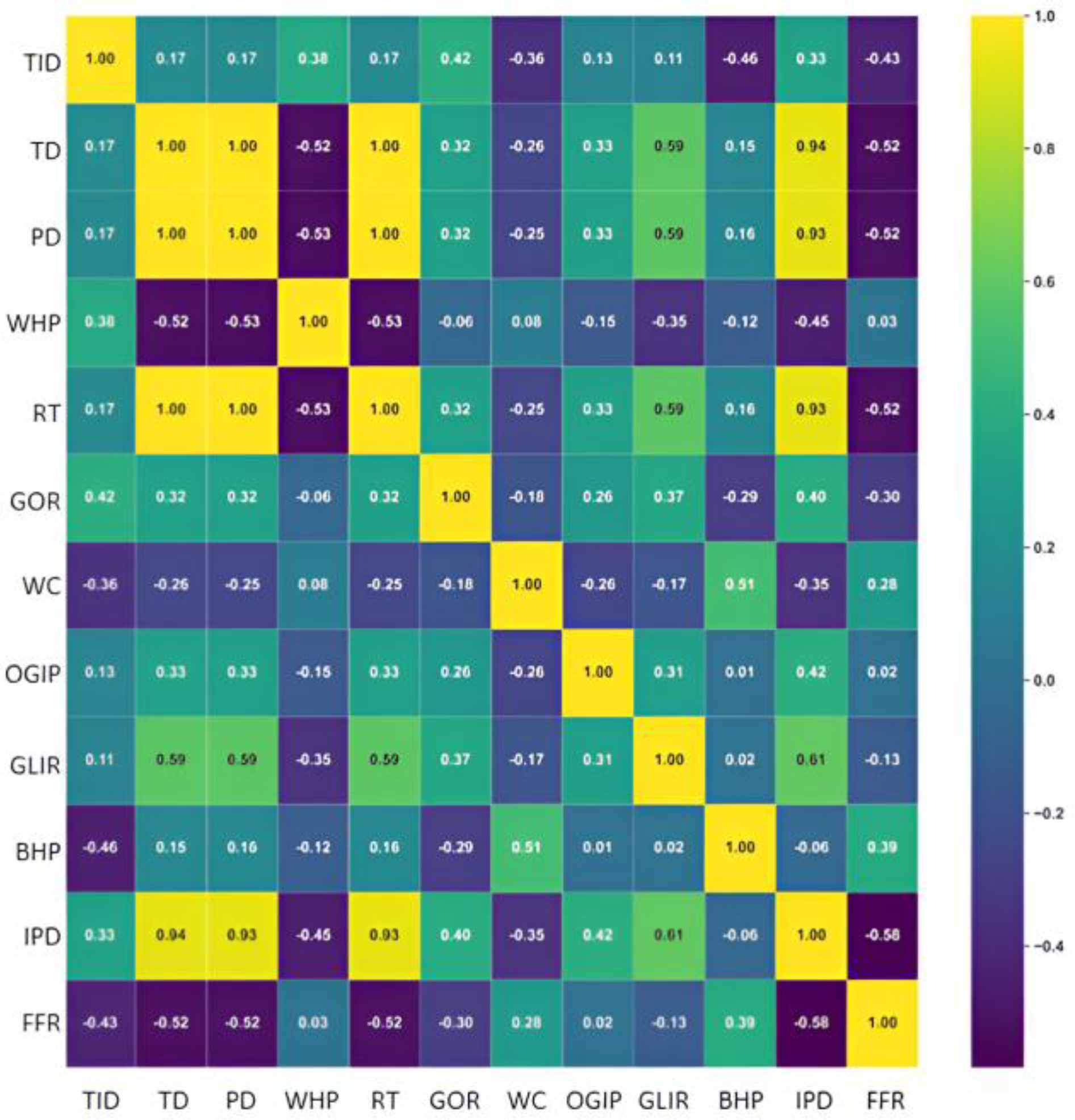
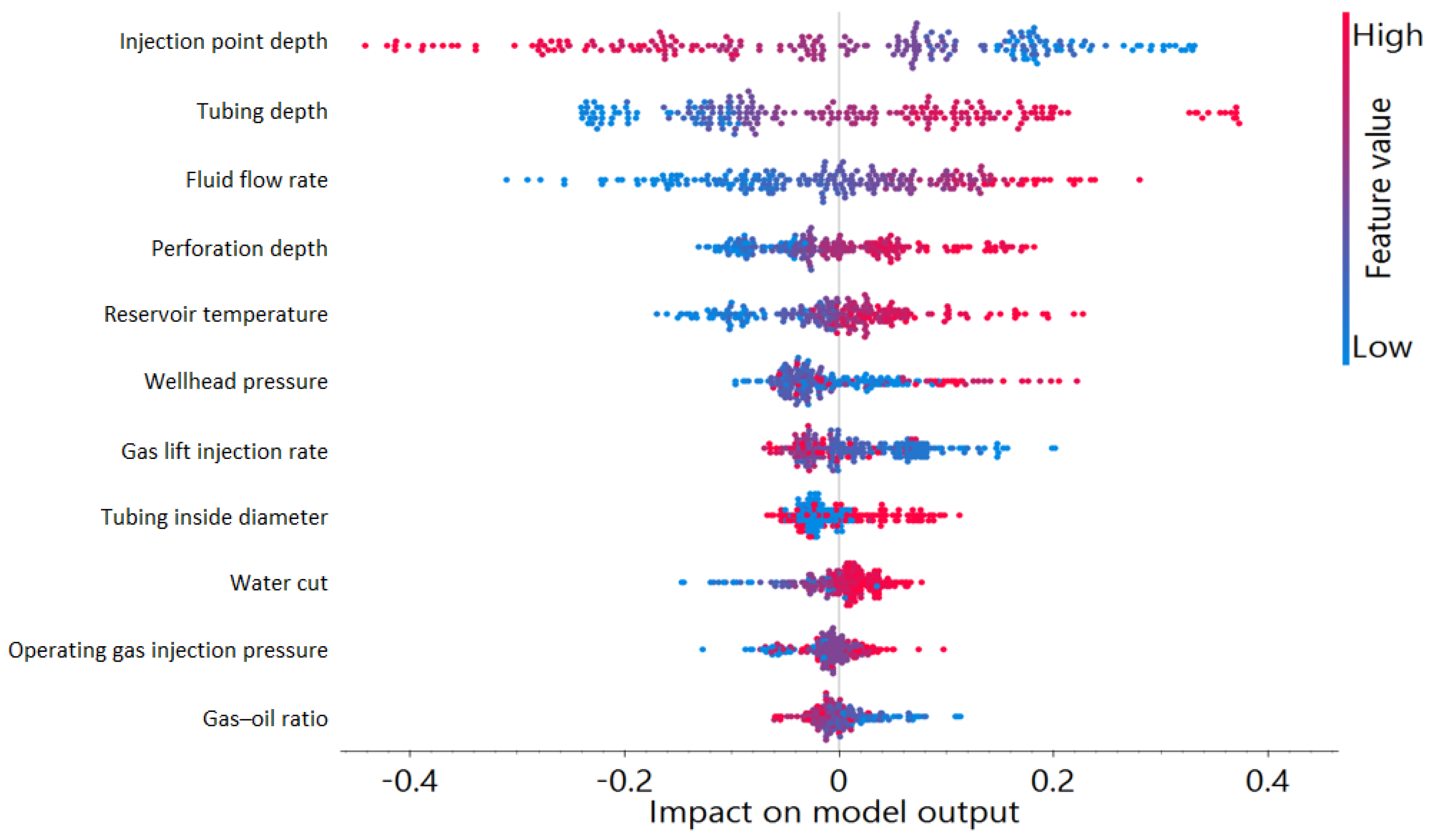
2.2. Feature Ranking

Relevant insights can be found in the data provided to machine learning models. These ML models require strong and meaningful connections between the inputs and the target for good outcomes. For this reason, it is important to understand the meaning of features linked to the correlation coefficient. The correlation coefficient was computed by employing Pearson’s and Spearman’s methods in this study. Pearson’s correlation coefficient is used to show the straight-line relationship between two uninterrupted variables, but it can be easily affected by outliers. Unlike Pearson’s, Spearman’s rank correlation coefficient (ρ) is not greatly affected by outliers and is suitable for non-normally distributed data that only show a monotonic relationship. Pearson’s r should be used for linear correlations only, whereas Spearman’s ρ is able to discover any trend, even if they are not straight lines. Both measures of correlation have values between −1 and +1. If two variables have a +1 value, then an increase in one is always matched by an increase in the other. If a perfect negative correlation exists, a value of −1 indicates that the two variables are always moving in opposite directions. A value of 0 indicates that there is no connection between the variables. Both measures are described by the Equations (1) and (2).

$$\mathrm{r}={\displaystyle \frac{\sum \left({\mathrm{X}}_{\mathrm{i}}-\overline{\mathrm{X}}\right)\left({\mathrm{Y}}_{\mathrm{i}}-\overline{\mathrm{Y}}\right)}{\sqrt{\sum {\left({\mathrm{X}}_{\mathrm{i}}-\overline{\mathrm{X}}\right)}^2}\cdot \sqrt{\sum {\left({\mathrm{Y}}_{\mathrm{i}}-\overline{\mathrm{Y}}\right)}^2}}}$$

(1)

Here,

• X_i and Y_i are the individual data points;
• $\overline{\mathrm{X}}$ and $\overline{\mathrm{Y}}$ are the means of X and Y;
• The numerator is the covariance of X and Y;
• The denominator is the product of their standard deviations.

$$\mathsf{\rho }=1-{\displaystyle \frac{6\sum {\mathrm{d}}_{\mathrm{i}}^2}{\mathrm{n}\left({\mathrm{n}}^2-1\right)}}$$

(2)

Here,

• d_i is the difference between the ranks of corresponding values in X and Y;
• n is the number of data points.

The graph in Figure 4 demonstrates the level of impact that input parameters such as WC, TID, GOR, FFR, RT, PD, TD, OGIP, WHP, GLIR, and IPD have on BHP. A strong correlation between BHP and WC, TID, and FFR is clear, while the rest of the parameters show moderate correlations.

Figure 5 displays a heat map that graphically displays how each parameter in the dataset is linked with the others based on the Pearson correlation matrix. There is a significant link between IPD and PD (95%), TD (95%), and RT (95%) because they show strong positive correlations. BHP has a positive and somewhat strong relationship with WC (0.52) and a weaker moderate one with FFR (0.28), but it tends to go negative with TID (−0.37). WHP, OGIP, and GLIR hardly correlate with most variables, which indicates they are independent. These insights clarify, with great importance, the parameters that influence gas lift systems and those that do not, helping explain their behaviors and predict how they will act.

In Figure 6, Spearman’s correlation between the features available in the data to predict the BHP is presented as a heatmap. There is a MODERATE positive link between WC, FFR, and BHP (0.5 for WC and 0.4 for FFR). Alternatively, the inverse relationship between TID (−0.5) and BHP is at the MODERATE level. Minimally direct influence can be found by analyzing features that are less connected to BHP.

2.3. Data Preprocessing

The process of data preprocessing in machine learning guarantees that the data are reliable and fitting for developing a model. Processing the data involves carrying out steps that make sure they are reliable, consistent, and accurate, which elevates the performance and quality of the model. The first step is to handle the missing data. We handled missing values by removing records with missing data and using the method of linear extrapolation from nearby points to estimate the gaps. We also detected unusual data points with the help of box plots and removed them, since they might interfere with the learning process. After that, data integration merges numerous data sources into one dataset.

Final processing includes standardization or normalization. This approach helps features of different scales to influence the model in a similar way. Regression machine learning models, which often use gradient descent, depend heavily on feature scales, as they impact the success of the model. Some popular methods of normalization are min–max scaling and z-score normalization. The study relied on the min–max scalar technique to process its data. When you have boundary information or favor knowing the exact range of the data, min–max scaling helps and is frequently used in k-NN and neural networks. Min–max scaling can be expressed in the following mathematical way:

$$X^{\prime }={\displaystyle \frac{X-X_{\mathrm{m}\mathrm{i}\mathrm{n}}}{X_{\mathrm{m}\mathrm{a}\mathrm{x}}-X_{\mathrm{m}\mathrm{i}\mathrm{n}}}}$$

(3)

where

• $X$ is the original value;
• $X_{\mathrm{m}\mathrm{i}\mathrm{n}}$ is the minimum value in the feature;
• $X_{\mathrm{m}\mathrm{a}\mathrm{x}}$ is the maximum value in the feature;
• $X^{\prime }$ is the normalized value (scaled to the range $\left[\mathrm{0,1}\right]$).

Lastly, the processed data were separated into 80% for use in training and 20% for testing. We chose this number to help ensure that the model has enough information for learning and enough unseen data to judge its ability to solve any new problem and notice overfitting.

2.4. Models Structure

2.4.1. Traditional Machine Learning and Neural Network-Based Approaches

Python 3.10.12 was used to set up and analyze fifteen models, and each model required the hyperparameter settings listed in

Table 2. Summary of machine learning and deep learning models with their hyperparameter configurations.

Model	Model Parameters
GB (scikit-learn)	Number of trees is 100 Learning rate is 0.1 Limit depth of individual trees is 3 Does not split subsets smaller than 10 The fraction of training instances is 0.8
EGB (xgboost)	Number of trees is 200 Learning rate is 0.05 Lambda (L2 regularization) is 1 Limit depth of individual trees is 6 Fraction of training instances is 0.8 Fraction of features for each tree is 0.8 Fraction of features for each level is 1 Fraction of features for each split is 0.8
EGB-RF (xgboost)	Number of trees is 200 Learning rate is 1 Lambda (L2 regularization) is 2 Limit depth of individual trees is 5 Fraction of training instances is 0.8 Fraction of features for each tree is 0.7 Fraction of features for each level is 1 Fraction of features for each split is 0.8
GB (catboost)	Number of trees is 100 Learning rate is 0.05 Lambda (L2 regularization) is 3 Limit depth of individual trees is 5 Fraction of features for each tree is 0.8
AdaBoost	The number of estimators is 100 Learning rate is 0.05 Boosting method is SAMME.R (Real boosting) Regression loss function is square
RF	Number of trees in the forest is 10 Number of attributes per split is 5 Limit depth of individual trees is 5 Do not split subsets smaller than 5
SVMs	SVM cost is 1 Regression loss epsilon: 0.1 Kernel type is linear Numerical tolerance: 0.001 Iteration limit is 1000
DT	Minimum instances in leaves are 15 Does not split subsets smaller than 7 Maximal tree depth is 10 The stopping point is at 95% of the majority
kNN (distance)	Number of nearest neighbors is 5 Metric is Euclidean Weight is by distance
KNN (uniform)	Number of nearest neighbors is 5 Metric is Euclidean Weight is uniform
LR	Fit intercept Regularization: Elastic Net regression Alpha: 10 L1:L2 mixing ratio: 0.5:0.5
NN (L-BFGS)	Sklearn’s Multi-layer Perceptron (MLP) algorithm Neurons per hidden layer are 50 Activation is ReLu Solver is L-BFGS-B Regularization: 0.01 Maximum iterations are 1000
NN (Adam)	Sklearn’s Multi-layer Perceptron (MLP) algorithm Neurons per hidden layer are 50 Activation is ReLu Solver is Adam Regularization: 0.01 Maximum iterations are 1000
NN (SGD)	Sklearn’s Multi-layer Perceptron (MLP) algorithm Neurons per hidden layer are 50 Activation is ReLu Solver is SGD Regularization: 0.01 Maximum iterations are 1000
SGD	Regression loss function is squared loss Regularization is Elastic Net Elastic Net mixing ratio is 0.5 Regularization strength is 0.001 Learning rate is constant Number of iterations is 1000

. Running the data through a multiple regression such as Neural Network-L-BFGS (NN-LBFGS), AdaBoost (ADAB), Extreme Gradient Boosting-XGBoost (XGB), Gradient Boosting-scikit-learn (GB-SKL), kNN by Distances (kNN-D), Gradient Boosting-CatBoost (GB-CB), Stochastic Gradient Descent (SGD), Support Vector Machine (SVM), Random Forest (RF), kNN Uniform (kNN-U), Neural Network-Adam (NN-Adam), Extreme Gradient Boosting Random Forest-XGBoost (XGB-RF), Linear Regression (LR), Decision Tree (DT), or Neural Network-SGD (NN-SGD) is necessary for this study. This process allows us to compare various models to see which performs the best on our data, as every model has certain advantages. Not every machine learning model is good for every kind of analytics; they are valuable for some and not for others. An example is that Gradient Boosting works best by reducing errors with each boost, leading to greater accuracy in situations with many complex and related variables, while Random Forest performs better at generalizing results by combining several Decision Trees with the ability to estimate how important each feature is and does well with high-dimensionality data. Support Vector Machines try to find the best division of cases based on kernel transformations, but their ways are not as simple and straightforward as those of Decision Trees. The quality of results stands out in K-Nearest Neighbors, since its training process is simple. Since linear relationships between variables can be addressed in a linear manner, Linear Regression suits this well and remains easy to understand while being efficient to compute. Neural networks can successfully discover the complex nonlinearity by the multi-layered structure with the ability of auto feature extraction. Stochastic Gradient Descent allows for optimizing the parameters of large datasets by performing small updates at a time. With all these algorithms available, we can choose the most suitable one for us in terms of how easy it is to interpret, the computational effort it requires, or how well it predicts results.

The behavior and functioning of machine learning models are defined by their model parameters. Some of the values they include are the number of trees, the learning rate, maximum tree depth, and regularization strength. Because of these parameters, a model learns from given data, avoids over- and underfitting, and easily applies to new situations. As an illustration, splitting trees into fewer levels or using regularization is useful to keep the model’s complexity low, but adjusting the learning rate can make the model settle down faster. SVM uses parameters regarding the number of nearest neighbors and kernel type to interpret its input data. Selecting different loss functions, types of activations, and optimizers for neural networks can make training more efficient and improve their accuracy in making predictions. To ensure the best performance, generalization, accuracy, and dependability, it is vital to be attentive to when and how to use these parameters.

Figure 7 displays the Pythagorean Forest visualization. All learned Decision Tree models from the RF model are shown in the Pythagorean Forest. The best trees are those with the shortest and darkest-colored branches. This means there are few things that divide the branches clearly. It is used to help understand the variety and detail in the Decision Trees included in an RF model. It helps determine the role that a single tree plays in the predictions and can point out any signs of overfitting or underfitting by noticing similarities in their structure or excessive depth across trees.

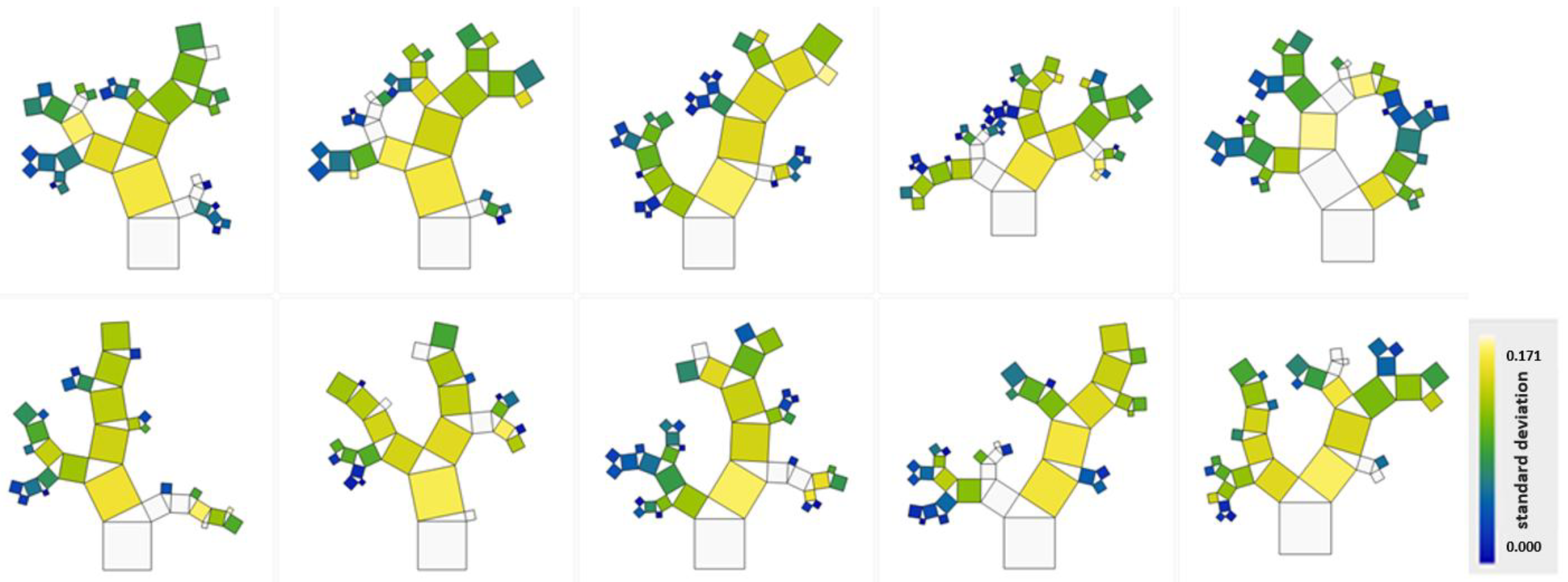
2.4.2. Genetic Programming-Based Symbolic Regression

Genetic programming-based symbolic regression (GPSR) is set as model number sixteen. It involves the system automatically finding ways to model the relationships in the data using the ideas behind natural selection and evolution. Python 3.10.12 (PySR package) was selected to develop the GPSR model, and

Table 3. Summary of symbolic regression models with their hyperparameter configurations.

Model	Model Parameters
GP-SR	Number of evolutionary iterations is 100 Maximum expression size is 20

shows the exact parameters that were chosen. Rather than fitting data to specific equations, GPSR learns new equations by using a group of candidate solutions that are chosen, crossed over, and mutated. With this strategy, GPSR can discover complex patterns that do not follow a specific pattern beforehand. A major point in favor of this model over traditional ML models is that it is easily interpreted. Using GPSR, the model provides simple equations rather than black-box predictions that people can read and use to understand what is happening beneath the predictions. It is also outstanding in the simulation of systems that function by laws that are not fully known, since both transparency and discovering the system’s structure matter most. Furthermore, thanks to its use of smaller datasets and ability to work with noise and irregular data, GPSR is very suitable in gas lift well modeling.

3. Results and Discussion

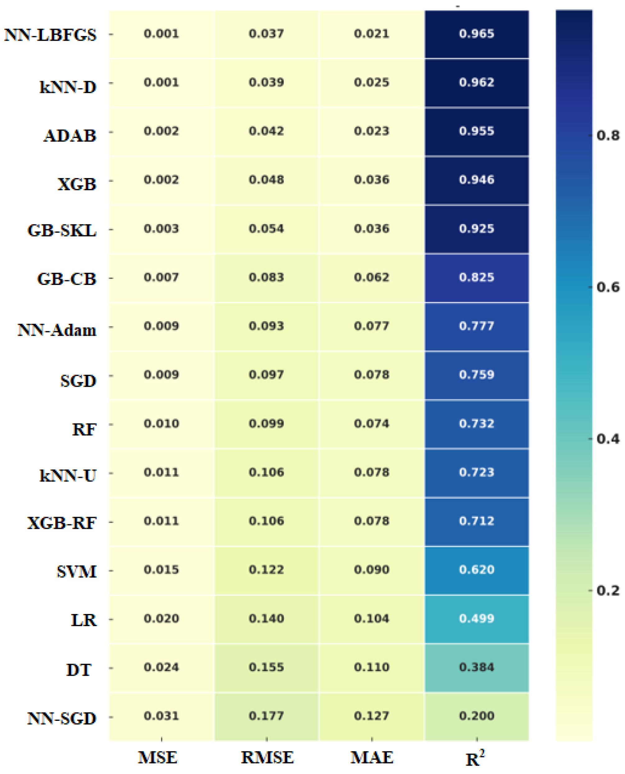
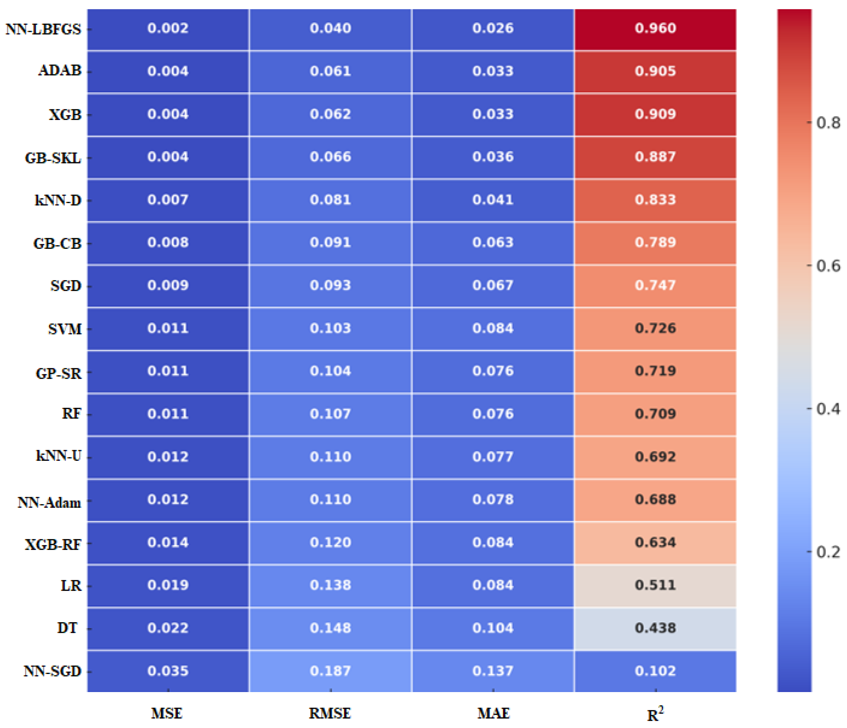
3.1. Model Results

The precision of the machine learning models can be observed in Figure 8 using the mean square error (MSE), root mean square error (RMSE), mean absolute error (MAE), and coefficient of determination (R2). As a result of the computations, we can tell how accurate each model is. An accurate model has a small error and a high R² level, while high errors and a low R² prove that the model performs poorly. That is why the NN (L-BFGS) model performs the best.

Figure 9 shows how the NN (L-BFGS) model predicted the BHP values compared to the BHP readings taken from the downhole gauges. Clusters of data on the diagonal line indicate that the predictions are highly accurate. You can see from the blue-to-yellow gradient that the model always works well, regardless of the pressure it is exposed to. The small scatter across the diagonal lines reflects that those predictions only slightly differ from the actual data. A smooth distribution of colors along the line helps prove that the model is both accurate and reliable for all pressure values.

The main variables influencing the BHP prediction, according to the NN (L-BFGS) model with SHAP (SHapley Additive exPlanations), are reported in Figure 10. The values from SHAP describe the impact of each feature on the outcome of the model so they can clarify the model’s behavior. The SHAP values, or the effects of each input (positive or negative), are found on the horizontal axis. Every observation is marked by a point that relies on the feature’s values (blue is the lowest, and red is the highest), and its position depends on the given SHAP value.

The importance of each parameter decreases as you move down, with the paramount one placed at the top. IPD, TD, and FFR appear to contribute the most to the differences in flowing BHP prediction, as they have the largest range of SHAP values going up and down. SHAP showed results that were not the same as those of the Spearman and Pearson models, as it focuses on the importance of features in a certain model, while these methods only consider areas where one feature affects another in a linear or single-directional manner. SHAP values are unlike correlation coefficients, which only restore the global linear or monotonic trend, and instead measure the local effect of each feature in individual predictions. This enables SHAP to detect nonlinear effects and interaction effects, for example, when the effect of a feature on BHP varies with other reservoir or operational parameters. So, SHAP identifies more complicated relationships and their significance compared to simple correlation statistics. SHAP values can help domain experts interpret the same results, learn how the model makes judgments, single out significant factors in the domain, and check the actual meaning of the parameters applied in the study.

GP-SR was used with the normalized data to produce models we could easily interpret. The chosen model (Equation (4)) delivered promising results when put to the test, having an MSE of 0.007, an RMSE of 0.085, an MAE of 0.068, and an R² of 0.802. Out of all the symbolic models shown in

Table 4. List of generated symbolic models alongside their loss and complexity evaluations.

Complexity	Loss	Equation
1	0.040771	0.3271417
3	0.028801	WC/2.23883
4	0.028639	Sin (WC) × 0.51090336
5	0.024993	${\displaystyle \frac{\mathrm{W}\mathrm{C}}{e^{\mathrm{c}\mathrm{o}\mathrm{s}\left(\mathrm{P}\mathrm{D}\right)}}}$
6	0.024519	WC/(cos (PD)/0.36379465)
7	0.019756	WC × (TD − IPD + 0.42867288)
8	0.016829	PD − ((WC × −0.37555227) + sin (IPD))
9	0.015375	(OGIP + WC) × (0.2983757 − (IPD − TD))
11	0.014491	(WC + OGIP) × (0.24029268 − (IPD − (PD × 1.095866)))
13	0.013551	((((FFR × 0.2097214) + 0.19042374) × (TD + WC)) + TD) − IPD
14	0.012628	(TD − ((FFR × WC) × −0.55305517)) − (cos (WHP) × (IPD/1.3678912))
15	0.010488	$(\sqrt{\mathrm{F}\mathrm{F}\mathrm{R}}\times 0.39444104+(\mathrm{T}\mathrm{D}-(\mathrm{I}\mathrm{P}\mathrm{D}\times \mathrm{c}\mathrm{o}\mathrm{s}(\mathrm{W}\mathrm{H}\mathrm{P}\left)\right)\left)\right)\times (\mathrm{W}\mathrm{C}+\mathrm{I}\mathrm{P}\mathrm{D})$
16	0.010348	(((WC + TD) × ((FFR × 0.2841561) + 0.13601056)) + TD) − (IPD × cos (WHP))
17	0.009773	$\left({\displaystyle \frac{\sqrt{\mathrm{F}\mathrm{F}\mathrm{R}\times 0.27031562}+(\mathrm{T}\mathrm{D}-(\mathrm{c}\mathrm{o}\mathrm{s}\left(\mathrm{W}\mathrm{H}\mathrm{P}\right)\times \mathrm{I}\mathrm{P}\mathrm{D}\left)\right)}{1.3074819}}\right)\times (\mathrm{W}\mathrm{C}+\mathrm{T}\mathrm{D})$
18	0.00901	$\left({\displaystyle \frac{\mathrm{T}\mathrm{D}-\left(\mathrm{c}\mathrm{o}\mathrm{s}\right(\sqrt{\mathrm{W}\mathrm{H}\mathrm{P}})\times \mathrm{I}\mathrm{P}\mathrm{D})}{1.3286747}}+\sqrt{\mathrm{F}\mathrm{F}\mathrm{R}\times 0.12889326}\right)\times (\mathrm{W}\mathrm{C}+\mathrm{P}\mathrm{D})$
19	0.008182	$(\mathrm{W}\mathrm{C}+\mathrm{T}\mathrm{D})\times \left({\displaystyle \frac{\mathrm{T}\mathrm{D}-\left(\mathrm{c}\mathrm{o}\mathrm{s}\right(\sqrt{\mathrm{W}\mathrm{H}\mathrm{P}})\times \mathrm{I}\mathrm{P}\mathrm{D})}{e^{\mathrm{G}\mathrm{L}\mathrm{I}\mathrm{R}}}}+\sqrt{\mathrm{F}\mathrm{F}\mathrm{R}\times 0.13287625}\right)$

, Equation (4) achieved the most suitable balance between accuracy and simplicity. The lowest loss it experienced was 0.010488, and its complexity was 15. Because symbolic models depend on both simplicity and being easy to read, some highly important features might not be included if they have little effect on the equation’s accuracy. In this case, we define complexity by the number of operations and variables needed in the model, which makes the model harder to understand. A better model fits the data, as its error or loss is lower. Thus, Equation (4) is the best model choice because it achieves good accuracy and is relatively simple.

$$(\sqrt{\mathrm{F}\mathrm{F}\mathrm{R}}\times 0.39444104+(\mathrm{T}\mathrm{D}-(\mathrm{I}\mathrm{P}\mathrm{D}\times \mathrm{c}\mathrm{o}\mathrm{s}(\mathrm{W}\mathrm{H}\mathrm{P}\left)\right)\left)\right)\times (\mathrm{W}\mathrm{C}+\mathrm{I}\mathrm{P}\mathrm{D})$$

(4)

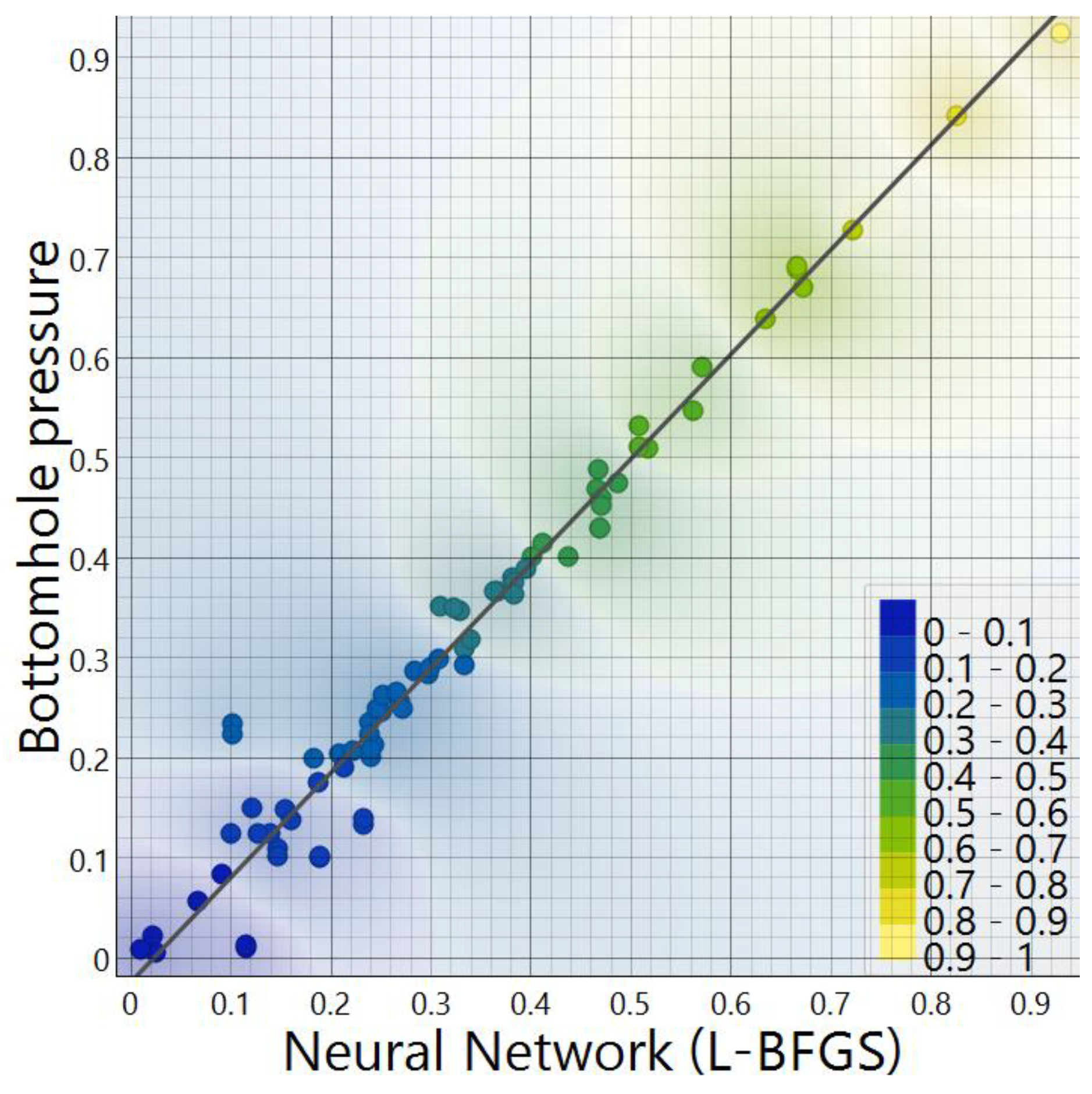
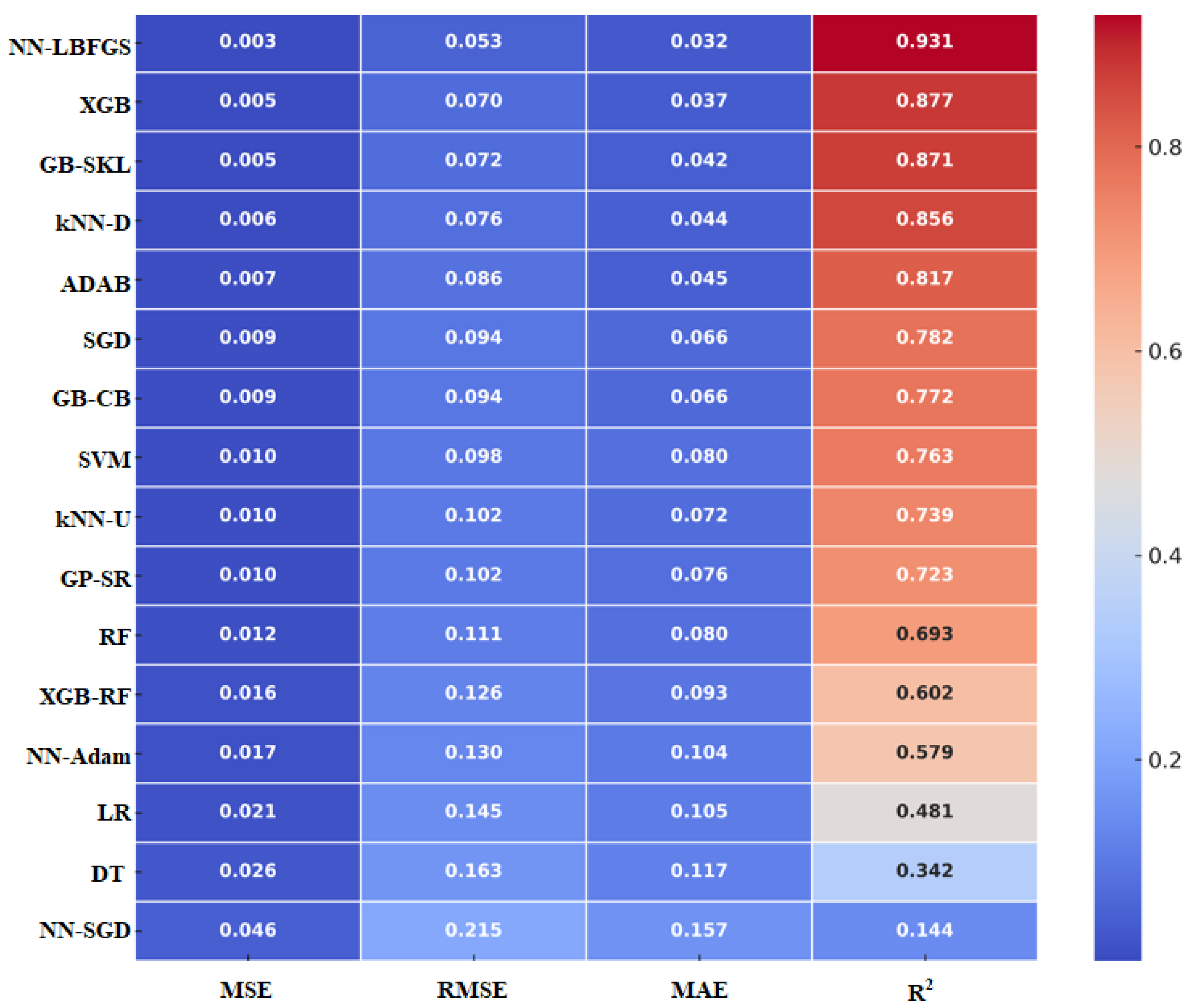
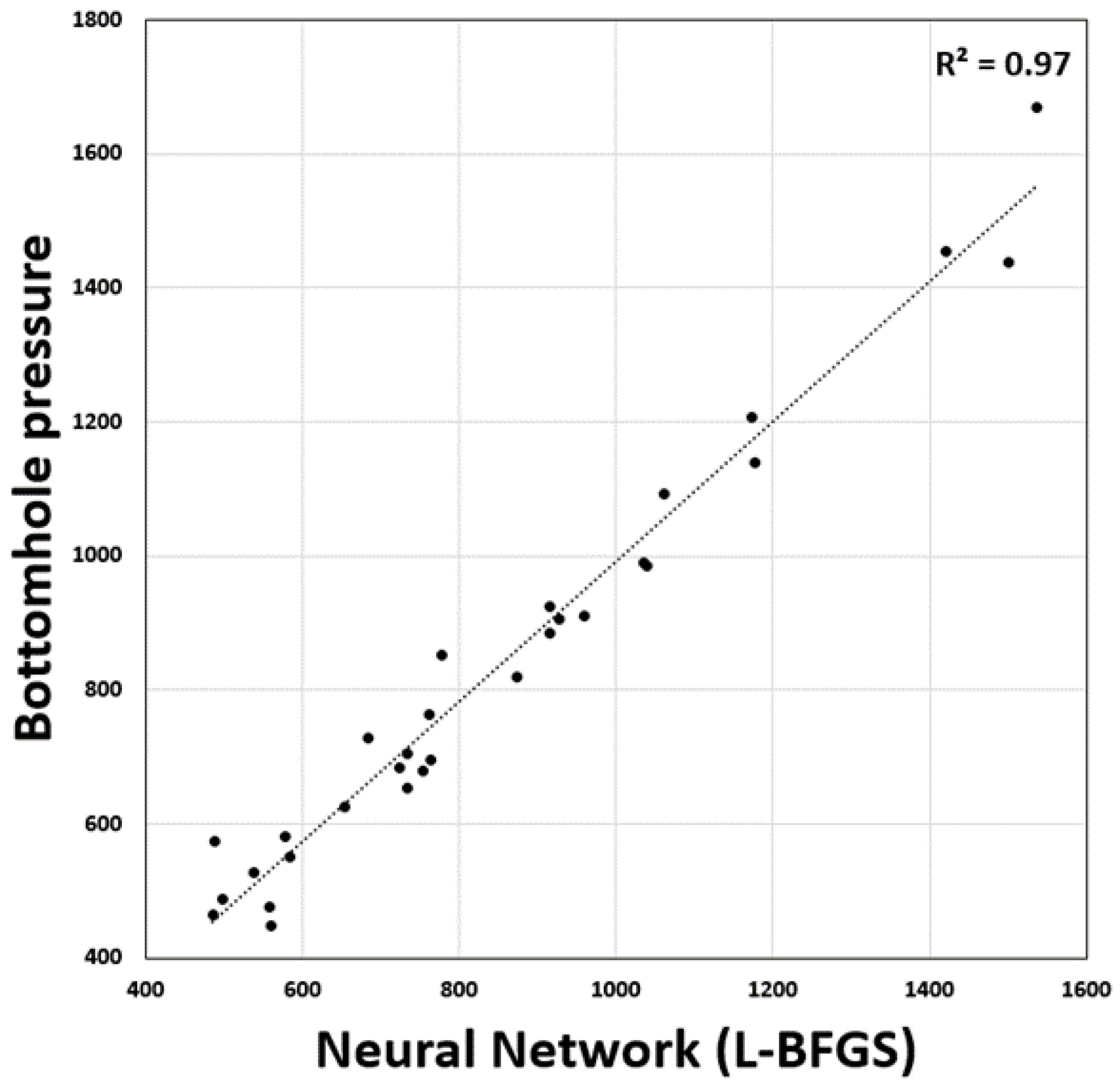
3.2. Model Testing and Validation

To determine the performances of the developed ML models, k-fold cross-validation testing is carried out along with random sampling techniques. The methods presented here give a set of procedures for validating the models and allow experts to agree on how effective they are. K-fold cross-validation is used in machine learning to split the data into K-folds, and only one-fold is tested at a time, with the rest being included in training. The process happens K times, and the metrics for prediction accuracy are averaged after each run. The technique is helpful in building models, since it gives a more dependable measure of how the model will work with fresh data. It prevents assessing an algorithm’s performance too positively by training and validating it with all the available data. It is also essential for choosing the best hyperparameters, selecting which model to apply, and lowering some types of bias. The cross-validation conducts training on nine folds and tests the regression model by using the only remaining fold (used as a test set). Figure 11 presents the outcome of the 10-fold cross-validation process. For each model, the outputs show the MSE, RMSE, MAE, and R².

In repeated random sampling cross-validation (RRSCV), the dataset is randomly split into training and testing subsets multiple times, and model performance is evaluated by averaging the results across these randomized iterations. Unlike the fixed splits in K-fold cross-validation, RRSCV uses multiple randomized splits to reduce the variation in its performance estimates. The main benefit is that with small data, this method makes better use of the data and results in more reliable findings of how the model would work on new data. It also works to identify if a model is overfitting and to adjust hyperparameters properly, helping select the best model when the data are unclear. Figure 12 displays the result obtained using the RRSCV technique after 10 iterations were performed. All the models have their MSE, RMSE, MAE, and R² presented with them. In K-fold and RRSCV evaluation, the neural network (L-BFGS) model obtains a higher accuracy than the other models.

3.3. Field Application

Blind dataset validation is the next validation process we will discuss. Blind dataset validation makes it possible to estimate the accuracy of a model in real life, as the new dataset is never used for training, tuning, or feature selection. This type of validation separates the test set up front, eliminating any risk of leaking data during a model’s development. While we can increase consistency using K-folds and reduce bias by sampling data several times, the truest and most accurate review comes from blind validation. For this reason, the developed NN (L-BFGS) model, which is the most accurate algorithm, was used with an independent set of data from 30 gas lift wells to estimate the flowing BHP during production. Descriptive statistics for each parameter are presented in

Table 5. Descriptive statistics for the dataset from 30 gas lift wells.

Parameter	Units	MIN	MAX	AVG	Median
Tubing inside diameter	inches	2.441	2.992	2.7165	2.7165
Tubing depth	ft	3200	10,318	6598.633	6220
Perforation depth	ft	3250	10,368	6686.3	6343
Wellhead pressure	psi	30	250	114.3333	100
Reservoir temperature	f	112.5	183.68	146.863	143.43
Gas–oil ratio	scf/stb	100	1500	582.5	500
Water cut	%	0	99	75.66667	90
Operating gas injection pressure	psi	800	1100	905	900
Gas lift injection rate	mmscf/d	0.4	0.9	0.52	0.5
Bottomhole pressure	psi	448	1661	800.2	745.5
Injection point depth	ft	2697	9253	5737.433	4799
Fluid flow rate	stb/d	50	1794	780.3667	734.5

.

The comparison between the BHP predicted by the developed NN (L-BFGS) algorithm and the memory gauge reading can be seen in Figure 13, and it is clear that the predictions match the measurements well with an R2 value of 0.97. Consequently, the system should make it possible to monitor the gas lift wells continuously and respond swiftly if an optimization decision is called for during production.

The use of the NN (L-BFGS) algorithm on 30 gas lift wells reveals that it can accurately forecast bottomhole pressure (BHP) per well. With this, it is now possible to constantly monitor and improve gas lift operations. Moreover, it is a cost-effective and reliable alternative to bottomhole gauges. In addition, these ML models are less likely to experience the accuracy issues seen with traditional methods based on physics, empirical correlations, or hybrid models. In complex fields such as those with big gas lift operations, involving thousands of wells operating concurrently, it is crucial to optimize operations as much as possible in real time.

3.4. Limitations of Machine Learning Models for BHP Prediction

Although these ML models for predicting BHP in gas lift wells are very accurate, they still have some limitations. They rely on substantial and well-prepared data and can work poorly with inaccurate, insufficient, or biased information. Unlike physics-based models, they are difficult to interpret, which makes the reasons for their behavior unclear. Changes in operational settings or well configurations may require frequent retraining. It is crucial to update ML models in a planned way when conditions in the field change, for example, retraining the model at scheduled times (e.g., three or six months) and keeping an eye on how accurately it predicts outputs to find out if any problems have developed. Lastly, model performance may be sensitive to hyperparameter tuning and data preprocessing techniques.

4. Conclusions and Future Work

It is based on the analysis of sixteen models that the NN (L-BFGS) model has shown the best results, with an R² of 0.965 and the minimal error metrics observed amongst all the algorithms tested (MSE = 0.001, RMSE = 0.037, and MAE = 0.021). These findings affirm its high predictability power in determining bottomhole pressure (BHP) using conventional well parameters. The same result was observed in k-fold cross-validation and repeated random sampling, which proved the model’s robustness and generalizability. In order to have a complete and objective comparison of performance, sixteen different machine learning models were trained on the same dataset. The method considers the variability in the strengths of the algorithms, deals with different data features, and provides the possibility to select the most accurate model to be used in the BHP prediction in complicated, actual gas lift conditions. By using SHAP analysis, it became clear that there are difficult, nonlinear relationships between injection point depth, tubing depth, fluid flow rate, and bottomhole pressure that other models cannot pick up.

The generalizability of the model was tested by blind testing on a separate dataset of 30 gas lift wells, where the model once again gave an R² of 0.97, which verified its strength and its applicability to the real world. Additionally, the symbolic regression model gave interpretable expressions with decent accuracy (R² = 0.80) that could be used as lightweight options when explainability is more important than accuracy. All the results prove the idea that a well-adjusted neural network can become an accurate, trusted, and cost-efficient substitute for the traditional BHP estimating techniques as well as downhole gauges.

More studies should focus on model generalizability by using various types of reservoirs, different operating situations, varying well structures, and several fluid types. If time-series data and dynamic operational changes are added, it would help improve accuracy and adaptability during real-time use. Additionally, applying physics-informed machine learning to symbolic regression might lead to code-based models that are easy to understand and yet perform well. Gathering global data from a wider range of field studies and building software tools for repeated training and deployment of the model will enhance opportunities for broad use. Overall, progress in ML will likely reshape optimization in gas lift operations, especially in complex mature fields such as those with huge gas lift operations including thousands of gas lift wells.

References

1. Su, S.J.; Ismail, A.M.; Al Daghar, K.; El-Jundi, O.; Mustapha, H. Maximizing the Value of Gas Lift for Efficient Field Development Plan Optimization Through Smart Gas Lift Optimization in a Giant Onshore Carbonate Oilfield. In Proceedings of the ADIPEC, Abu Dhabi, United Arab Emirates, 2 October 2023; p. D012S159R003. [Google Scholar] [CrossRef]
2. Moffett, R.E.; Seale, S.R. Real Gas Lift Optimization: An Alternative to Timer Based Intermittent Gas Lift. In Proceedings of the Abu Dhabi International Petroleum Exhibition & Conference, Abu Dhabi, United Arab Emirates, 13 November 2017; p. D021S048R004. [Google Scholar] [CrossRef]
3. Zhong, H.; Zhao, C.; Xu, Z.; Zheng, C. Economical Optimum Gas Allocation Model Considering Different Types of Gas-Lift Performance Curves. Energies 2022, 15, 6950. [Google Scholar] [CrossRef]
4. Khoshkbarchi, M.; Rahmanian, M.; Cordazzo, J.; Nghiem, L. Application of Mesh Adaptive Derivative-Free Optimization Technique for Gas-Lift Optimization in an Integrated Reservoirs, Wells, and Facilities Modeling Environment. In Proceedings of the SPE Canada Heavy Oil Conference, Virtual, 24 September 2020; p. D041S008R003. [Google Scholar] [CrossRef]
5. Suharto, M.A.; Risal, A.R.; Subandi, A.N.; Trjangganung, K.; Zain, A.M.; Ahnap, M.S. Maximizing Oil Production by Leveraging Python for Gas Lift Optimization Through Well Modelling. In Proceedings of the International Petroleum Technology Conference, Kuala Lumpur, Malaysia, 17 February 2025; p. D032S010R016. [Google Scholar] [CrossRef]
6. Mammadov, A.V.; Sultanova, A.V.; Mammadov, R.M. Grouping of Gas Lift Wells Based on their Interaction. In Proceedings of the SPE Caspian Technical Conference and Exhibition, Baku, Azerbaijan, 21 November 2023; p. D021S006R008. [Google Scholar] [CrossRef]
7. Yan, X.; Dong, J.; Niu, Z.; Liu, D.; Chen, A.; Gunay, A.; Cui, J.; Wang, Y.; Chen, J. Residual Oil Prediction According to Seismic Attributes and Oil Productivity Index Based on PCA and BPNN. In Proceedings of the Fourth International Meeting for Applied Geoscience & Energy, Houston, TX, USA, 26 August 2024; pp. 698–702. [Google Scholar] [CrossRef]
8. Amin, R.S.; Abdulwahab, I.M.; Rahman, N.M.A. Maximization of the Productivity Index Through Geometrical Optimization of Multi-Lateral Wells in Heterogeneous Reservoir System. In Proceedings of the International Petroleum Technology Conference, Dhahran, Saudi Arabia, 12 February 2024; p. D021S063R006. [Google Scholar] [CrossRef]
9. Alshobaky, A.M.; Abdal, W.S. Productivity Index in Horizontal Well. Malays. J. Ind. Technol. 2024, 8, 1–27. [Google Scholar] [CrossRef]
10. Abdullahi, B.A.; Ezeh, M.C. Production Optimization in Oil and Gas Wells: A Gated Recurrent Unit Approach to Bottom Hole Flowing Pressure Prediction. In Proceedings of the SPE Nigeria Annual International Conference and Exhibition, Lagos, Nigeria, 5 August 2024; p. D021S007R004. [Google Scholar] [CrossRef]
11. Mohammadpoor, M.; Shahbazi, K.h.; Torabi, F.; Qazvini, A.A. New Methodology for Prediction of Bottomhole Flowing Pressure in Vertical Multiphase Flow in Iranian Oil Fields Using Artificial Neural Networks (ANNs). In Proceedings of the SPE Latin American and Caribbean Petroleum Engineering Conference, Lima, Peru, 1 December 2010; p. SPE-139147-MS. [Google Scholar] [CrossRef]
12. Barrufet, M.A.; Rasool, A.; Aggour, M. Prediction of Bottomhole Flowing Pressures in Multiphase Systems Using a Thermodynamic Equation of State. In Proceedings of the SPE Production Operations Symposium, Oklahoma City, Oklahoma, 2 April 1995; p. SPE-29479-MS. [Google Scholar] [CrossRef]
13. Gunwant, D.; Kishore, N.; Gogoi, R.; Devshali, S.; Chanchalni, K.L.; Rajak, H.K.; Meena, S.K. Removal of Flow Instability Through the Use of Multiple Converging Gas Lift Ports (MCGLP) in Gas Lift Wells. In Proceedings of the SPE/IATMI Asia Pacific Oil & Gas Conference and Exhibition, Jakarta, Indonesia, 6 October 2023; p. D032S006R001. [Google Scholar] [CrossRef]
14. Popov, S.; Chernyshov, S.; Gladkikh, E. Experimental and Numerical Assessment of the Influence of Bottomhole Pressure Drawdown on Terrigenous Reservoir Permeability and Well Productivity. Fluid Dyn. Mater. Process. 2023, 19, 619–634. [Google Scholar] [CrossRef]
15. Gharieb, A.; Elshaafie, A.; Gabry, M.A.; Algarhy, A.; Elsawy, M.; Darraj, N. Exploring an Alternative Approach for Predicting Relative Permeability Curves from Production Data: A Comparative Analysis Employing Machine and Deep Learning Techniques. In Proceedings of the Offshore Technology Conference, Houston, TX, USA, 29 April 2024; p. D041S054R003. [Google Scholar] [CrossRef]
16. Campos, M.C.M.M.; Lima, M.L.; Teixeira, A.F.; Moreira, C.A.; Stender, A.S.; Von Meien, O.F.; Quaresma, B. Advanced Control for Gas-Lift Well Optimization. In Proceedings of the OTC Brasil, Rio de Janeiro, Brazil, 15 October 2017; p. D031S025R006. [Google Scholar] [CrossRef]
17. Garg, A.; Sharma, A.; Rajvanshi, S.; Suman, A.; Goswami, B.; Yadav, M.P.; Narayana, D.; Tiwary, R. Optimization of Gas Injection Network Using Genetic Algorithm: A Solution for Intermittent Gas Lift Wells. In Proceedings of the SPE Canadian Energy Technology Conference and Exhibition, Calgary, AL, Canada, 12 March 2024; p. D021S027R003. [Google Scholar] [CrossRef]
18. Masud, L.; Cortez, V.L.; Ottulich, M.A.; Valderrama, M.P.; Ghilardi, J.; Sanchez Graff, L.A.; Biondi, J.; Sapag, F. Gas Lift Optimization in Unconventional Wells—Vaca Muerta Case Study. In Proceedings of the SPE Argentina Exploration and Production of Unconventional Resources Symposium, Buenos Aires, Argentina, 20 March 2023; p. D011S004R002. [Google Scholar] [CrossRef]
19. Sajjad, F.; Chandra, S.; Wirawan, A.; Dewi Rahmawati, S.; Santoso, M.; Suganda, W. Computational Fluid Dynamics for Gas Lift Optimization in Highly Deviated Wells. In Proceedings of the SPE Annual Technical Conference and Exhibition, Dubai, United Arab Emirates, 15 September 2021; p. D021S032R002. [Google Scholar] [CrossRef]
20. Ali, A.M.; Negm, M.N.; Darwish, H.M.; Mansour, K.M. Strategic Modelling Approach for Optimizing and Troubleshooting Gas Lifted Wells: Monitoring, Modelling, Problems Identification and Solutions Recommendations. In Proceedings of the Gas & Oil Technology Showcase and Conference, Dubai, United Arab Emirates, 13 March 2023; p. D021S018R004. [Google Scholar] [CrossRef]
21. Ammar, M.; Abdulwarith, A.; Kareb, A.; Paker, D.M.; Dindoruk, B.; Ablil, W.; Altownisi, M.; Abid, E. Optimization of Gas Injection Well Productivity Through Integration of Modified Isochronal Test Including the Impact of Phase Behaviour: A Case Study on Coiled-Tubing Gas Lift for Al-Jurf Offshore Oil Field. In Proceedings of the SPE Annual Technical Conference and Exhibition, New Orleans, LA, USA, 20 September 2024; p. D021S022R007. [Google Scholar] [CrossRef]
22. Akinola, O.; Olufisayo, F.; Ebikeme, A.; Olumide, T.; Aluba, O.; Clement, C. Investigative Approaches to Troubleshooting and Remediating Sub-Optimal Gas Lift Performance in a Dual Completion Well. In Proceedings of the SPE Nigeria Annual International Conference and Exhibition, Lagos, Nigeria, 30 July 2023; p. D031S021R001. [Google Scholar] [CrossRef]
23. Elwan, M.; Davani, E.; Ghedan, S.G.; Mousa, H.; Kansao, R.; Surendra, M.; Deng, L.; Korish, M.; Shahin, E.; Ibrahim, M.; et al. Automated Well Production and Gas Lift System Diagnostics and Optimization Using Augmented AI Approach in a Complex Offshore Field. In Proceedings of the SPE Annual Technical Conference and Exhibition, Dubai, United Arab Emirates, 15 September 2021; p. D011S013R001. [Google Scholar] [CrossRef]
24. Algarhy, A.; Adel Gabry, M.; Farid Ibrahim, A.; Gharieb, A.; Darraj, N. Optimizing Development Strategies for Unconventional Reservoirs of Abu Roash Formation in the Western Desert of Egypt. In Proceedings of the The Unconventional Resources Technology Conference, Houston, TX, USA, 17 June 2024. [Google Scholar] [CrossRef]
25. Zalavadia, H.; Gokdemir, M.; Sinha, U.; Sankaran, S. Optimizing Artificial Lift Timing and Selection Using Reduced Physics Models. In Proceedings of the SPE Oklahoma City Oil and Gas Symposium, Oklahoma City, OK, USA, 17 April 2023; p. D021S003R002. [Google Scholar] [CrossRef]
26. Anuar, W.M.; Badawy, K.; Bakar, K.A.; Aznam, M.R.; Salahuddin, S.N.; Mail, M.; Bakar, A.H.; Trivedi, R.; Tri, N.V. Integrated Operations for Gas Lift Optimization: A Successful Story at Peninsular Malaysia Field. In Proceedings of the SPE Asia Pacific Oil and Gas Conference and Exhibition, Brisbane, Australia, 23 October 2018; p. D021S012R002. [Google Scholar] [CrossRef]
27. Chanlongsawaitkul, R. An Intelligent System to Recommend Appropriate Correlations for Vertical Multiphase Flow. Master’s Thesis, Chulalongkorn University, Bangkok, Thailand, 2006. [Google Scholar] [CrossRef]
28. Sun, H.; Luo, Q.; Xia, Z.; Li, Y.; Yu, Y. Bottomhole Pressure Prediction of Carbonate Reservoirs Using XGBoost. Processes 2024, 12, 125. [Google Scholar] [CrossRef]
29. Baryshnikov, E.S.; Kanin, E.A.; Osiptsov, A.A.; Vainshtein, A.L.; Burnaev, E.V.; Paderin, G.V.; Prutsakov, A.S.; Ternovenko, S.O. Adaptation of Steady-State Well Flow Model on Field Data for Calculating the Flowing Bottomhole Pressure. In Proceedings of the SPE Russian Petroleum Technology Conference, Virtual, 26 October 2020; p. D023S007R008. [Google Scholar] [CrossRef]
30. Cox, S.A.; Sutton, R.P.; Blasingame, T.A. Errors Introduced by Multiphase Flow Correlations on Production Analysis. In Proceedings of the SPE Annual Technical Conference and Exhibition, San Antonio, TX, USA, 24 September 2006; p. SPE-102488-MS. [Google Scholar] [CrossRef]
31. Campos, D.; Wayo, D.D.K.; De Santis, R.B.; Martyushev, D.A.; Yaseen, Z.M.; Duru, U.I.; Saporetti, C.M.; Goliatt, L. Evolutionary Automated Radial Basis Function Neural Network for Multiphase Flowing Bottom-Hole Pressure Prediction. Fuel 2024, 377, 132666. [Google Scholar] [CrossRef]
32. Agwu, O.E.; Alatefi, S.; Alkouh, A.; Azim, R. Artificial Intelligence Models for Flowing Bottomhole Pressure Estimation: State-of-the-Art and Proposed Future Research Directions. Int. J. Adv. Sci. Eng. Inf. Technol. 2024, 14, 1868–1879. [Google Scholar] [CrossRef]
33. Obeida, T.A.; Mosallam, Y.H.; Al Mehari, Y.S. Calculation of Flowing Bottomhole Pressure Constraint Based on Bubblepoint-Pressure-vs.-Depth Relationship. In Proceedings of the SPE Middle East Oil and Gas Show and Conference, Manama, Bahrain, 11 March 2007; p. SPE-104985-MS. [Google Scholar] [CrossRef]
34. Usov, E.V.; Ulyanov, V.N.; Butov, A.A.; Chuhno, V.I.; Lyhin, P.A. Modelling Multiphase Flows of Hydrocarbons in Gas-Condensate and Oil Wells. Math. Models Comput. Simul. 2020, 12, 1005–1013. [Google Scholar] [CrossRef]
35. Marfo, S.A.; Asante-Okyere, S.; Ziggah, Y.Y. A New Flowing Bottom Hole Pressure Prediction Model Using M5 Prime Decision Tree Approach. Model. Earth Syst. Environ. 2022, 8, 2065–2073. [Google Scholar] [CrossRef]
36. Chanchlani, K.; Sukanandan, J.; Devshali, S.; Kumar, V.; Kumar, A. Delineating and Decoding the Qualitative Interpretation of Gas Lift Instabilities in the Continuous Gas Lift Wells of Mehsana. In Proceedings of the International Petroleum Technology Conference, Kuala Lumpur, Malaysia, 17 February 2025; p. D022S006R008. [Google Scholar] [CrossRef]
37. Soni, D.K.; Mohammed Al Breiki, N. A Case Study of Well Integrity Challenges and Resolutions for the Gas Lift Appraisal Project: How 42 Gas Lift Wells Were Developed Post Mitigation of Well Integrity Challenges to Meet Double Barrier Compliance. In Proceedings of the SPE Middle East Artificial Lift Conference and Exhibition, Manama, Bahrain, 29 October 2024; p. D021S004R004. [Google Scholar] [CrossRef]
38. Orudjov, Y.A.; Dadash-zada, M.A.; Mamedov, F.K. Determination of the Critical Value of Bottomhole Pressure during Flow Well Operation. Azerbaijan Oil Ind. 2024, 23–26. [Google Scholar] [CrossRef]
39. Molinari, D.; Sankaran, S. Merging Physics and Data-Driven Methods for Field-Wide Bottomhole Pressure Estimation in Unconventional Wells. In Proceedings of the 9th Unconventional Resources Technology Conference, Houston, TX, USA, 26 July 2021. [Google Scholar] [CrossRef]
40. Barbosa, M.C.; Rodriguez, O.M.H. Drift-Flux Parameters for High-Viscous-Oil/Gas Two-Phase Upward Flow in a Large and Narrow Vertical and Inclined Annular Duct. J. Energy Resour. Technol. 2022, 144, 033004. [Google Scholar] [CrossRef]
41. Yin, B.; Pan, S.; Zhang, X.; Wang, Z.; Sun, B.; Liu, H.; Zhang, Q. Effect of Oil Viscosity on Flow Pattern Transition of Upward Gas-Oil Two-Phase Flow in Vertical Concentric Annulus. SPE J. 2022, 27, 3283–3296. [Google Scholar] [CrossRef]
42. Nagoo, A.S.; Vangolen, B.N. Will Gas Lifting in the Heel and Lateral Sections of Horizontal Wells Improve Lift Performance? The Multiphase Flow View. In Proceedings of the SPE Annual Technical Conference and Exhibition, Virtual, 19 October 2020; p. D041S053R007. [Google Scholar] [CrossRef]
43. Miranda-Lugo, P.J.; Barbosa, M.C.; Ortiz-Vidal, L.E.; Rodriguez, O.M.H. Efficiency of an Inverted-Shroud Gravitational Gas Separator: Effect of the Liquid Viscosity and Inclination. SPE J. 2023, 28, 429–445. [Google Scholar] [CrossRef]
44. Ualiyeva, G.; Pereyra, E.; Sarica, C. An Experimental Study on Two-Phase Downward Flow of Medium Viscosity Oil and Air. In Proceedings of the SPE Annual Technical Conference and Exhibition, Houston, TX, USA, 26 September 2022; p. D021S021R006. [Google Scholar] [CrossRef]
45. Xu, L.; Chen, J.; Cao, Z.; Zhang, W.; Xie, R.; Liu, X.; Hu, J. Identification of Oil–Water Flow Patterns in a Vertical Well Using a Dual-Ring Conductance Probe Array. IEEE Trans. Instrum. Meas. 2016, 65, 1249–1258. [Google Scholar] [CrossRef]
46. Wu, N.; Luo, C.; Liu, Y.; Li, N.; Xie, C.; Cao, G.; Ye, C.; Wang, H. Prediction of Liquid Holdup in Horizontal Gas Wells Based on Dimensionless Number Selection. J. Energy Resour. Technol. 2023, 145, 113001. [Google Scholar] [CrossRef]
47. Luo, C.; Wu, N.; Dong, S.; Liu, Y.; Ye, C.; Yang, J. Experimental and Modeling Studies on Pressure Gradient Prediction for Horizontal Gas Wells Based on Dimensionless Number Analysis. In Proceedings of the SPE Annual Technical Conference and Exhibition, Dubai, United Arab Emirates, 15 September 2021; p. D031S052R006. [Google Scholar] [CrossRef]
48. Liu, M.; Bai, B.; Li, X. A Unified Formula for Determination of Wellhead Pressure and Bottom-hole Pressure. Energy Procedia 2013, 37, 3291–3298. [Google Scholar] [CrossRef]
49. Xu, Z.; Wu, K.; Song, X.; Li, G.; Zhu, Z.; Pang, Z. A Unified Model to Predict Flowing Pressure and Temperature Distributions in Horizontal Wellbores for Different Energized Fracturing Fluids. In Proceedings of the 6th Unconventional Resources Technology Conference, Houston, TX, USA, 23 July 2018. [Google Scholar] [CrossRef]
50. AL-Dogail, A.S.; Gajbhiye, R.N.; AL-Naser, M.A.; Aldoulah, A.A.; Alshammari, H.Y.; Alnajim, A.A. Machine Learning Approach to Predict Pressure Drop of Multi-Phase Flow in Horizontal Pipe and Influence of Fluid Properties. In Proceedings of the Gas & Oil Technology Showcase and Conference, Dubai, United Arab Emirates, 13 March 2023; p. D011S011R002. [Google Scholar] [CrossRef]
51. Thabet, S.A.; Elhadidy, A.A.; Heikal, M.; Taman, A.; Yehia, T.A.; Elnaggar, H.; Mahmoud, O.; Helmy, A. Next-Gen Proppant Cleanout Operations: Machine Learning for Bottom-Hole Pressure Prediction. In Proceedings of the Mediterranean Offshore Conference, Alexandria, Egypt, 20 October 2024; p. D021S012R008. [Google Scholar] [CrossRef]
52. Asimiea, N.W.; Ebere, E.N. Using Machine Learning to Predict Permeability from Well Logs: A Comparative Study of Different Models. In Proceedings of the SPE Nigeria Annual International Conference and Exhibition, Lagos, Nigeria, 30 July 2023; p. D021S004R005. [Google Scholar] [CrossRef]
53. Safarov, A.; Iskandarov, V.; Solomonov, D. Application of Machine Learning Techniques for Rate of Penetration Prediction. In Proceedings of the SPE Annual Caspian Technical Conference, Nur-Sultan, Kazakhstan, 15 November 2022; p. D021S013R002. [Google Scholar] [CrossRef]
54. Fan, Z.; Chen, J.; Zhang, T.; Shi, N.; Zhang, W. Machine Learning for Formation Tightness Prediction and Mobility Prediction. In Proceedings of the SPE Annual Technical Conference and Exhibition, Dubai, United Arab Emirates, 15 September 2021; p. D011S018R005. [Google Scholar] [CrossRef]
55. Thabet, S.A.; El-Hadydy, A.A.; Gabry, M.A. Machine Learning Models to Predict Pressure at a Coiled Tubing Nozzle’s Outlet During Nitrogen Lifting. In Proceedings of the SPE/ICoTA Well Intervention Conference and Exhibition, The Woodlands, TX, USA, 12 March 2024; p. D021S013R003. [Google Scholar] [CrossRef]
56. Mukherjee, T.; Burgett, T.; Ghanchi, T.; Donegan, C.; Ward, T. Predicting Gas Production Using Machine Learning Methods: A Case Study. In Proceedings of the SEG Technical Program Expanded Abstracts 2019, San Antonio, TX, USA, 15 September 2019; pp. 2248–2252. [Google Scholar] [CrossRef]
57. Al Shehri, F.H.; Gryzlov, A.; Al Tayyar, T.; Arsalan, M. Utilizing Machine Learning Methods to Estimate Flowing Bottom-Hole Pressure in Unconventional Gas Condensate Tight Sand Fractured Wells in Saudi Arabia. In Proceedings of the SPE Russian Petroleum Technology Conference, Virtual, 26 October 2020; p. D043S032R002. [Google Scholar] [CrossRef]
58. Nashed, S.; Moghanloo, R. Replacing Gauges with Algorithms: Predicting Bottomhole Pressure in Hydraulic Fracturing Using Advanced Machine Learning. Eng 2025, 6, 73. [Google Scholar] [CrossRef]
59. Gabry, M.A.; Ali, A.G.; Elsawy, M.S. Application of Machine Learning Model for Estimating the Geomechanical Rock Properties Using Conventional Well Logging Data. In Proceedings of the Offshore Technology Conference, OTC, Houston, TX, USA, 24 April 2023; p. D021S028R004. [Google Scholar] [CrossRef]
60. El Khouly, I.; Sabet, A.; El-Fattah, M.A.A.; Bulatnikov, M. Integration Between Different Hydraulic Fracturing Techniques and Machine Learning in Optimizing and Evaluating Hydraulic Fracturing Treatment. In Proceedings of the International Petroleum Technology Conference, Dhahran, Saudi Arabia, 12 February 2024; p. D021S084R003. [Google Scholar] [CrossRef]
61. Zhuang, X.; Liu, Y.; Hu, Y.; Guo, H.; Nguyen, B.H. Prediction of Rock Fracture Pressure in Hydraulic Fracturing with Interpretable Machine Learning and Mechanical Specific Energy Theory. Rock Mech. Bull. 2025, 4, 100173. [Google Scholar] [CrossRef]
62. Yang, C.; Xu, C.; Ma, Y.; Qu, B.; Liang, Y.; Xu, Y.; Xiao, L.; Sheng, Z.; Fan, Z.; Zhang, X. A Novel Paradigm for Parameter Optimization of Hydraulic Fracturing Using Machine Learning and Large Language Model. Int. J. Adv. Comput. Sci. Appl. 2025, 16. [Google Scholar] [CrossRef]
63. Gharieb, A.; Gabry, M.A.; Soliman, M.Y. The Role of Personalized Generative AI in Advancing Petroleum Engineering and Energy Industry: A Roadmap to Secure and Cost-Efficient Knowledge Integration: A Case Study. In Proceedings of the SPE Annual Technical Conference and Exhibition, New Orleans, LA, USA, 20 September 2024; p. D011S007R002. [Google Scholar] [CrossRef]
64. Thabet, S.; Elhadidy, A.; Elshielh, M.; Taman, A.; Helmy, A.; Elnaggar, H.; Yehia, T. Machine Learning Models to Predict Total Skin Factor in Perforated Wells. In Proceedings of the SPE Western Regional Meeting, Palo Alto, CA, USA, 9 April 2024; p. D011S004R007. [Google Scholar] [CrossRef]
65. Ugoyah, J.C.; Ajienka, J.A.; Wachikwu-Elechi, V.U.; Ikiensikimama, S.S. Prediction of Scale Precipitation by Modelling its Thermodynamic Properties using Machine Learning Engineering. In Proceedings of the SPE Nigeria Annual International Conference and Exhibition, Lagos, Nigeria, 1 August 2022; p. D021S007R005. [Google Scholar] [CrossRef]
66. Carpenter, C. Decision Tree Regressions Estimate Liquid Holdup in Two-Phase Gas/Liquid Flows. J. Pet. Technol. 2021, 73, 75–76. [Google Scholar] [CrossRef]
67. Thabet, S.; Zidan, H.; Elhadidy, A.; Taman, A.; Helmy, A.; Elnaggar, H.; Yehia, T. Machine Learning Models to Predict Production Rate of Sucker Rod Pump Wells. In Proceedings of the SPE Western Regional Meeting, Palo Alto, CA, USA, 9 April 2024; p. D011S004R008. [Google Scholar] [CrossRef]
68. Musorina, A.D.; Ishimbayev, G.S. Optimization of the Reservoir Management System and the ESP Operation Control Process by Means of Machine Learning on the Oilfields of Salym Petroleum Development NV. In Proceedings of the SPE Russian Petroleum Technology Conference, Virtual, 12 October 2021; p. D021S006R004. [Google Scholar] [CrossRef]
69. Tan, C.; Chua, A.; Muniandy, S.; Lee, H.; Chai, P. Optimization of Inflow Control Device Completion Design Using Metaheuristic Algorithms and Supervised Machine Learning Surrogate. In Proceedings of the International Petroleum Technology Conference, Kuala Lumpur, Malaysia, 17 February 2025; p. D012S001R007. [Google Scholar] [CrossRef]
70. Leem, J.; Mazeli, A.H.; Musa, I.H.; Che Yusoff, M.F. Data Analytics and Machine Learning Predictive Modeling for Unconventional Reservoir Performance Utilizing Geoengineering and Completion Data: Sweet Spot Identification and Completion Design Optimization. In Proceedings of the ADIPEC, Abu Dhabi, United Arab Emirates, 31 October 2022; p. D021S062R002. [Google Scholar] [CrossRef]
71. Nashed, S.; Lnu, S.; Guezei, A.; Ejehu, O.; Moghanloo, R. Downhole Camera Runs Validate the Capability of Machine Learning Models to Accurately Predict Perforation Entry Hole Diameter. Energies 2024, 17, 5558. [Google Scholar] [CrossRef]
72. Halliburton; Chen, S.; Shao, W.; Halliburton; Sheng, H.; Halliburton; Kwak, H.; Aramco, S. Use of Symbolic Regression for Developing Petrophysical Interpretation Models. In Proceedings of the SPWLA 63rd Annual Symposium Transactions, Stavanger, Norway, 1 March 2022. [Google Scholar] [CrossRef]
73. Abdusalamov, R.; Hillgärtner, M.; Itskov, M. Automatic Generation of Interpretable Hyperelastic Material Models by Symbolic Regression. Int. J. Numer. Methods Eng. 2023, 124, 2093–2104. [Google Scholar] [CrossRef]
74. Latrach, A.; Malki, M.L.; Morales, M.; Mehana, M.; Rabiei, M. A Critical Review of Physics-Informed Machine Learning Applications in Subsurface Energy Systems. Geoenergy Sci. Eng. 2024, 239, 212938. [Google Scholar] [CrossRef]
75. Khassaf, A.K.; Al-hameed, Z.M.; Al-Mohammedawi, N.R.; Al-Mudhafar, W.J.; Wood, D.A.; Abbas, M.A.; Ameur-Zaimeche, O.; Alsubaih, A.A. Physics-Informed Machine Learning for Enhanced Permeability Prediction in Heterogeneous Carbonate Reservoirs. In Proceedings of the Offshore Technology Conference, Houston, TX, USA, 28 April 2025; p. D041S049R004. [Google Scholar] [CrossRef]
76. Gladchenko, E.S.; Illarionov, E.A.; Orlov, D.M.; Koroteev, D.A. Physics-Informed Neural Networks and Capacitance-Resistance Model: Fast and Accurate Oil and Water Production Forecast Using End-to-End Architecture. In Proceedings of the SPE Symposium Leveraging Artificial Intelligence to Shape the Future of the Energy Industry, Al Khobar, Saudi Arabia, 19 January 2023; p. D021S004R001. [Google Scholar] [CrossRef]
77. Abdulwarith, A.; Ammar, M.; Kakadjian, S.; McLaughlin, N.; Dindoruk, B. A Hybrid Physics Augmented Predictive Model for Friction Pressure Loss in Hydraulic Fracturing Process Based on Experimental and Field Data. In Proceedings of the Offshore Technology Conference, Houston, TX, USA, 15 April 2024; p. D031S030R006. [Google Scholar] [CrossRef]
78. Baki, S.; Dursun, S. Flowing Bottomhole Pressure Prediction with Machine Learning Algorithms for Horizontal Wells. In Proceedings of the SPE Annual Technical Conference and Exhibition, Houston, TX, USA, 26 September 2022; p. D021S038R004. [Google Scholar] [CrossRef]
79. Sami, N.A. Application of Machine Learning Algorithms to Predict Tubing Pressure in Intermittent Gas Lift Wells. Pet. Res. 2022, 7, 246–252. [Google Scholar] [CrossRef]
80. Rathnayake, S.; Rajora, A.; Firouzi, M. A Machine Learning-Based Predictive Model for Real-Time Monitoring of Flowing Bottom-Hole Pressure of Gas Wells. Fuel 2022, 317, 123524. [Google Scholar] [CrossRef]
81. Ahmadi, M.A.; Chen, Z. Machine Learning Models to Predict Bottom Hole Pressure in Multi-phase Flow in Vertical Oil Production Wells. Can. J. Chem. Eng. 2019, 97, 2928–2940. [Google Scholar] [CrossRef]
Figure 1. Overview of the methodological framework.
Fluids 10 00161 g001
Figure 2. Pair plot illustrating the relationships among all variables in the dataset used for BHP prediction.
Fluids 10 00161 g002
Figure 3. Violin plots illustrating the distribution of each parameter in the dataset.
Fluids 10 00161 g003
Figure 4. Ranking of input features according to their influence on BHP.
Fluids 10 00161 g004
Figure 5. Pearson correlation heatmap illustrating the linear relationships between features in the dataset applied for bottomhole pressure (BHP) prediction.
Fluids 10 00161 g005
Figure 6. Spearman correlation heatmap illustrating the linear relationships between features in the dataset applied for bottomhole pressure (BHP) prediction.
Fluids 10 00161 g006
Figure 7. The Pythagorean Forest visualizing all Decision Tree models constructed by the Random Forest algorithm.
Fluids 10 00161 g007
Figure 8. Performance evaluation heatmap of the implemented machine learning models.
Fluids 10 00161 g008
Figure 9. Normalized actual and predicted BHP comparison using neural network with L-BFGS optimizer.
Fluids 10 00161 g009
Figure 10. SHAP plot illustrating feature impact in the neural network with L-BFGS optimizer.
Fluids 10 00161 g010
Figure 11. K-fold cross-validation results across different models.
Fluids 10 00161 g011
Figure 12. Random sampling results across different models.
Fluids 10 00161 g012
Figure 13. Neural network (L-BFGS optimizer) prediction vs. actual BHP values across 30 gas lift wells.
Fluids 10 00161 g013