Abstract
This work—mixing an original experimental approach, as well as numerical simulations—proposes to study film boiling modes around a small nickel sphere. While dealing with a simple looking phenomenon that is found in many industrial processes and has been solved for basic quenching regimes, we focus on describing precisely how vapor formation and film thicknesses, as well as vapor bubble evacuation, affect cooling kinetics. As instrumenting small spheres may lead to experimental inaccuracies, we optically captured, using a high-speed camera, the vapor film thickness at mid height, the vapor bubble volume, and the bubble detachment frequency, along with the heat flux. More precisely, an estimation of the instant sphere temperature, in different conditions, was obtained through cooling time measurement before the end of the film boiling mode, subsequently facilitating heat flux evaluation. We encountered a nearly linear decrease in both the vapor film thickness and vapor bubble volume as the sphere temperature decreased. Notably, the detachment frequency remained constant across the whole temperature range. The estimation of the heat fluxes confirmed the prevalence of conduction as the primary heat transfer mode; a major portion of the energy was spent increasing the liquid temperature. The results were then compared to finite element simulations using an in-house multiphysics solver, including thermic phase changes (liquid to vapor) and their hydrodynamics, and we also captured the interfaces. While presenting a challenge due to the contrast in densities and viscosities between phases, the importance of the small circulations along them, which improve the heat removal in the liquid phase, was highlighted; we also assessed the suitability of the model and the numerical code for the simulation of such quenching cases when subcooling in the vicinity of a saturation temperature.
1. Introduction
The study of boiling is interesting for many applications that require efficient heat exchanges. Most of the time, boiling is used as a substantial energy sink. The principal information that is needed is the heat transfer between the solid and the fluid. Theoretical models and empirical laws were developed to assess this quantity. In 1934, thanks to a heat wire plunged into a bath full of water, Nukiyama [1] was the first to describe all the different modes of boiling by plotting heat fluxes versus temperature. Nucleation, transition boiling, and film boiling were observed. Then, a great deal of experiments in various fluids and conditions were made to enhance the comprehension of each mode. Pioneer works [2,3,4,5,6,7] and more recently [8,9] have proposed different correlations based on physical arguments in order to estimate heat flux laws. Some analytic models have also been proposed [10]. All of these works are very interesting and provide analytical laws. However, their precision remains limited when confronted by industrial configurations as they are often case-dependent.
The case of the film boiling mode is interesting in the configuration of quenching in liquid quenchants, where boiling modes are generally not fully controlled. Different quenching techniques exist. The more gentle ones use forced convection of neutral gases, such as nitrogen. More vigorous ones use liquid quenchants, such as oil or even water. Metallic parts are either disposed on grids plunged inside a still pool, or they are dropped by gravity and collected at the bottom. Forced convection can also be employed to further improve cooling speed by removing the vapor from the surface of the metallic part (see [11,12] for more information on the techniques and challenges regarding the quenching process). In quenching configurations with liquids whose vaporization temperatures are below the initial metallic part temperature, the temperature is usually higher than the Leidenfrost temperature, and the temperature there is above the vapor film, which entirely covers the solid surface. This determines the first steps of cooling during quenching, and it is thus an important mode to understand. The vapor film is, in reality, never really stable, and interface waves exist whatever the orientation of the heater. A pure conduction model in the vapor film is usually considered as a first estimation of the film boiling heat transfer. Scholars have showed that this estimation underestimates the heat flux by a factor of 25% for vertical film boiling [13]. This demonstrates that the convection inside the film plays a role, but its influence is moderate when compared to conduction. The vapor film thickness is then a key parameter to evaluate as it is directly linked with conductive fluxes.
For horizontal film boiling, Berenson formulated a theory based on Rayleigh Taylor instabilities, which yields a heat flux proportional to the overheating raised to the power of [3]. Klimenko extended these notions [14], introducing analogous considerations but also incorporated a finite vapor film thickness into the Rayleigh–Taylor instability framework. This modification gives rise to a distinct heat flux scaling, whereby the overheating influences the power of .
For vertical film boiling, boundary layer theories with pure conduction inside the vapor film have been developed for saturated conditions [10], both with subcooling [13,15,16,17,18,19] and with forced convection [9,20]. They predicted a film thickness that scales with the height to the power of , and this leads to a heat flux that scales with the height to the power . These models are interesting for a first approach. However, their reliability is limited as they are based on very simplified scenarios.
Furthermore, the mean film thickness is not a convenient parameter as it is not necessarily an increasing function of the heat flux [21]. Kelvin–Helmholtz instabilities are generally present at the liquid vapor interface. These waves create very small film thickness that drastically improve the heat transfers. Meduri et al. [9], inspired by Berenson’s model for horizontal configuration, suggested a correlation to account for these instabilities, which exhibited a scaling behavior with an overheating exponent of . Subcooling and forced convection were also taken into account as multiplicative factors as they happen to be important factors of the heat transfer magnitude. Honda et al. [22] applied this vision in the configuration of film boiling around a sphere. Their combination of the resolutions of an integrated form of the boundary layer equation in the vapor and of a wave equation in the liquid leads to a more accurate estimation of the temperature profiles and heat fluxes over the sphere.
In addition to the solid temperature, the control parameters of the film boiling mode around an immersed solid are its material properties, its geometry, as well as the subcooling and the fluid characteristics. The Leidenfrost temperature is also influenced by factors such as wettability and surface roughness. The decision was made to narrow the scope of this study to examine the impact of solid temperature and subcooling.
Regarding the temperature of the liquid that is away from the heater subcooling, its influence is studied by the consideration of the subcooling . Large subcooling tends to increase the heat flux, whatever the boiling mode. This is not surprising as the liquid is expected to consume a part of the heat delivered by the heater. However the larger impact lies on the values of the heat flux and the temperature at the minimum heat flux (MHF), which increase according to [18]. In the context of quenching, this implies that the lower the bath temperature, the quicker the vapor film rupture occurs. For example, in the experiment of Ebrahim et al. [23], where an Inconel-600 cylinder was quenched, the overheating at which the vapor film broke increased from 250 to 450 K between the subcooling of 2 to . This observation has been confirmed by other authors [19,24], and Ikkene et al. [25] have reported Leidenfrost temperatures above 800 °C for very high subcoolings (). Jouhara et al. [19] observed that the vapor film breakage nature was different depending on the subcooling. Wetting front propagation occurred exclusively under moderate subcooling conditions. In instances of exceptionally high subcooling, a rapid and explosive wetting phenomenon was observed, leading to instantaneous wetting of the entire heater surface.
The diversity of the mechanisms involved in boiling leads us to narrow the scope of our work to an initial benchmark. The reason behind this approach is to avoid tackling the full complexity of boiling at first and then capturing some fundamental features to be validated. Consequently, a choice was made to experimentally study the quenching of a small nickel sphere that was 1 cm diameter in water. Such a small scale allows for enhanced precision in describing the interface. Additionally, it helps in sustaining the film boiling mode through capillary forces. Moreover, the spherical geometry does not present any sharp edges that offer preferential wetting points. Nickel was chosen as a material due to its large thermal diffusivity, which ensures temperature homogeneity; its large specific heat capacity, which ensures boiling lasts for a long time; a moderate oxidation phenomena at high temperatures under air; and because it does not melt at the maximum studied temperatures (). The majority of industrial processes that engage in boiling operations utilize water, making it the most extensively studied medium in boiling research. High bath temperatures were also considered to improve the vapor film lifetime. At such a small scale using nickel, the significant temperature gradients within the sphere were minimized. As a result, the assumption of a uniform temperature distribution remained valid, effectively sidestepping the intricate thermal variations within the solid material (with a Biot number reaching a maximum of approximately 0.2). The other advantages of nickel is that it is not subject to phase transformation on those temperature ranges. Finally, this choice was motivated by more practical experimental reasons as small scales involve lower energies that are easier to handle.
The quenching of small spheres have already been studied in the literature, and some conclusions are already known. Dhir et al. [18] studied the quenching of 19 and 24 mm spheres of various materials. They showed that the larger the subcooling, the higher the Leidenfrost temperature (the latter was measured between 200 and for low subcooling below ()). The associated heat fluxes before the vapor film collapse was around 5 × 10⁴ , and it was also improved with subcooling. They showed that the flux varied with a power of the temperature in the absence of subcooling and forced convection. Radiation effects were shown to represent, at most, 10% of the total heat flux. Finally they observed that the Leidenfrost temperature was sensitive to the surface condition that was modified by oxidation during the heating. Jouhara et al. [19] had the same conclusions with their study of different shapes of copper parts. The larger the sphere diameter, the higher the heat fluxes. They observed transient wetting phenomena with high frequency at the top of the spheres during film boiling. In both studies, the film boiling was turbulent for low subcooling, with mean vapor thicknesses of around mm at . Both authors confirmed that the temperature was mostly homogeneous and that the temperature variation was proportional to the heat fluxes (this was also shown by Burns et al. [26]). Other studies have provided measurements of vapor film thicknesses and arguments for Leidenfrost temperature prediction, as summarised by Honda et al. [22].
The aim of this work was to investigate sphere quenching experiments with different bath temperatures in order to capture the main features of such systems and to analyze them with physical arguments. Those arguments were challenged with the help of a numerical simulation. Given the challenging characteristics of a large density ratio, low viscosity in both media, and a large latent heat of vaporization, simulating the phenomenon becomes complex. To address this, a dedicated numerical framework carried out with an in-house stabilized finite element solver was used. This framework not only supports the validation of our physical interpretation, but it also assessed the suitability of the model and numerical code for simulation. This approach has never been performed in the literature according to the best of the authors’ knowledge, and it is expected to provide valuable insights into the comprehensive hydrodynamics of the system for subcoolings in the vicinity of .
2. Experimental Apparatus
2.1. System Components
The system mainly controlled by thermal effects was validated using a quenching experiment. The test sample consisted of a nickel sphere that had a 1 cm diameter (Table 1), and it was heated in a oven with a temperature control ranging from to . The water-filled bath for quenching was 30 cm long, 15 cm wide, and 20 cm deep; it was made of glass and thermal silicone; and it was subjected to atmospheric pressure heated with an immersed heater. An aluminum base was inserted into the bath to mechanically support the test sample. In order to ensure that the temperature was accurately measured, a thermocouple for water and an pyrometer for the sphere were used. A schematic description of the whole set up is presented in Figure 1.

Table 1.
Physical properties of the nickel sphere.
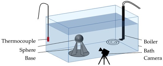
Figure 1.
Graphical scheme of the experimental test bench.
The camera set up included a NIKKOR VR 10–30 mm or a Nikon 105 mm f/2.8 AF Micro lens to capture images, and it was placed in front of the sphere at the same height. Opposite of the camera, a lighting system was set up to create a contrast. This way, the vapor film was easily identified from the liquid phase. Two types of shootings were used: a normal mode with real time images, and a high-speed camera mode with 400 pictures per seconds over 3 s.
2.2. Experimental Protocol
To ensure optimal reproducible tests in our experimentation, we paid attention to keeping the heating times and temperatures under control. Once we had succeeded in obtaining reproducible tests, we were able to carry out trials by varying the temperature of the oven and the temperature of the water.
Before each test, we turned on the oven and introduced the sphere once the desired temperature had been reached. During the oven heating phase, the thermal plunger was activated until the point of water boiling initiation. Once the oven had reached the designated temperature, the thermal plunger was turned off and the water naturally cooled down to the desired temperature. Afterward, the sphere’s temperature was measured with a pyrometer, and it was then quickly moved into the water bath using pliers. The chronometer started when the sphere was plunged and stopped when nucleate boiling started. To ensure comprehensive data capture, a series of high-frequency camera recordings were made throughout the boiling process. The last image was captured after post-boiling to provide a reference calibration for the post treatment. The resulting videos were then analyzed using MATLAB 2017a. It is pertinent to note that these measurements were exclusively conducted during the film boiling mode.
3. Experimental Method
3.1. Estimation of the Cooling Curve
Since no thermocouple was available to directly measure the sphere’s instantaneous temperature, an estimation of this temperature was conducted from the measurements of the quenching time. The idea was to consider that, whatever the initial condition, the sphere temperature could be recovered backward from the remaining time of the quench. This estimation was based on two assumptions.
The first was that the sphere temperature was uniform. This hypothesis can be validated by computing the diffusion time inside the sphere associated to half of its diameter :
where is the thermal diffusivity of the sphere whose value for nickel is 2.39 × 10⁻⁵ m2 s−1. This leads to a characteristic time , which is short compared to the experimental quenching times (from to ). Another way to evaluate this assumption is by considering the Biot number. In our configuration, it was approximately 10−2, indicating a significant impact of conductive effects within the solid. Consequently, it was reasonable to assume a uniform temperature distribution within the sphere. This assumption further enabled us to formulate the following energy conservation equation for the entire sphere:
where is the cooling rate of the sphere, is the mean heat flux around the sphere, is its surface, and its its volume.
The second hypothesis was that the cooling rate is solely dependent on the sphere temperature, bath temperature, and the inherent physical properties of the distinct phases. This entails that the previous states of the sphere do not influence its current behavior. Mathematically, this hypothesis leads to the existence of a monotonic function, denoted as f, which links the cooling rate and the current state as follows:
If we know this function f, we can integrate this equation to capture the current temperature in function of time t. The following strategy explains how to capture this function. The mathematical justification is first explained, then the practical method to assess the temperature on the basis of a heat transfer model is presented.
3.1.1. General Theory
Following this hypothesis, we can write the following:
Integrating this equation, there is a bijective function F that only depends on (as well as on material properties) and respects the following equality for every couple (,) and (,):
In other words at a given time t and for every couple (,) encountered by the cooling curve , the temperature reads as follows:
This property entails the existence of a master cooling curve: given a bath temperature, all cooling curves are linked together and follow the same path. For example, let us consider two cooling curves of initial temperature and , as shown in Figure 2. If we define the two associated cooling functions and , and if we define such that , then thanks to (6), we have the following:

Figure 2.
Graphical view of the master cooling curve. If the cooling rate is only a function of the temperature, then the two cooling curves of two different initial temperatures overlap on the same master curve.
If we synchronize the two cooling times (denoted as t and , such that when , or equivalently ), then we can establish , which is the two cooling curves coincide, forming a single master curve.
This curve is the same as the one obtained by plotting the initial temperature of the sphere versus the total cooling time , as shown in Figure 3. It can be easily estimated by several quenching tests with different initial temperatures. If we find the function , then the cooling curve of a given couple (,) reads as follows:
and
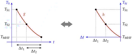
Figure 3.
Graphical view of the cooling curve and cooling time graph equivalency. The master cooling curve presented in Figure 2 can be obtained by plotting the initial temperature versus the cooling time.
Thus, if we can find a relationship between h and for any , we can obtain the function f.
To sum up, the following was performed:
- Several quenching tests were conducted at different initial sphere temperatures for a fixed bath temperature.
- The quenching time was measured for each experiment.
- This process resulted in an estimation of the function and, consequently, its derivative .
- A relationship was deduced.
3.1.2. Application in the Case of a Sphere
Dhir et al. [18] developed a boundary layer model of a vapor film around a sphere with subcooling. This resulted in a correlation between the cooling rate and the degree of overheating, yielding a power–law relationship of order . They challenged this model with experimental results, demonstrating favorable agreement. This result motivated us to write the following:
With this consideration, the problem can be simplified to finding the proportionality coefficient A. We noted , and we integrated (11) between and :
Thus, the function reads as follows:
Values of and A were then iteratively estimated to minimize the interpolation error with experimental values. The obtained parameters were used to assess the sphere temperature at any time t of the quench by integrating (11) between and :
Thanks to (2), the estimated cooling curve allowed us to estimate the heat flux noted .
3.2. Measurement of the Thermo-Hydrodynamic Quantities
The camera set up allowed us to observe the hydrodynamics of vapor. Three parameters were measured: the vapor film thickness at the mid height of the sphere , the volume of vapor bubbles that detached from the vapor film , and the frequency of bubbles created . To achieve this, we used a high-speed camera to capture 1200 frames in at different time steps of the experiments, with a resulting precision of , as stated in Section 3.3. According to the literature, liquid vapor interface movements that are captured during the film boiling mode are within the range of precision of this set up (see, for example, Vijaykumar et al. [17]), with wave film velocities of at most 1 m s−1 vertically and 0.05 m s−1 normal to the wall, as well as film boiling maximum thicknesses of, at most, 1 mm (see also Jouhara et al. [19] with minimum vapor film thicknesses of at most 1 mm).
Images of the vapor film around a hot nickel sphere immersed in water were captured with a Nikon camera at 60 fps. The post treatment of those images was conducted with a MATLAB code. The camera pictures were binarized to obtain matrices of 0 and 1 using the imbinarize MATLAB function. A very high contrast was required for this application. It was set up so that the liquid phase was identified with 0 (black pixels), whereas the vapor and solid phases were identified with 1 (white pixels). A correction was also implemented to fill the holes inside the vapor bubbles arising from the influence of light reflection effects. To do so, the imfill MATLAB function was used. This is explained in Figure 4.

Figure 4.
Example of the binarization of an experimental picture from a high-speed camera. The liquid phase was identified with black pixels, whereas the vapor and solid phases were identified in white. Reflection and refraction effects led to the misidentification of the vapor phase at the center of the bubbles, but this can be corrected with a filling function.
Once these preliminary steps were completed, the pixel size was converted to a physical length. This was achieved thanks to the pictures of the last video sequence. Indeed, in these last snapshots, the boiling was over and only the sphere remained with no vapor around. The scale could be computed with the measurement of the sphere diameter, which was known. The number of pixels of the sphere was counted, and, from this, we deduced the length of one pixel .
These pictures were analyzed in different ways to capture the desired quantities. Though the pictures only offered a 2D view of the experiment, the analysis was based on the assumption that the problem was axisymmetric. Thus, 3D estimations were extracted from this post-treatment. Moreover, thanks to the estimation of the cooling curve explained in last section, we could recover an estimation of the cooling rate . This was conducted thanks to the measurement of the difference of time between the snapshot and the time of collapse of the vapor film.
3.2.1. Vapor Film Thickness
The height of the sphere equator was obtained thanks to the snapshots of the sphere without boiling. At this height, the sphere and the vapor film on both sides were gathered in one horizontal line of white pixels (see Figure 5). Thus, the length of this line at this height corresponded to the sum of the diameter of the sphere and the two vapor film thicknesses (see Figure 5). Thanks to this consideration, and to the value of a pixel size , the current vapor film thickness was measured. This was performed for all 1200 pictures of every shot. The mean value was then computed as an estimation of .
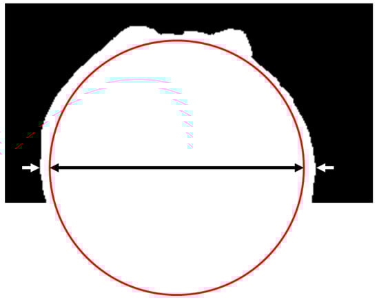
Figure 5.
Measurement of the vapor film thickness. The length of the line of white pixels at the height of the sphere equator was measured (delimited by the white arrows), and it corresponded to the sum of the diameter of the sphere (the black arrow) and the two vapor film thicknesses.
3.2.2. Vapor Bubble Volume
Under the assumption that the bubbles were axisymmetric, the revolution of the cross section measured was defined as the bubble volume. On each frame, we considered that each pixel line is a cylinder with a diameter that is the length of the line corrected by and whose height is . The sum of the infinitesimal cylinders of the bubble is an estimation of its volume. This estimation is described in Figure 6 and was conducted for all 1200 pictures of each video. We only considered the largest volume for each picture. However, the recovered volume was not constant. In fact, the development of the bubble resulted in an increase in volume before its detachment from the vapor film. Furthermore, condensation effects caused the bubble to shrink as it ascended. The volume variation resulting from those effect are represented in Figure 7.

Figure 6.
Axisymmetric 3D model of a vapor bubble recovered from a 2D binarized picture. The length of each line of white pixel is considered to be an infinitesimal cylinder. The sum of these cylinder represents an estimation of the bubble volume.

Figure 7.
Measurement of the vapor bubble volume and detachment frequency over a high-frequency snapshot. The measurement of a bubble varies in regard to the time required for the bubble formation process and condensation. However this variation is periodic. The period of this signal leads to the measurement of the detachment frequency. The addition of the amplitude of this frequency with the constant value of the signal leads to the bubble volume.
The volume of the sphere was then taken as the mean value of all the peaks of this quasi-periodic function (see Figure 7a). As the signal was close to being periodic with a single frequency, it could be decomposed by a constant (the mean of the signal) and a sinusoidal signal whose amplitude expresses the deviation from the mean. The volume of the bubble was, then, the sum of the constant with the amplitude of the sinusoid. By employing a Fast Fourier Transform, the signal was transformed from the time domain to the frequency domain. This transformation separated the signal into its constituent frequencies, enabling clearer identification of the dominant frequency components (see Figure 7b). Adding the amplitude of the first non-zero peak in the Fast Fourier Transform output to the volume mean value of the period enabled the estimation of the vapor bubble volume, which is denoted as .
3.2.3. Vapor Bubble Detachment Frequency
The period of the volume measurement signal was directly linked with the detachment frequency. The first non zero frequency was identified as the detachment frequency . This procedure was, however, tempered by a phenomenon that occurs at high sphere temperatures and at low subcooling, which is when the vaporization was strong. In this context, the bubbles were so large that some merged with the previous one. This lead to the measurements of doubled bubble volumes along with half detachment frequencies. These pathological cases were solved through manual correction.
3.2.4. Equivalent Heat Fluxes
The measurement of the vapor film thickness allowed us to recover an estimation of the heat fluxes at the surface of the sphere. Considering the pure conduction inside the vapor film, the associated heat flux read as follows:
where is the thermal conductivity of the vapor. This estimation was based on the assumption that the vapor film thickness at the equator of the sphere is a reliable value for the global vapor film thickness around the sphere. The vapor film model of [18] predicts a thickness that is close to be constant in the south hemisphere of the sphere. However, the area of detachment of the bubbles undergoes a great deal of perturbations and might deviate from this estimation.
The measurement of the vapor bubble volumes and detachment frequencies allowed us to estimate the energy used to vaporize the liquid. We defined an equivalent heat flux as follows:
where is the density of vapor, is the surface of the sphere, and is the latent heat in the vaporization of water. This estimation needs careful consideration as it overlooks the potential significant condensation effects occurring over the vapor film and during the bubble’s development.
3.3. Measurement Uncertainties
Regarding the bath temperature, the thermocouple was placed at one corner of the bath. Thus, the bath temperature inhomogeneities were not captured. Furthermore, at elevated temperatures, the bath temperature gradually declined by over 1 K/min, introducing a 1 K uncertainty in liquid temperature assessment.
Several uncertainties were noticed regarding the sphere temperature:
- Oven temperature inhomogeneity, up to , compromised the reliability of the oven temperature as an indicator. Proximity constraints limited pyrometer precision, yielding a uncertainty in measurements (thus, the pyrometer precision is not relevant here to define uncertainties).
- Sphere’s transfer from oven to bath caused temperature loss. Convective effects predicted by the Whitaker correlation [27] were negligible in our system. Radiation effects, with associated radiative heat flux , contributed at higher temperatures. Considering this radiative heat flux , the associated temperature drop was aroundat the highest temperature (900 °C), and a black body model led to a cooling rate of 10 K s−1. The sphere’s transfer took about , leading to a potential overestimation of . However the real emissivity of the nickel should be lower than 1. Another uncertainty was then considered to be conservative.
- A bath temperature variation caused a estimation fluctuation, magnifying temperature uncertainty.
- Conduction effects at the aluminum base contact point were considered negligible, primarily due to the minimal ratio between spike and sphere diameters. Despite this, their presence could potentially contribute to enhanced wetting and could, consequently, result in high .
- The spheres used for the experiments underwent oxidation during oven heating. This could be another potential source of error for the estimation of .
Regarding the uncertainties of the measurement deduced from optical visualization (film thickness, bubble volume. and bubbles detachment frequency), they were linked with the camera set up resolution. As two types of shootings were used (60 frames/s or 400 frames/s), temporal precision was, thus, about 17 ms and 2.5 ms, respectively. Spatially, precision depends on camera placement and image resolution (which is dropped in the high-speed mode). In our specific set up, it was typically /pixel for normal mode and /pixel for high-speed mode. As this latter mode was used for the measurements, this pixel’s translation to a physical distance of value defines the resolution of the cameras set up. While this influence may not be trivial, it is unlikely to substantially affect bubble volume estimations. However, a notable uncertainty arises from the inherent non-sphericity of the bubbles, i.e., a challenge in quantification. Our estimation indicates the potential for a significant 30% error due to this factor. Furthermore, the window frame occasionally truncated the edges of larger bubbles, introducing heightened uncertainty, which is particularly relevant at high overheating experiments. The frequency measurement stood out as highly reliable, and it was driven by consistent data periodicity. This was evidenced by the distinctive amplitude peaks recorded at the localized frequencies within the Fourier transform. The uncertainty was mostly due to the thickness of the peak overlapping with a small interval of frequencies of around .
We must mention the experiments conducted at low initial temperatures. We tried to directly estimate with such trials by considering the limit initial temperature at which the vapor film did not appear. However, it seemed that the hydrodynamical effects had an important impact on the vapor film stability. This instability occurred at temperatures higher than the expected threshold, leading to inconclusive results.
4. Experimental Results
4.1. Cooling Curve Estimation
We estimated the cooling curve with around twenty experimental points with initial temperatures ranging from to . Two water bath temperatures were considered (leading to a subcooling of and , respectively): and . The initial sphere temperatures versus the associated measured cooling times at a given water bath temperature are plotted in Figure 8. We also recall the interpolation function (13) we aimed for:

Figure 8.
Experimental measurements of the initial sphere temperature versus quenching time for the two bath temperatures. The fitting curves based on the boundary model are plotted.
Values of A and were iteratively determined to optimally match the two experimental curves. Error bars were estimated to account for the deviations in the measurements. The fitting curves are also depicted in Figure 8. The corresponding A and values are compiled in Table 2.
Table 2.
Experimental estimations of the Leidenfrost temperature and cooling rate coefficient.
The consistency of the values with the existing literature [18] is noteworthy. Dhir et al. observed a range of minimum film boiling temperatures () from 95 to 111 for a subcooling, as well as from 165 to 204 for a subcooling. In our study, we found to be during subcooling and during subcooling, thus being in the upper bounds of the values of [18] with experimental uncertainties. Variations of were usually around per Kelvin of subcooling, which is once again consistent with our estimation [23,28]. The values of A were also in the same order of magnitude as in [18], whose correlation led to a value of . The variation of heat flux from to subcooling was measured as around 5% in [18] compared to the 3% variation in this work deduced from the values of A.
Overall, the experimental data consistently align with the cooling rate model. The data scatter was assumed to be mainly due to the uncertainties on the bath temperature. A deviation of could substantially extend the quenching duration by several seconds. This impact was magnified in baths, where maintaining uniform temperatures near saturation levels becomes challenging. While the collective behavior should closely mirror the predicted trend, this variability also applies to individual quenching trials. The estimated temperature and cooling rate were notably influenced by the deviations arising from bath temperature uncertainty.
The order of magnitude of associated heat fluxes is around 1 × 10⁵ W m−2, which is consistent with the order of magnitude of heat fluxes in film boiling for large overheating. We also noticed that the cooling rate was improved by subcooling, which is consistent with observations in the literature [18,19]. But this improvement holds limited significance as there is a difference of only a few percentage points between the two cooling rates (see Figure 9). The most notable effect is the increase in , which aligns with the conclusions of Dhir et al. [18].

Figure 9.
Representation of the experimental cooling curves for the two bath temperatures. The cooling curves were close from each other, but the Leidenfrost temperature was significantly different. Pictures of some bubble regimes are plotted at the associated points. As expected, the hotter the sphere, the larger the bubbles, and the colder the bath, and the smaller the bubbles.
4.2. Qualitative Comments on the Camera Observations
Experiments were conducted using the camera set up at the consistent temperatures of and .
Initially, a diverse range of boiling modes were observed during the quench process with a predominant film boiling mode, as anticipated. Figure 10 depicts the quench progression at various time intervals and estimated temperatures, beginning at an initial temperature of with a bath temperature of . At first, a large amount of vapor forms, creating large bubbles that can eventually coalesce with the preceding ones. This results in a highly unstable, undulating interface, which is consistent with the observations of [29]. Over time, the vapor production decreases while ascending bubbles undergo condensation, rapidly vanishing after forming toward the end of the quench. For this initial temperature, these states lasted around . At certain points, bubble formation slows down and stops temporarily until wetting initiates. Wetting occurs all over the sphere at the same time, reaching the regime of explosive wetting described by Jouhara et al. [19]. Depending on the quenches, nucleated boiling follows immediately after wetting or after a few wetting iterations. However, there was no consistent pattern observed for these conditions. After this rapid transition boiling mode, an intense nucleate boiling phase began with a large quantity of vapor that was created within a short time. This phase continued for a few seconds before concluding with a brief period of partial nucleate boiling, ending the sphere’s cooling process.

Figure 10.
Snapshots at different times of the quenching of a sphere with a 98 bath temperature. Temperatures were estimated thanks to the cooling curve estimation, except for nucleation boiling, where they are postulated for illustration purposes. (a) At the beginning of the quench, a great deal of vapor is created, with bubbles that coalesce with the previous ones. The interface is very unstable and wavy. (b–f) Then, the vapor created reduces with time. Bubbles condensate when rising. The interface remains unstable and is wavy with a similar behavior. (g) At some points, the creation of bubbles slows and stops down until wetting starts. (h) Then, a violent nucleate boiling starts with a large quantity of vapor created in a short amount of time. (i) Partial nucleate boiling ends the cooling of the sphere. (j) Finally, the boiling stops and the sphere cools down with natural convection to the bath temperature.
From the observation of the vapor film and vapor bubble, the vapor velocity was estimated to be around −1. Considering the diameter of the sphere as a reference length, this led to a Reynolds number of 500. Flows inside the vapor were, thus, close to being laminar. However, the liquid–vapor interface exhibited notable undulations, which were characterized by phase velocities reaching −1, which is consistent with the measurements of [17], who obtained the same orders of magnitude. Normal velocities of the liquid–vapor interface were assumed to be comparable to the rate of wave development −1 over a characteristic distance of mm (order of magnitude of the wave amplitude), which is also consistent with the measurements of [17]. This resulted in a Reynolds number of approximately 100 within the liquid phase. The liquid phase was also mainly in a laminar regime but seemed to undergo important local recirculations close to the interface due to the vapor waves. This phenomenon is expected to contribute to the enhanced heat transfer by convection. Interestingly, the presence of these small-scale interface perturbations also demonstrates that surface tension is not the main factor of interface behavior.
It was difficult to precisely estimate whether transient wetting phenomena were frequent or not. Given that the measured wave amplitude surpassed the mean vapor film thickness, it is likely that the interactions between the liquid and solid surfaces occurred as demonstrated by [29].
The vapor bubbles shape were associated with a large Galilei number (∼104) and moderate Eötvös numbers (∼1), which are linked with asymetric bubbles that can evolve into doughnut-like or toroidal shaped bubbles (refer to [30] for more details). This is what was mostly observed for large bubbles at the high overheating temperatures when two bubbles interact (see Figure 10a). However, the condensation process might influence a great deal of their shapes as the bubble profiles turn into cap while decreasing in volume (refer to Figure 10f). This phenomenon is particularly pronounced under conditions of significant subcooling.
4.3. Quantitative Results
Five quenches were carried out with the camera set up, leading to five batches of measurements. The gathered data include measurements of the vapor film thickness at the sphere’s mid height , the volume of vapor bubbles detaching from the vapor film , and the frequency of bubble creation , and these measurements are plotted in Figure 11, Figure 12, and Figure 13, respectively.
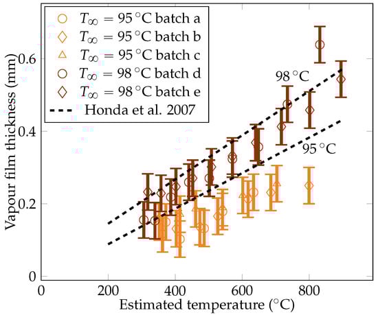
Figure 11.
Experimental measurements of the vapor film thicknesses at the equator of the sphere for liquid temperatures of and , compared with data of Honda et al. [22].

Figure 12.
Experimental measurements of the vapor bubble volumes for the liquid temperatures of and .

Figure 13.
Experimental measurements of the vapor bubble detachment frequency from the sphere for the liquid temperatures of and .
4.3.1. The Vapor Film Thickness
The metric decreases with temperature. The liquid horizontal heat flux was assumed to be stable. To maintain the stability of the vapor film, the decreasing temperature difference within the film must then be compensated by a decrease in the film thickness. This argument also explains the higher subcooling results that are produced in a thinner vapor film. The measurements were compared with the theoretical values predicted by Honda et al. [22]. The model was found to recover the proper order of magnitude of the film thickness, albeit with a small overestimation. The current measurements were being overestimated by only 10 to 30%, which is close to the experiment uncertainty and supports the validity of the experimental results.
4.3.2. The Volume of the Vapor Bubbles
The metric decreases with the sphere temperature. In fact, the lower the overheating, the more dominant the subcooling effects. These conditions entail stronger bubble condensation, which reduces their size as they develop. The order of magnitude of the bubble volumes were consistent with the measurements reported by Hosler et al. [31] for horizontal plates, with values of diameters of bubbles between 0.8 cm and 1.8 cm.
4.3.3. The Frequency of the Detachment of Bubbles
The metric was observed to be stable. Associated with the observations on the volume, this means that the vapor flow rate decreased at a lower sphere temperature. Indeed, reduced overheating corresponded to there being less energy available for liquid vaporization, resulting in a lower vapor volume rate. This preferential mode of vapor evacuation is insightful, indicating that bubble detachment is not constrained by the flow rate. Consequently, the evacuation of vapor at the top of the sphere does not impact the lower parts of the vapor film. More precisely, it does not impact the rising of the vapor inside the vapor film. One assumption is that the limiting factor is viscous local dissipation. The collapse of the frequency for a subcooling at low overheating (under ) is expected to be driven by a strong condensation at the top, which drastically reduces the development of the bubble, delaying the pinch-off. The order of magnitude of the frequencies were consistent with the measurements reported by Hosler et al. [31] for horizontal plates, with values of frequencies around .
4.3.4. Heat Flux Estimations
The heat flux estimations derived from the vapor film thickness and vapor creation rate are plotted in Figure 14. They were compared with the estimations from the cooling rate model and with the theoretical values predicted by Dhir et al. [18] (upon which the prediction was based). The prediction appeared to be close to the experimental estimation, confirming the validity of the experimental approach. The model based on the film thickness led to an overestimated heat flux, either at larger subcooling (whatever the overheating) or at lower overheating.

Figure 14.
Comparison of the experimental heat fluxes from the cooling rate estimation , the vapor film thickness , the vaporization , and the correlation of Dhir & Purohit [18]. overestimated the heat fluxes for and at lower overheating for . The energy budget to vaporize the liquid was negligible for .
One possible explanation of this result is that the upper part of the sphere faced a large amount of vapor due to convection, which decreases the global heat transfers. However, this explanation neglects the wetting effects that enhance heat fluxes. These phenomena are presumed to occur more frequently in interfaces with greater waviness, which is characteristic of higher overheating and lower subcooling. This can be explained by the fact that the conduction model tends to underestimate heat fluxes at high overheating for temperatures of . Additionally, this elucidates the lack of correlation between the heat flux and mean vapor film thickness, at least at the equator. A deeper analysis of the camera snapshots with with a measurement of the vapor film thickness over the entire sphere would contribute to address this question.
The estimation of heat fluxes to vaporize the liquid is significant at high temperatures and low subcoolings. With a rise in water temperatures, the requirement for the heat evacuation to elevate its temperature decreases. This observation highlights the significance of the ratio between the energy required for vaporization and the energy needed to raise the liquid’s temperature. Notably, with a subcooling as moderate as , the energy dissipated into the liquid exceeds the heating energy by a factor of ten. The strong local convection occurring within the liquid near the liquid–vapor interface facilitated the dissipation of the heat into the liquid (this point will be discussed further in Section 6.3). More strikingly, we saw previously that the heat flux was a little dependent on the subcooling. As the heat dedicated to heating up the liquid increases with higher subcooling, this means that the energy dedicated to vaporizing the liquid decreases in the same proportions.
4.3.5. First Perspectives on the Experiment
These results provide valuable insights, offering a comprehensive general description of film boiling during the quenching process of small spheres. A better control of the parameters (mostly temperature) could improve it. This is especially true in baths where more thermocouples could provide a better picture of the temperature field. The experiment could be extended to more temperatures with other subcoolings.
An improvement of the camera set up could allow one to have more information on hydrodynamics. Firstly, two points of view would provide a more accurate 3D reconstruction of the bubbles and would considerably reduce the error on volume estimation. Secondly, this would allow for a better assessment of the global film thickness through integration on the whole surface. Finally, a zoom on the liquid–vapor interface could more precisely capture the vapor film waves characteristics.
5. Comparison with Numerical Simulations
A numerical study was carried out to capture some of the features of the boiling film regime. In doing so, we can figure out which mechanisms are well represented by the theory and which ones are not yet understood. As the simulation of boiling phenomena is time-consuming, a quasi-steady state configuration was used. The characteristic time of hydrodynamical aspects was, indeed, two orders of magnitude smaller than the characteristic sphere cooling time. It was then acceptable to simulate for a small period of time, but long enough to limit the influence of the transition regime, the hydrodynamics of the cooling fluid at a fixed temperature of the sphere.
Among all existing numerical approaches to simulate boiling, significant results were obtained by several methods (among which the work of Sato and Ničeno, who proposed a sharp interface approach with a projection method based on a staggered Finite-volume algorithm on Cartesian grids and computed proper bubble nucleation and growth [32], is particularly relevant). Still, with a sharp interface, Gibou et al., Tanguy et al., and, more recently, Sahut et al. have developed a Ghost Fluid method to properly compute discontinuities along with a Level Set function in finite difference [33,34,35]. Lastly, Giustini and Issa have implemented, in finite volume, an interface capturing method with volume of fluid without the need to introduce smearing of the mass transfer term [36].
A choice was made to work with finite elements. The Level Set method was used to keep track of the liquid–vapor interface along with a Continuous Surface Force approach. Working with immersed interfaces, the computation was conducted on one single domain to address both phases and surface terms simultaneously. This required a smaller mesh size for the same precision in comparison with the above-mentioned approaches, but it also has the great advantage of being simple to implement (details of the numerical implementation with comparison to numerical benchmarks are available in [37]). A brief overview of the numerical model was then recalled thereafter.
5.1. Monolithic Approach
The Level Set (LS) method consists in considering a distance function from a given interface . In the present context, is the liquid/vapor. The LS method is used to discriminate the two phases and to determine all the considered properties: the density , the dynamic viscosity , the specific heat capacity , and the thermal conductivity k. To do so, a Heaviside function related to the interface is considered:
Since is mixed using an arithmetic law, this means that is comparable to a volume fraction. is then mixed accordingly as it is a specific entity. For k, a geometric mixing law has been shown to improve the continuity of fluxes at the interface [38,39].
The classical Heaviside function is a discontinuous function at the interface. Using it would create discontinuous properties inside the domain. For example, in the case of water and water vapor, the density would jump from around −3 to around −3 between two mesh nodes. This is known to create stability problems. A solution is, then, to regularize the transition between the two phases using a sine function over an interface thickness ():
The interface is, therefore, located on the zero values of this function. In the case of the first-order interpolation in tetrahedral meshes, the interface is shaped by a hyperplan simplex mesh (a set of segments in 2D and a set of triangles in 3D). Then, the sign of this function allows one to discriminate each phase and to attribute the associated material properties.
Immersed methods also need a designed solution to include surface terms, such as surface tension and phase change. Working with a smoothed interface, the natural choice was to use the Continuous Surface Force approach. The idea was to spread surface terms over the smoothed interface to turn them into volume terms with the help of the LS method. In doing so, a proper monolithic formulation could be solved: once to account for both phases, as well as for surface terms. This consideration has been shown to bring stability to multiphase flow solvers with a simple implementation thanks to pioneer works [40,41,42], even though it is at the price of some precision loss [34]. The pre-existing implementation and improvements of this method from the work of Khalloufi et al. [43] was used.
Surface terms were turned into volume terms with the help of the smoothed Dirac function (see Figure 15a). It was defined as the derivative of with respect to :

Figure 15.
Interfacial velocity and mass transfer profiles in the context of a smoothed interface and the Continuous Surface Force approach.
5.2. Phase Change Model
A phase change process has two different effects on the interface. It creates a movement and leads to a velocity jump in the configuration of a mass transfer between the two phases of different densities. This can result in stability issues. In the framework of the CSF approach, it is natural to also regularize the velocity jump by considering a volume distribution of the mass transfer. This term was expressed following a Dirac function (see Figure 15a). This approach leads to the emergence of a source term in the velocity divergence equation of the classical incompressible Navier–Stokes equations:
where is the velocity field, represents the jump of the quantity x across the interface, and represents the mass transfer rate vector. It also points toward the phase that receives the quantity of mass, and it is locally constant across the width of the interface. This expression is consistent with the velocity jump expressed by the sharp interface formulation, and it leads to a regularized velocity (see Figure 15b).
This velocity and density jump influences the advection velocity of the interface. Thus, the LS method applied to the advection equation reads as follows:
The convection velocity is the fluid velocity corrected by a term that accounts for the relative velocity of the interface to the fluid due to phase change (details of the demonstration of this equation are available in the work of Brissot et al. [37]).
5.3. Modified Navier–Stokes Equations
All these ingredients allowed us to build a mechanical monolithic multiphase solver with a phase change. The only remaining effect to add was the surface tension . This term is only dependent on the interface geometry and, thus, on . In the context of the CFS approach, the surface tension contribution reads as follows:
where is the surface tension coefficient, and is the normal vector of the interface.
We simply added this expression as a source term on the right-hand-side of the Navier–Stokes equations to include surface tension in the momentum conservation. However, if the surface tension is implemented explicitly (meaning that it is considered as a constant term in the time discretization), then the resolution is limited by the very constraining BZK condition:
where is the time step of the simulation, and h is the mesh size. BZK stands for the surnames of the original authors that first expressed this stability condition [44]. This is the reason why semi-implicit techniques have been developed to overcome this difficulty [45,46]. The idea is to extrapolate a prediction of the diffusion of velocity induced by surface tension at the interface. In addition to the explicit source term , the velocity term is then integrated implicitly in the time discretization scheme. Denner et al. [47] explained that this new implicit term performs well as it includes dissipation of the surface energy of capillary waves with a short wavelength. Details of the numerical implementation used for the present work can be found in the work of Khalloufi et al. [48].
Including this term in the momentum energy conservation, and coupling the pseudo-compressible Navier–Stokes equations with the LS convection equation, leads to the following system:
where p is the pressure field,
is the strain rate tensor, and is the gravity field.
5.4. Energy Conservation
The energy conservation equation was solved with the assumption of negligible pressure effects. Thus, the specific internal energy variation was replaced by the specific thermal energy variation , where T is the temperature. The convection diffusion reaction equation was solved with the addition of phase change effects, which were integrated thanks to an interfacial term accounting for the latent heat of vaporization or condensation:
where is the latent heat of vaporization.
One last equation was required to close the system as the mass transfer rate had not been estimated thus far. It was determined thanks to the energy conservation at the interface along with the assumption of thermodynamical equilibrium. The latter consideration was guaranteed by the reaction term in the energy conservation Equation (31) with C as an arbitrary coefficient that is large enough. In our study, it was set to 106 W m−2 K−1. In this context, the energy conservation was expressed through the balance of heat fluxes from both sides of the interface:
where is the balance of diffusive heat fluxes, and is the radiative contribution from the sphere. One difficulty of this modeling is, however, to properly compute the temperature gradients from both sides of the interface. A possible approach is to capture every quantity straight at the interface while preserving discontinuities thanks to appropriated methods. In our case, the combination of the Continuous Surface Force approach and the heat flux jump computation had to be consistent. To do so, a complete fictitious interface was considered for the phase change distribution and for the temperature profile. Thus, the jump was not computed on one straight surface that usually features the interface but on the border of this thick interface, as shown in Figure 15a. The temperature gradient was explicitly computed on each element (P0) and then recovered at each node (P1) thanks to an interpolation algorithm. Then, the values of the temperature gradient at the border of the interface were extended through the interface thanks to the resolution of a convection equation with velocity . This allowed us to access and, thus, to on the whole interface. It is worth noticing that, by doing so, these values are normally constant to the interface (more details on this method can be found in Brissot et al. [37]).
6. Simulation
We challenged our phase change model to evaluate its relevance in this first real-world problem. We simulated the film boiling around a sphere at a fixed temperature, neglecting the thermal effects inside the sphere. This is acceptable since the time of the quenching experiment is large with respect to the hydrodynamic time. Six working points were considered with the sphere temperatures set to , , and , and the bath temperatures were set to and . We compared the simulation results through the general behavior of the liquid–vapor interface and, through the computation of the simulated vapor film mean thickness at the equator of the sphere, the vapor bubble volume and detachment frequency, as well as the heat flux.
6.1. Simulation Strategy
We ran the simulations on a domain of 50 mm × 50 mm × 75 mm (see Figure 16). The sphere was placed at the center of the domain, with its center at the height of from the bottom. Next, 2 × nodes were considered, with a minimum mesh size of being imposed at the liquid–vapor interface. This distance was the order of magnitude of the smallest mean vapor film thickness, which could be a potential source of error (and will be discussed later). Then, of boiling was simulated for each configuration, which was assumed to be long enough for the hydrodynamic steady state to be reached as its characteristic time was smaller.

Figure 16.
Schematic description of the computation domain for the sphere quenching. The values of the lengths are given in mm.
One of the most important parameters to monitor is the vapor film thickness. To avoid errors due to the smoothed interface approach, we considered an offset for the numerical interface. The physical interface was considered to be at the isovalue . The density and viscosity used for the mechanical solver was set according to this interface with a specific mixing rule: any element within from the isovalue was set with constant values of and following a volume weighting of the liquid and vapor values. This modification of the presented model was shown in order to not break the mass conservation of the phase change formulation. As the whole interface between and was imposed at , this consideration led to a proper vapor film with a temperature gradient between and .
The vapor phase was initially set to and the water was set at . Regarding boundary conditions, the temperature was fixed at on the sphere and at on the other domain frontiers. No slip conditions were set on all the mesh borders, except on the top where zero gauge pressure with free output velocity was set. The remeshing algorithm was called every five steps, and the Level Set function was reinitialized every two steps.
The values of vapor thermal conductivity were accordingly adapted with the temperature from the tabulated values in [49]. The values of other properties at were considered for the vapor phases and at for the liquid phase (which are summed up in Table 3).
Table 3.
Properties of the liquid, vapor, and solid phases for the film boiling simulation.
Attention should be given to the value of the vapor viscosity. Many tests were carried to simulate this benchmark with the physical parameters mentioned above. However, such configurations did not guarantee a convergence of the linear solution of the mechanical system. Tests were performed with different time steps without succeeding in solving this issue. Regarding the mesh, it was difficult to make it thinner without resulting in an oversized number of elements. One explanation for this difficulty is the presence of violent hydrodynamics at play on the liquid side close to the liquid–vapor interface. The combination of this stiff physics with the constraint of important material property gaps (a factor of 2000 for the density and a factor of 10 for the viscosity) seemed to lead to an ill-conditioned matrix.
We decided to solve this issue using a higher viscosity in the vapor. This kind of 0D turbulence model cuts off the small instabilities of the interface, reducing the fine liquid convection cells evoked in Section 4.3. We iteratively raised the value of up to a factor of 50. This lower limit allowed for the convergence of the mechanical solver. This simple approach could be improved with the help of recent models and techniques to take into account the turbulence in two phase flows (see, for example, [50,51]).
Radiative effects were also considered in the energy conservation equation of the liquid–vapor interface (see (32)). However, as the emissivity of the sphere was difficult to measure, two extreme cases were considered with (no radiation) and (black body) to assess the influence of radiation.
6.2. Mesh Sensitivity Study
To assess the reliability of the simulation, a mesh sensibility analysis was undertaken. Both the minimum mesh size at the interface and the overall mesh size in the liquid and vapor phase were simultaneously modified. First of all, the qualitative effect of the mesh size is visible in Figure 17. A snapshot of the first bubble formation () was observed. A rough mesh size leads to poor tracking of the interface with considerate mass loss. At the selected mesh size and below, the bubble shape becomes similar with proper interface tracking.
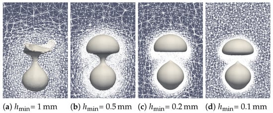
Figure 17.
Comparison of the experimental bubble profiles at time for different mesh sizes.
The impact of the mesh size was then quantitatively studied with respect to the variation of the following four key parameters of this study: vapor film thickness at mid height, vapor bubble volume, vapor bubble detachment frequency, and heat flux. The results are plotted in Figure 18.
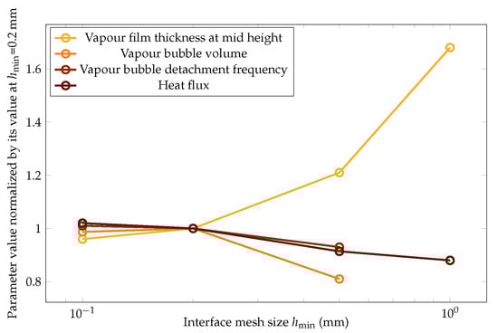
Figure 18.
The variation in the mean values of the vapor film thickness at mid height, vapor bubble volume, vapor bubble detachment frequency, and heat flux versus the mesh size. The values are normalized over the ones at , which was the parameter chosen for this study.
The four quantities converged to the same values at the finest mesh size within a 3% error. This error was considered acceptable to follow the study with the parameter .
6.3. Results and Comparison
6.3.1. First Application of the Model
A first batch of six simulations was conducted with these parameters without radiation (). Two qualitative comparisons with experimental results are presented in Figure 19 and Figure 20. Different pictures were considered over the period of formation of a vapor bubble . The associated sphere and bath temperatures were (, ) and (, ). We can see that the main features were respected for the configuration with high overheating and low subcooling. However, the production of vapor was greatly overestimated in the second configuration. This conclusion is supported by the comparison of the bubble shapes for all configurations (see Figure 21).

Figure 19.
Comparison of the experimental bubble profiles in the simulation for , .

Figure 20.
Comparison of the experimental bubble profiles in the simulation for , .

Figure 21.
Comparison of the simulated and experimental bubble profiles for different temperature configurations.
The simulation predictions for the vapor film mean thicknesses at the equator, bubble volume, detachment frequency, and surface heat fluxes were compared with the experimental results in Figure 22, Figure 23, Figure 24 and Figure 25. We could see that the mean thickness was overestimated by a factor of 1.5 in the configuration, as well as by a factor of 2 in the configuration. This was assumed to be due to the increased viscosity in the vapor film, which prevented the formation of thin vapor layers for a given vapor flow. The coarse mesh size in the liquid vapor could be a supplementary factor of error. However, the film thickness undergoes large variations in sizes that are one order of magnitude above the mesh size. Thus, this latter phenomenon might not be the dominant error factor. Regarding the bubble volumes, they were overestimated by the simulation, except in conditions of high overheating and low subcooling. This was assumed to be due to an underestimation of the liquid sides’ heat fluxes, which allow for larger vaporization. This argument also explains the overestimation of the vapor thickness. The detachment frequency of bubbles was more accurately measured. This confirms that the volume of the vapor is not the determining factor to describe the bubbles’ detachment. Moreover, it demonstrates that detachment remains unaffected by vapor viscosity, highlighting that it is, in fact, governed by the liquid flow. Finally, the heat fluxes were underestimated by a factor of two, which is consistent with the overestimation of the film thickness.
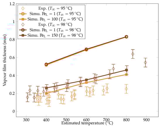
Figure 22.
Comparison of the experimental and simulated vapor film thicknesses at the equator of the sphere for liquid temperatures of and .
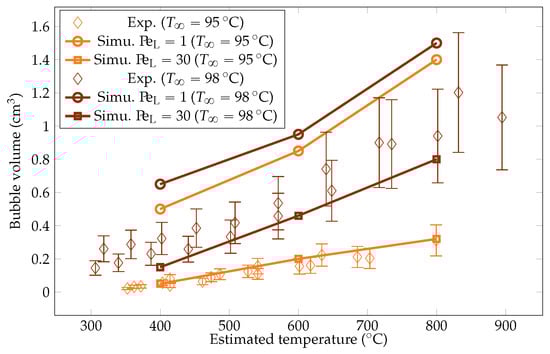
Figure 23.
Comparison of the experimental and simulated vapor bubble volumes for liquid temperatures of and .

Figure 24.
Comparison of the experimental and simulated vapor bubble detachment frequency for liquid temperatures of and .
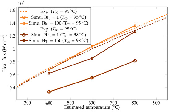
Figure 25.
Comparison of the experimental and simulated heat fluxes for the liquid temperatures of and .
6.3.2. Radiative Effects
To assess the influence of radiative effects, we considered the worst case scenario of a black body model (). We expected the influence of radiation to be dominant in the high overheating configuration, as the Stefan Bolzman law predicts heat fluxes that are only significant at this temperature range. To confirm this, the following two extreme configurations were simulated: , ; and , . The comparison criteria for the two emissivities are gathered in Table 4.
Table 4.
Comparison of the sphere-quenching simulations without radiation and with a black body model.
As expected, radiation effects are more significant during large overheating. The vapor production is increased, with larger vapor film and bigger bubbles. The heat flux is almost doubled. Lower overheating yields marginal parameter adjustments, though the heat flux is increased by 25%. It is worth noting that this assessment employs a conservative black body model, potentially overestimating radiative fluxes. In reality, radiative impact could be at least twice as small or even less, rendering radiation’s effect even more insignificant during low subcooling. We also noticed that the frequency remained unaltered, which once again confirms the independence of the vapor detachment on the vapor flow.
From these observations, we can conclude that the variations between the simulation and the experiment cannot be attributed to radiative effects. The deviation from experimental heat fluxes is still significant during high subcooling, and the vapor production is still overestimated.
6.3.3. Modification of the Liquid Conductivity at the Interface
An augmented vapor viscosity induces a more laminar regime in vapor film with straight velocity trajectories. This cancels the interfacial perturbations that are assumed to be the cause of an improved convection and, thus, improved heat fluxes on the liquid side close to the interface. These effects could account for the disparities between the simulation and the experiment, particularly at higher subcooling levels. In these cases, the simulations predict a greater vapor creation, which is not offset by condensation as expected.
To compensate for the elimination of this near-interface convection, a first model should evaluate it and deduce an equivalent thermal conductivity . The model of an equivalent thermal conductivity entails the assumption of a proportional relationship between the convective effects and subcooling. This thermal conductivity is then used when computing the heat flux jump at the interface.
A first estimation of convective heat fluxes reads as follows:
where is the normal velocity of the liquid close to the interface. This is equivalent to the replacement of a particle of temperature with a particle at a rate given by . If this phenomenon occurs on a thickness , then the equivalent thermal conductivity of this flux reads as follows:
We defined the associated Péclet number as the ratio of to :
In our experiment, the liquid’s normal velocity near the interface was observed to be . We estimated using the maximum amplitude of vapor film waves, which was approximately . This resulted in a value of around = −1 K−1 and .
To confirm this value, a sensitivity analysis on the heat flux was conducted by varying the at the highest overheating temperature () for both subcooling configurations. Results are plotted in Figure 26.

Figure 26.
Study of the influence of on the vapor heat flux for and .
We can see that an augmented improved a great deal of the heat fluxes. This is consistent as it reduced the vaporization and, thus, produced a thinner film. However, the value of (resp. ) seems to be the best approximation of the convective effects inside the liquid for (resp. ). This shows that is case-dependent, which would be consistent with the model of the liquid recirculation: the vapor film waves are indeed affected by the subcooling. However, the corresponding value was one order of magnitude higher than our former approximation, which was given by (35), meaning there will be a complex hydrodynamics at the liquid–vapor interface. Furthermore, these values of Péclet were at the lower bound as the simulations were run without radiation (0 emissivity). The addition of this effect would lead to an even stronger heat transfer from the liquid side to compensate for the additional heat on the energy balance at the interface.
To study the influence of the overheating on , we launched the six test cases for the two values of mentioned above. The resulting heat fluxes and interface thicknesses are plotted in Figure 22 and Figure 25. We observed that there was a lower bound on the interface thickness linked with the resolution of the mesh that the model could not overcome. However, the heat fluxes were still properly corrected, confirming that the information of the interface thickness at the equator is not sufficient to describe the system and that a complete modeling is necessary.
Snapshots of the interface for and are plotted in Figure 27 for different values of . Despite the convective model, the presence of undulation in the vapor film suggests that hydrodynamics within the vapor remained unaffected. Nonetheless, this model suppresses bubble formation. This phenomenon can be attributed to the reduced convective effects around the bubbles compared to the vapor film. Moreover, the liquid at the top of the sphere was heated up, which reduced the effect of the liquid convection. Consequently, also seemed to be spatially dependent.

Figure 27.
Comparison of the liquid–vapor interface behavior for different values of convective conductivities.
We aimed to determine the appropriate value that aligns with the convective effects during bubble ascent. We performed several simulations varying the values and compared the results with the experimental data, focusing on detached bubble behavior. The most promising outcome emerged with an order of magnitude around , corresponding to = 20 W m−1 K−1. Qualitative comparisons involving the interface behavior during vapor bubble formation were conducted for different test cases, as shown in Figure 28 and Figure 29. The associated sphere and bath temperatures were (, ) and (, ). This shows the capability of the solver to predict the bubble evolution, providing accurate computation of liquid-side heat fluxes. This is confirmed by the comparison of the bubble shapes across all the test cases (Figure 30) and volumes (Figure 23). Notably, the adjustments to influenced the bubble detachment frequency at low overheating conditions (Figure 24), which was attributed to the significant condensation on the upper surface of the bubble, thus impeding their growth.

Figure 28.
Comparison of the experimental bubble profiles with the simulation for and with the convective conductivity model for .

Figure 29.
Comparison of the experimental bubble profiles with the simulation for and with the convective conductivity model for .
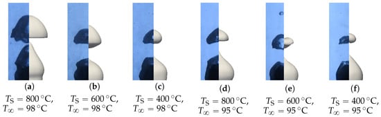
Figure 30.
Comparison of the simulated and experimental bubble profiles for different temperature configurations with the convective conductivity model for .
7. First Feedback on the Model
The current approach with augmented viscosity performs better for configurations with significant vaporization. This is consistent as characteristic lengths in the vapor phase are larger, leading to less viscosity-driven flows.
The model of convective conductivity in the liquid near the interface allows one to recover some of the features of the flow, but this is not universal. Moreover, no thermal steady state was reached in the simulation. This could change the values of . Further studies of this benchmark with finer meshes would be interesting. However, this still highlights the fundamental difference in intensity between the liquid convective effects within the liquid near the vapor film and those occurring over the vapor bubbles. A factor of five was found thanks to the comparison of the experimental and simulation results. To the best of the authors’ knowledge, such outcomes have not been previously reported in the literature. The authors believe that the configuration of film boiling allows for the presence of subtle Kelvin–Helmolz instabilities and results in small, but intense, convection cells on the liquid side. The study conducted by Honda et al. [22] showed that such instabilities facilitate convective motion that is significant enough to predict a good approximation of the vapor film thickness’ order of magnitude.
8. Conclusions and Perspectives
An experimental and numerical investigation of the film boiling mode around small spheres of nickel was tackled through this article. First, the focus of the experimental work was set on the vapor phase behavior using a thermocouple-free sphere to avoid, as much as possible, the interference with the support. Low subcoolings in the vicinity of were chosen to guarantee the production of a large amount of vapor. The results show that the influence of subcooling was mainly linked with hydrodynamics, whereas the heat fluxes were less affected. This means that the subcooling impacted the distribution on the energy evacuated between the creation of vapor and the warming of the liquid more, but less than the absolute value of the total energy evacuated. It also significantly influenced the Leidenfrost temperature value, confirming the findings in the literature. These conclusions remain limited in the vicinity of ; thus, a numerical simulation of such a system was proposed. The computation relies on a finite element library, with a Level Set approach to model the interface. Due to numerical challenges, a simplified view of the flow was simulated thanks to the consideration of an augmented viscosity. The comparison of the numerical simulation with experimental results led to the conclusion that the convective effects within the liquid near the vapor film were pronounced. However, these effects were limited to the film adjacent to the sphere, with less intense convective effects over the sphere itself (factor of five). This latter conclusion shall be taken qualitatively with respect to the remaining difference in prediction between the experimental and numerical results.
Enhanced temperature and heat flux estimations could be achieved through experiments with reduced uncertainties. An improvement could involve extending the camera set up to capture the entire vapor film, allowing for a better correlation estimation between the vapor film thickness and heat fluxes. Additionally, broader ranges of subcooling could be explored. In terms of simulation, improving the stability of the model would enhance the ability to predict the physical phenomenon accurately.
Author Contributions
Conceptualization, C.B., L.C.-B., R.C. and R.V.; methodology, C.B., L.C.-B., R.C. and R.V.; software, C.B. and E.H.; validation, C.B., L.C.-B., R.C. and R.V.; formal analysis, C.B., L.C.-B., R.C. and R.V.; investigation, C.B., L.C.-B., R.C. and R.V.; resources, R.C. and R.V.; data curation, C.B. and L.C.-B.; writing—original draft preparation, C.B.; writing—review and editing, C.B., L.C.-B., R.C. and R.V.; visualization, C.B., L.C.-B. and R.C.; supervision, R.C., E.H. and R.V.; project administration, E.H. and R.V.; funding acquisition, E.H. All authors have read and agreed to the published version of the manuscript.
Funding
This research was funded by French National Research Agency (ANR) under grant number [ANR-17-CHIN-0003].
Data Availability Statement
No additional data are available for this work.
Acknowledgments
The authors gratefully acknowledge support from the companies involved in the INFINITY industrial chair: Aubert & Duval, Cevifal, CMI Group, Faurecia, Framatome, Industeel CRMC (Arcelor Mittal), Lisi Aerospace, Montupet, Safran, Science Computer and Consultants (SCC), and Transvalor.
Conflicts of Interest
The authors declare that they have no conflicts of interest.
Nomenclature
| Variables | |
| t | Time () |
| Velocity vector (m s−1) | |
| P | Pressure () |
| T | Temperature () |
| Cooling rate (K s−1) | |
| Heat flux vector (W m−2) | |
| Strain rate tensor (s−1) | |
| Surface mass transfer rate vector (kg s−1 m−2) | |
| Surface tension vector (J m−2) | |
| e | Mean vapor film thickness () |
| Vapor bubble volume at detachment () | |
| f | Vapor bubble detachment frequency (K1/4 s−1) |
| Parameters | |
| Temperature gap with saturation temperature () | |
| Density (kg m−3) | |
| Specific heat capacity at constant pressure (J K−1 kg−1) | |
| k | Thermal conductivity (W K−1 m−1) |
| D | Thermal diffusivity (m−2 s−1) |
| Emissivity (-) | |
| Dynamic viscosity () | |
| Surface tension coefficient (J m−2) | |
| Specific enthalpy of vaporization at saturation temperature (J kg−1) | |
| Gravity vector (m s−1) | |
| A | Proportionality coefficient of the heat flux model () |
| Time step () | |
| h | Mesh size () |
| Subscripts | |
| Liquid | |
| Vapor | |
| Sphere | |
| Saturation temperature of the fluid at atmospheric pressure | |
| ∞ | Subcooling |
| R | Radiation |
| Minimum heat flux | |
| i | Initial state of the sphere before the quench |
| Experimental value | |
| Vapor creation rate | |
| Minimum mesh size | |
| Mathematical and | |
| geometrical functions | |
| Normal vector of the liquid–vapor interface (-) | |
| Level Set function () | |
| Heaviside function (-) | |
| Dirac function () | |
| Curvature () | |
| Characteristic length of the smoothed interface () | |
| Gradient operator | |
| Divergence operator |
References
- Nukiyama, S. The maximum and minimum values of the heat Q from metal to boilng water under atmospheir pressure. J. Jpn. Soc. Mech. Eng. 1934, 37, 367–374. [Google Scholar]
- Zuber, N. Hydrodynamic Aspects of Boiling Heat Transfer. Technical Report. Ph.D. Thesis, University of California, Berkeley, CA, USA, 1959. [Google Scholar] [CrossRef]
- Berenson, P.J. Transition Boiling Heat Transfer from a Horizontal Surface; Technical Report 17; The National Science Foundation, Massachusetts Institude of Technology: Cambridge, MA, USA, 1960. [Google Scholar]
- Chen, J.C. Correlation for Boiling Heat Transfer to Saturated Fluids in Convective Flow. Ind. Eng. Chem. Process Des. Dev. 1966, 5, 322–329. [Google Scholar] [CrossRef]
- Judd, R.L.; Hwang, K.S. A Comprehensive Model for Nucleate Pool Boiling Heat Transfer Including Microlayer Evaporation. J. Heat Transf. 1976, 98, 623–629. [Google Scholar] [CrossRef]
- Cooper, M. Saturation Nucleate Pool Boiling—A Simple Correlation; Elsevier: Amsterdam, The Netherlands, 1984; pp. 785–793. [Google Scholar] [CrossRef]
- Ramilison, J.M.; Lienhard, J.H. Transition Boiling Heat Transfer and the Film Transition Regime. J. Heat Transf. 1987, 109, 746–752. [Google Scholar] [CrossRef]
- Steiner, H.; Kobor, A.; Gebhard, L. A wall heat transfer model for subcooled boiling flow. Int. J. Heat Mass Transf. 2005, 48, 4161–4173. [Google Scholar] [CrossRef]
- Meduri, P.K.; Warrier, G.R.; Dhir, V.K. Wall heat flux partitioning during subcooled forced flow film boiling of water on a vertical surface. Int. J. Heat Mass Transf. 2009, 52, 3534–3546. [Google Scholar] [CrossRef]
- Brennen, C.E. Fundamentals of Multiphase Flow, Reprint ed.; Cambridge Univ. Press: Cambridge, UK, 2006; OCLC: 316280080. [Google Scholar]
- Samuel, A.; Prabhu, K.N. Residual Stress and Distortion during Quench Hardening of Steels: A Review. J. Mater. Eng. Perform. 2022, 31, 5161–5188. [Google Scholar] [CrossRef]
- Canale, L.d.C.F.; Totten, G.E. Quenching technology: A selected overview of the current state-of-the-art. Mater. Res. 2005, 8, 461–467. [Google Scholar] [CrossRef]
- Vijaykumar, R.; Dhir, V.K. An Experimental Study of Subcooled Film Boiling on a Vertical Surface—Thermal Aspects. J. Heat Transf. 1992, 114, 169–178. [Google Scholar] [CrossRef]
- Klimenko, V. Film boiling on a horizontal plate—New correlation. Int. J. Heat Mass Transf. 1981, 24, 69–79. [Google Scholar] [CrossRef]
- Kolev, N. Film boiling on vertical plates and spheres. Exp. Therm. Fluid Sci. 1998, 18, 97–115. [Google Scholar] [CrossRef]
- Kaneyasu, N.; Takehiro, I. Two-phase boundary-layer treatment of free-convection film boiling. Int. J. Heat Mass Transf. 1966, 9, 103–115. [Google Scholar] [CrossRef]
- Vijaykumar, R.; Dhir, V.K. An Experimental Study of Subcooled Film Boiling on a Vertical Surface—Hydrodynamic Aspects. J. Heat Transf. 1992, 114, 161–168. [Google Scholar] [CrossRef]
- Dhir, V.; Purohit, G. Subcooled film-boiling heat transfer from spheres. Nucl. Eng. Des. 1978, 47, 49–66. [Google Scholar] [CrossRef]
- Jouhara, H.; Axcell, B.P. Film boiling heat transfer and vapour film collapse on spheres, cylinders and plane surfaces. Nucl. Eng. Des. 2009, 239, 1885–1900. [Google Scholar] [CrossRef]
- Das, D.C.; Ghosh, K.; Sanyal, D. A scale analysis model for film boiling heat transfer on a vertical flat plate with wide applicability. Int. J. Heat Mass Transf. 2015, 90, 40–48. [Google Scholar] [CrossRef]
- Baudin, N. Etude Expérimentale et Modélisation de L’ébullition Transitoire. Ph.D. Thesis, Université de Toulouse, Toulouse, France, 2015. [Google Scholar]
- Honda, H.; Makishi, O.; Yamashiro, H. Generalized stability theory of vapor film in subcooled film boiling on a sphere. Int. J. Heat Mass Transf. 2007, 50, 3390–3400. [Google Scholar] [CrossRef]
- Ebrahim, S.A.; Chang, S.; Cheung, F.B.; Bajorek, S.M. Parametric investigation of film boiling heat transfer on the quenching of vertical rods in water pool. Appl. Therm. Eng. 2018, 140, 139–146. [Google Scholar] [CrossRef]
- Feng, Q.; Johannsen, K. Experimental results of maximum transition boiling temperature during upflow in a circular tube at medium pressure. Exp. Therm. Fluid Sci. 1991, 4, 90–102. [Google Scholar] [CrossRef]
- Ikkene, R.; Koudil, Z.; Mouzali, M. Pouvoir de refroidissement des solutions de trempe à base de polymères hydrosolubles. CR Chim. 2008, 11, 297–306. [Google Scholar] [CrossRef]
- Burns, R.A. Heat Transfer Studies with Application to Nuclear Reactors. Ph.D. Thesis, The University of Manchester (United Kingdom), Manchester, UK, 1989. [Google Scholar]
- Whitaker, S. Forced convection heat transfer correlations for flow in pipes, past flat plates, single cylinders, single spheres, and for flow in packed beds and tube bundles. Aiche J. 1972, 18, 361–371. [Google Scholar] [CrossRef]
- Greene, G.A.; Irvine, T.F. The Effect of Water Subcooling on Film Boiling Heat Transfer from Vertical Cylinders; Office of Scientific and Technical Information, 1994; pp. 940809–940815. Available online: https://www.osti.gov/biblio/10135337 (accessed on 19 May 2025).
- Howard, A.H.; Mudawar, I. Orientation effects on pool boiling critical heat flux (CHF) and modeling of CHF for near-vertical surfaces. Int. J. Heat Mass Transf. 1999, 42, 1665–1688. [Google Scholar] [CrossRef]
- Tripathi, M.K.; Sahu, K.C.; Govindarajan, R. Dynamics of an initially spherical bubble rising in quiescent liquid. Nat. Commun. 2015, 6, 6268. [Google Scholar] [CrossRef]
- Hosler, E.R.; Westwater, J.W. Film Boiling on a Horizontal Plate. Ars J. 1962, 32, 553–558. [Google Scholar] [CrossRef]
- Sato, Y.; Ničeno, B. A sharp-interface phase change model for a mass-conservative interface tracking method. J. Comput. Phys. 2013, 249, 127–161. [Google Scholar] [CrossRef]
- Gibou, F.; Chen, L.; Nguyen, D.; Banerjee, S. A level set based sharp interface method for the multiphase incompressible Navier–Stokes equations with phase change. J. Comput. Phys. 2007, 222, 536–555. [Google Scholar] [CrossRef]
- Tanguy, S.; Sagan, M.; Lalanne, B.; Couderc, F.; Colin, C. Benchmarks and numerical methods for the simulation of boiling flows. J. Comput. Phys. 2014, 264, 1–22. [Google Scholar] [CrossRef]
- Sahut, G.; Ghigliotti, G.; Balarac, G.; Bernard, M.; Moureau, V.; Marty, P. Numerical simulation of boiling on unstructured grids. J. Comput. Phys. 2021, 432, 110161. [Google Scholar] [CrossRef]
- Giustini, G.; Issa, R.I. A method for simulating interfacial mass transfer on arbitrary meshes. Phys. Fluids 2021, 33, 087102. [Google Scholar] [CrossRef]
- Brissot, C.; Cailly-Brandstäter, L.; Hachem, E.; Valette, R. A Vaporization Model for Continuous Surface Force Approaches and Subcooled Configurations. Fluids 2023, 8, 233. [Google Scholar] [CrossRef]
- Patankar, S.V. Numerical Heat Transfer and Fluid Flow; Series in Computational Methods in Mechanics and Thermal Sciences; Hemisphere Publ. Co.: New York, NY, USA, 1980; OCLC: 31743097. [Google Scholar]
- Hachem, E.; Kloczko, T.; Digonnet, H.; Coupez, T. Stabilized finite element solution to handle complex heat and fluid flows in industrial furnaces using the immersed volume method. Int. J. Numer. Meth. Fluids 2010, 68, 99–121. [Google Scholar] [CrossRef]
- Unverdi, S.O.; Tryggvason, G. A Front-Tracking Method for Viscous, Incompressible, Multi-fluid Flows. J. Comput. Phys. 1992, 100, 25–37. [Google Scholar] [CrossRef]
- Sussman, M.; Smereka, P.; Osher, S. A Level Set Approach for Computing Solutions to Incompressible Two-Phase Flows. J. Comput. Phys. 1994, 114, 146–159. [Google Scholar] [CrossRef]
- Osher, S.; Fedkiw, R. Level Set Methods and Dynamic Implicit Surfaces; Applied Mathematical Sciences; Springer: Berlin/Heidelberg, Germany, 2004; Volume 153. [Google Scholar]
- Khalloufi, M.; Mesri, Y.; Valette, R.; Massoni, E.; Hachem, E. High fidelity anisotropic adaptive variational multiscale method for multiphase flows with surface tension. Comput. Method Appl. M 2016, 307, 44–67. [Google Scholar] [CrossRef]
- Brackbill, J.; Kothe, D.; Zemach, C. A continuum method for modeling surface tension. J. Comput. Phys. 1992, 100, 335–354. [Google Scholar] [CrossRef]
- Hysing, S. A new implicit surface tension implementation for interfacial flows. Int. J. Numer. Methods Fluids 2006, 51, 659–672. [Google Scholar] [CrossRef]
- Raessi, M.; Bussmann, M.; Mostaghimi, J. A semi-implicit finite volume implementation of the CSF method for treating surface tension in interfacial flows. Int. J. Numer. Methods Fluids 2009, 59, 1093–1110. [Google Scholar] [CrossRef]
- Denner, F.; van Wachem, B.G. Numerical time-step restrictions as a result of capillary waves. J. Comput. Phys. 2015, 285, 24–40. [Google Scholar] [CrossRef]
- Khalloufi, M. Multiphase Flows with Phase Change and Boiling in Quenching Processes. Ph.D. Thesis, Mines ParisTech, Paris, France, 2018. [Google Scholar]
- Haynes, W.M. CRC Handbook of Chemistry and Physics; CRC Press: Boca Raton, FL, USA, 2016; p. 2643. [Google Scholar]
- Movaghar, A.; Chiodi, R.; Desjardins, O.; Oevermann, M.; Kerstein, A.R. A Subgrid-Scale Model for Large-Eddy Simulation of Liquid/Gas Interfaces Based on One-Dimensional Turbulence. In Turbulent Cascades II; Springer: Berlin/Heidelberg, Germany, 2019; pp. 83–91. [Google Scholar]
- Chiodi, R.; McCaslin, J.; Desjardins, O. Interactions Between Turbulence and Interfaces with Surface Tension. In Turbulent Cascades II; Springer: Berlin/Heidelberg, Germany, 2019; pp. 249–256. [Google Scholar]
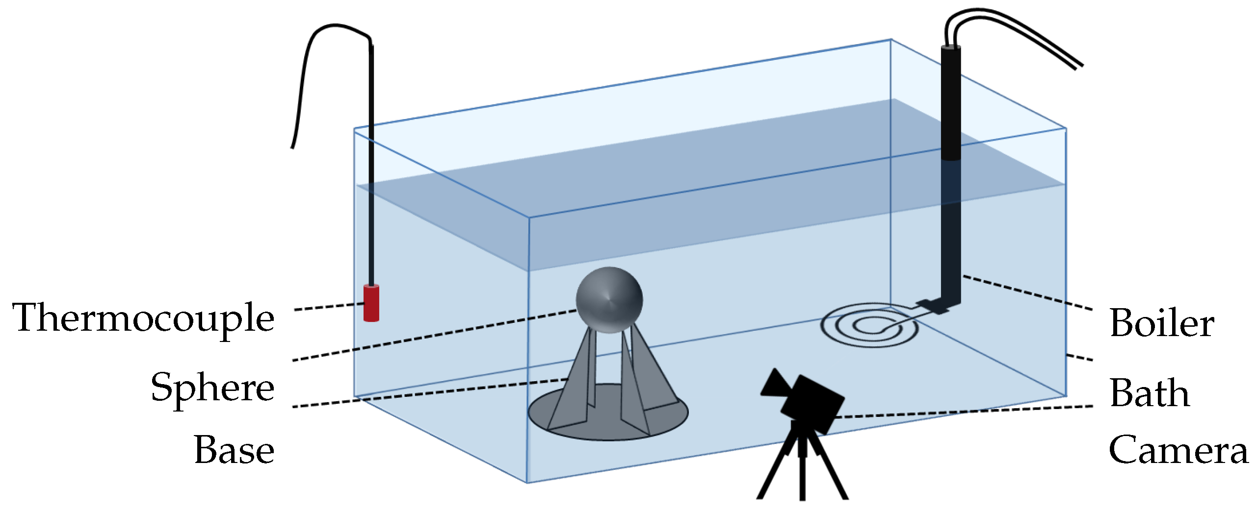
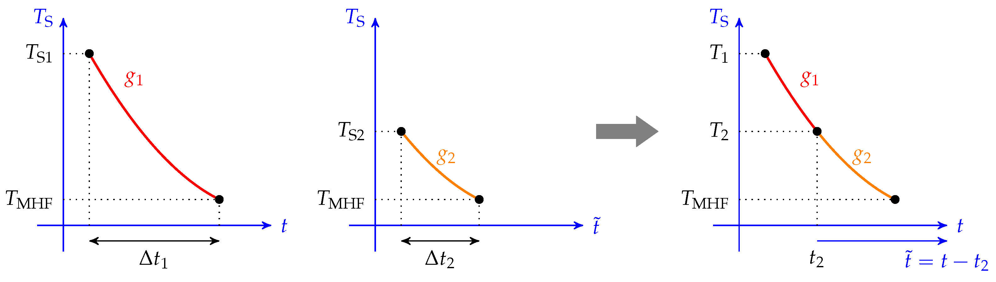
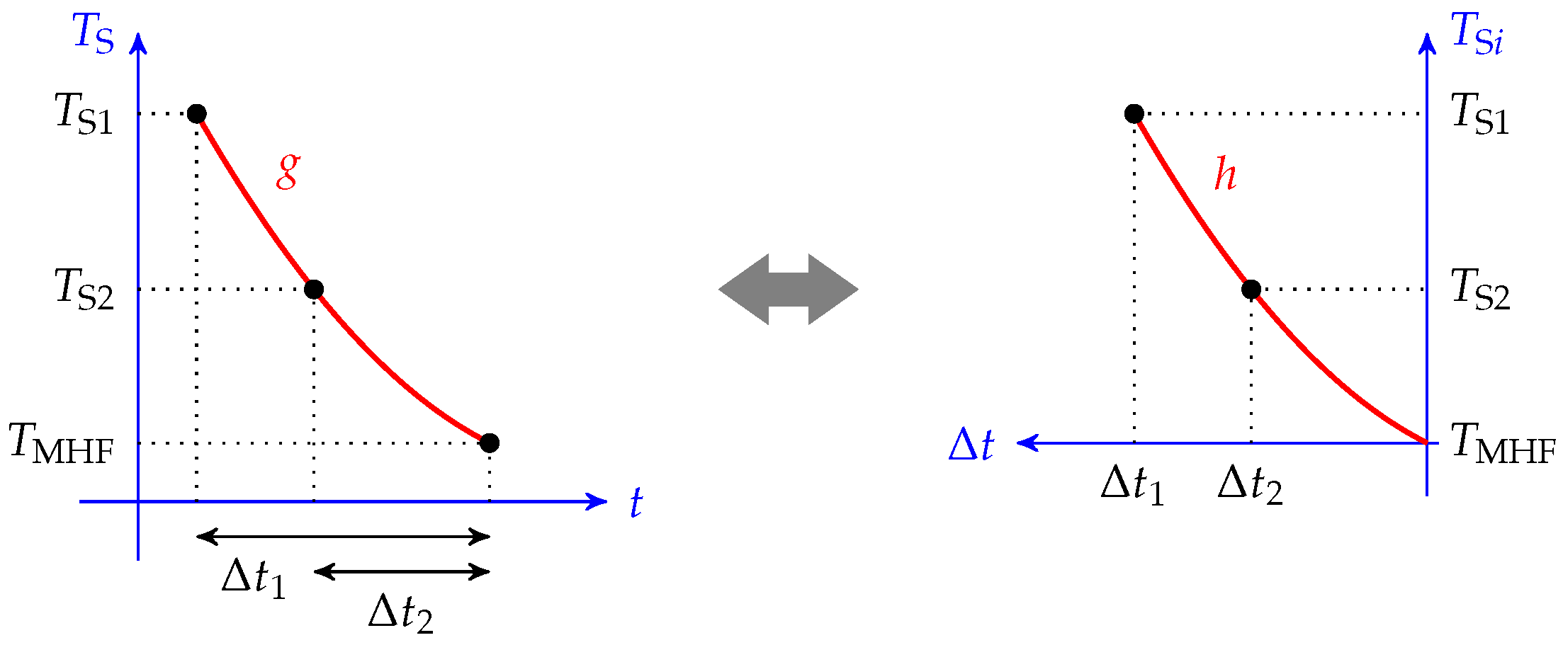
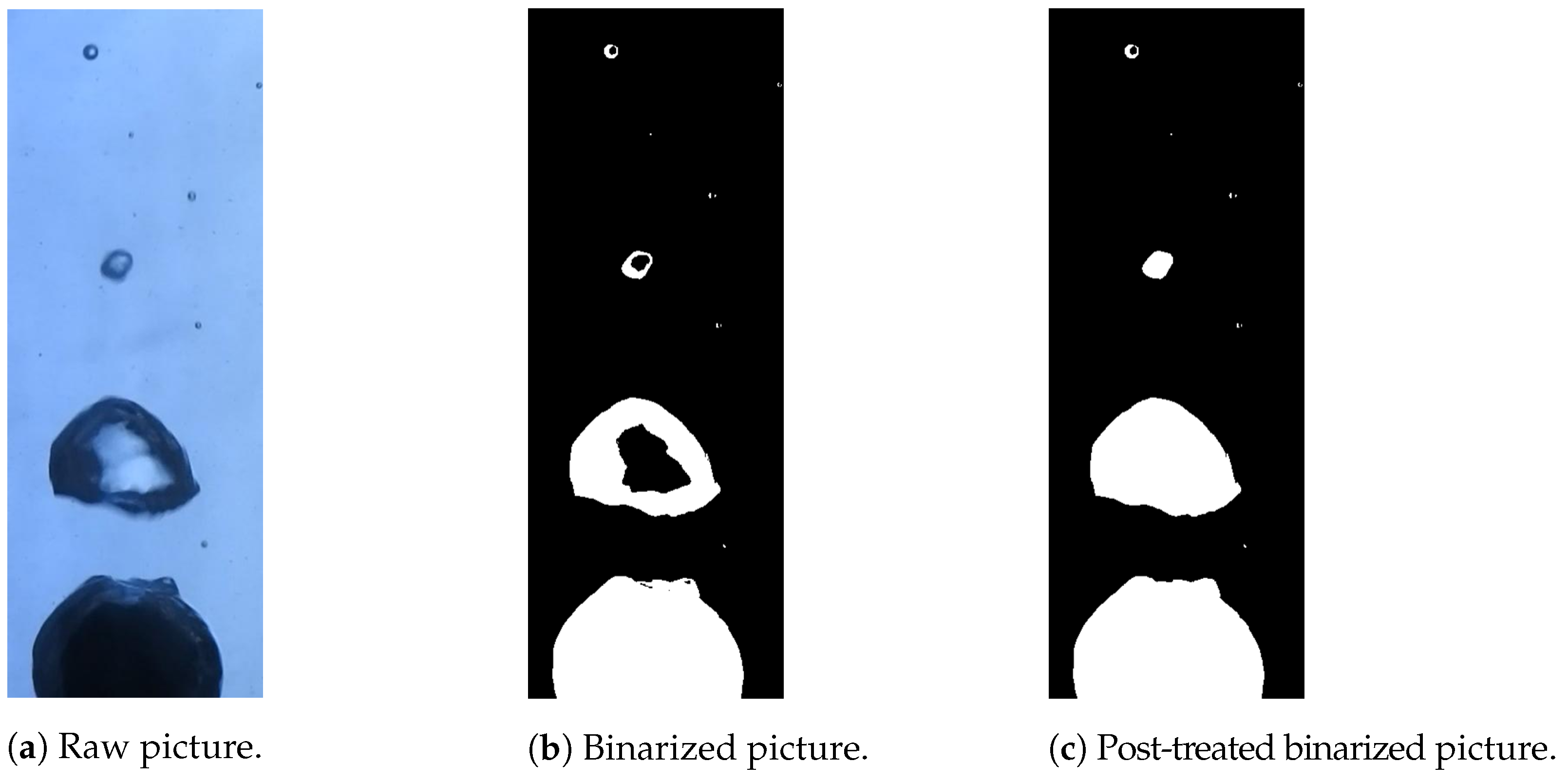
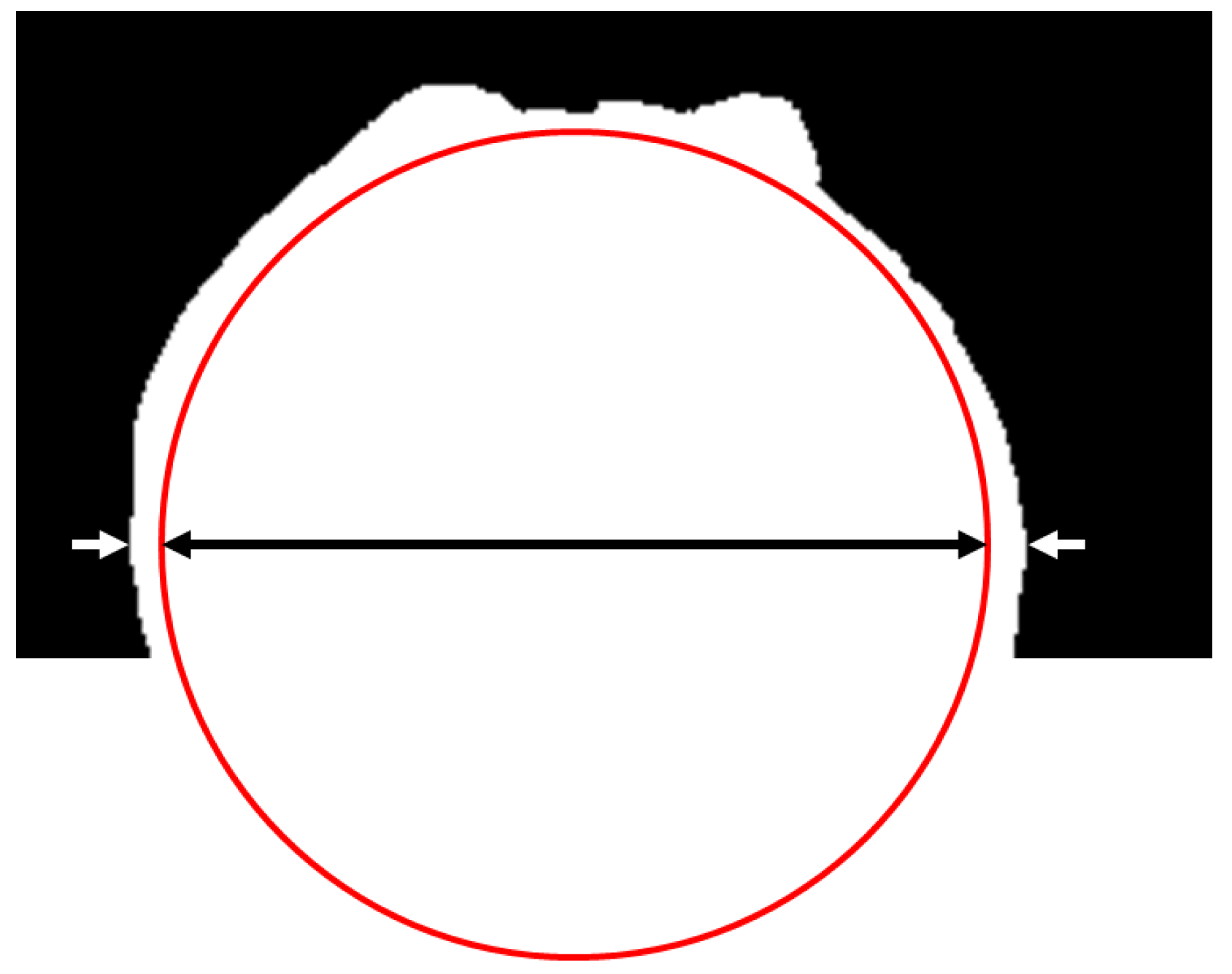
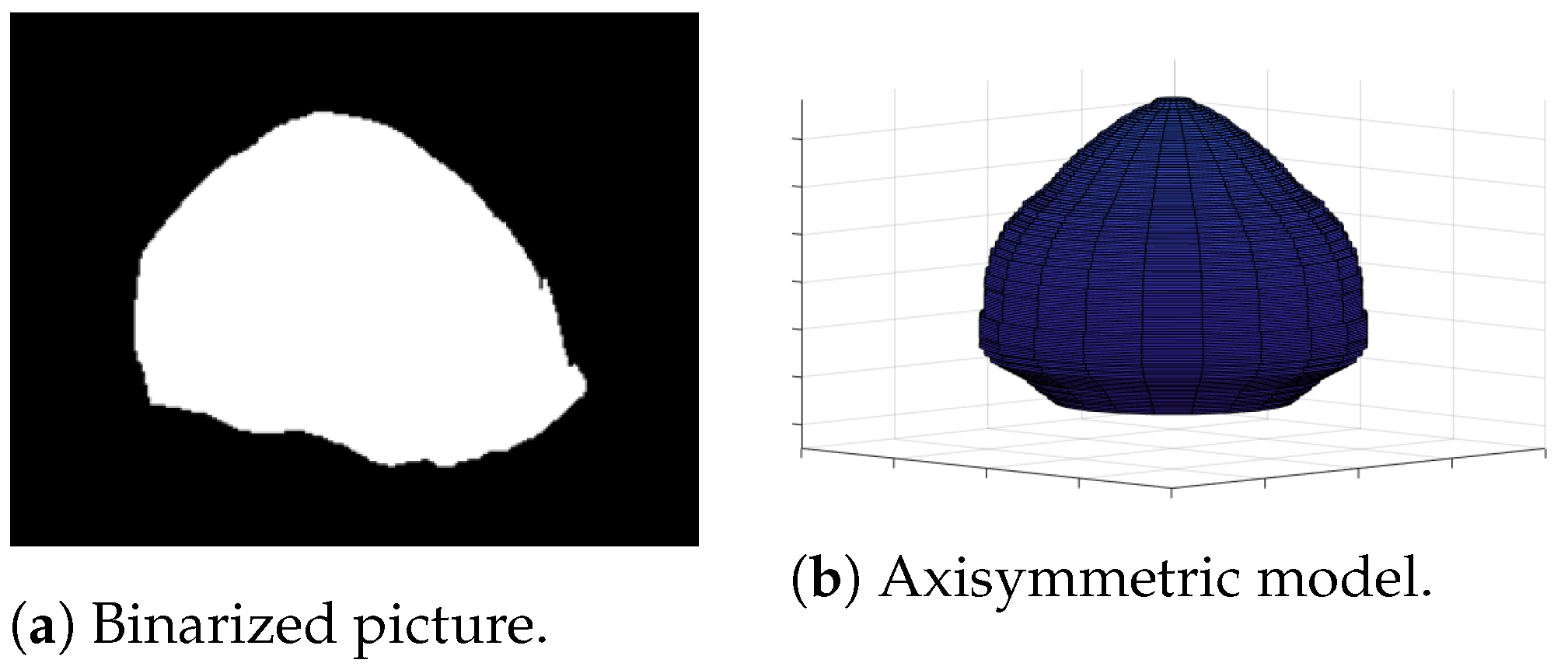
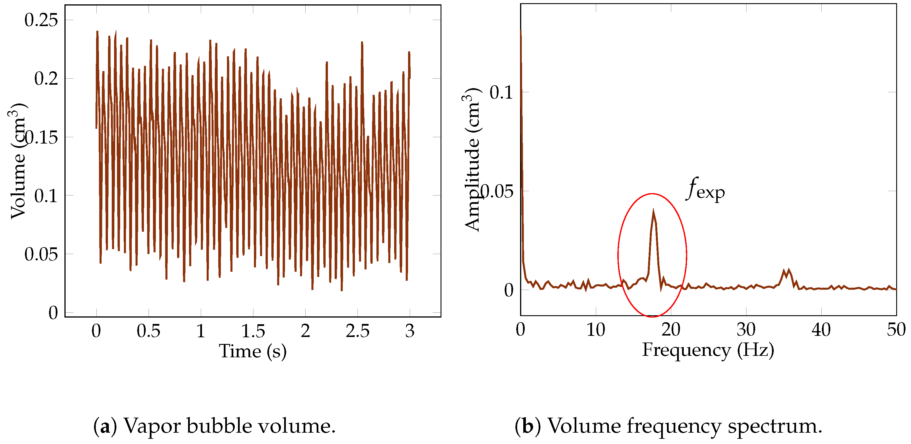
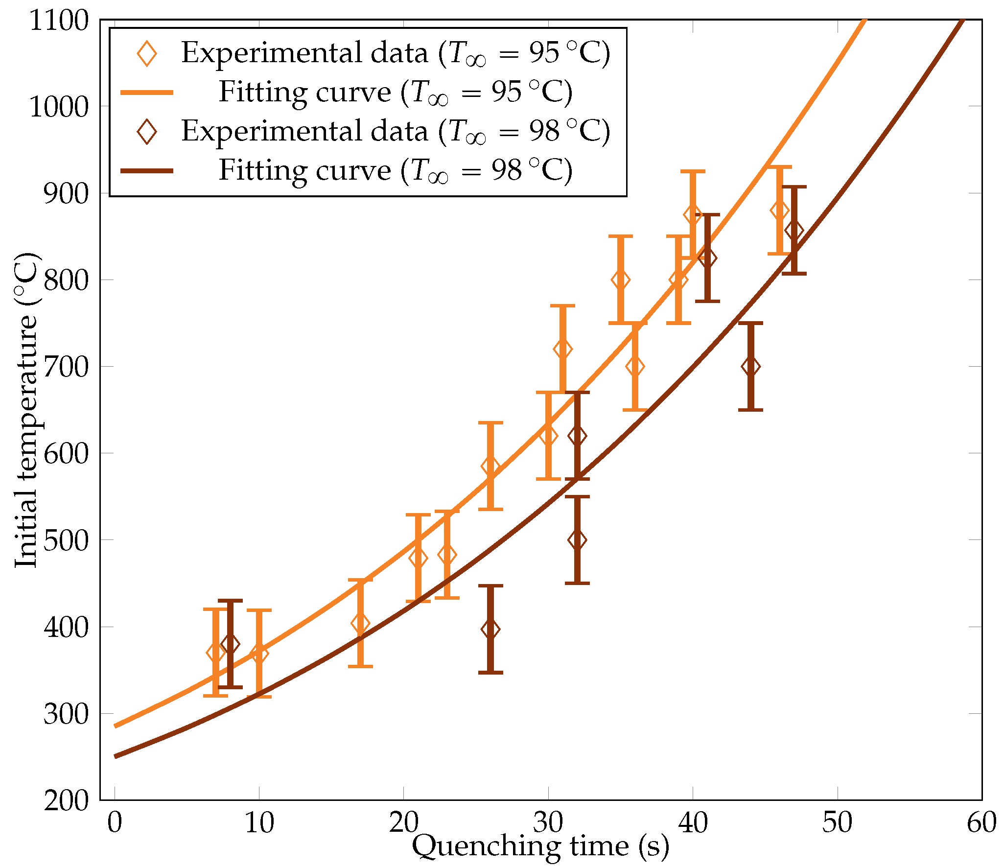
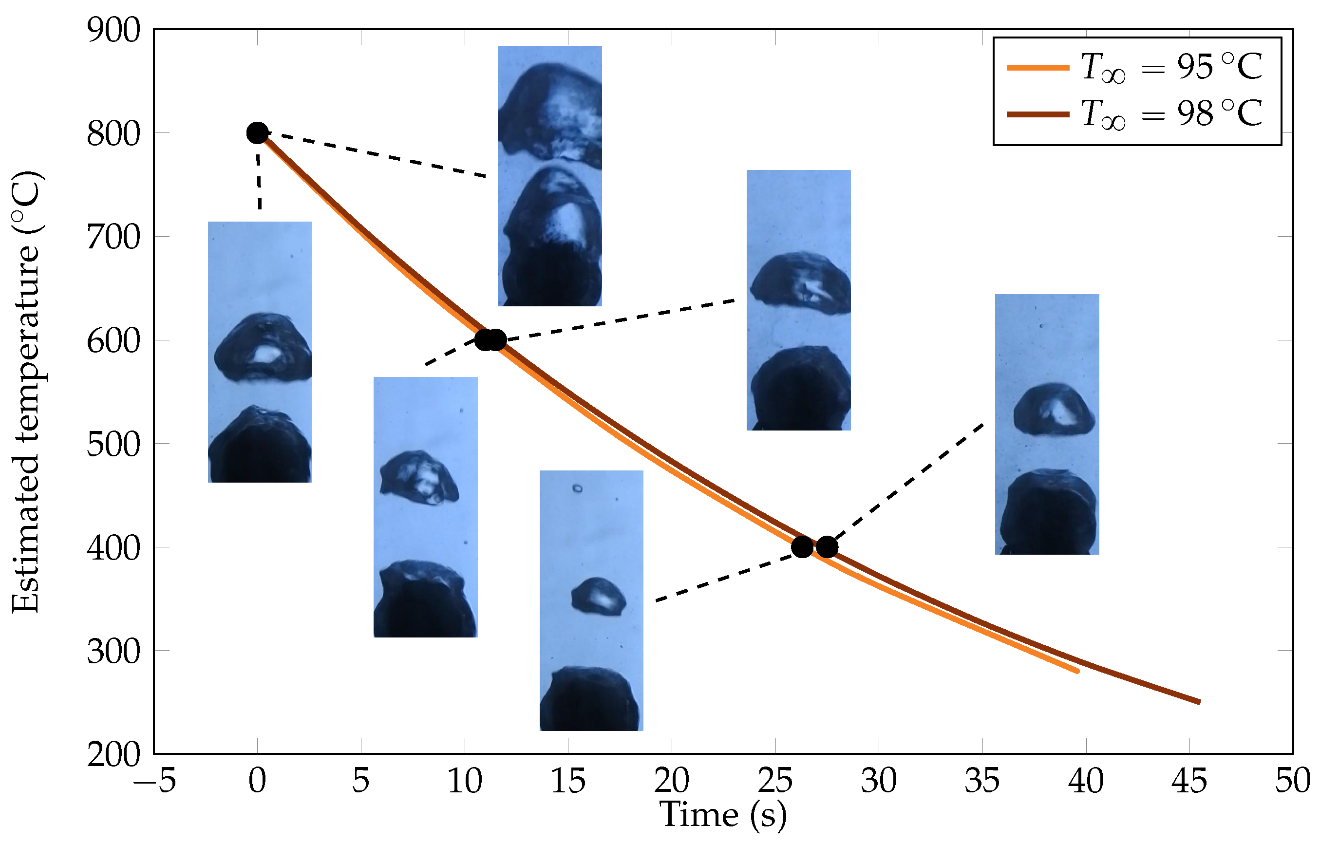
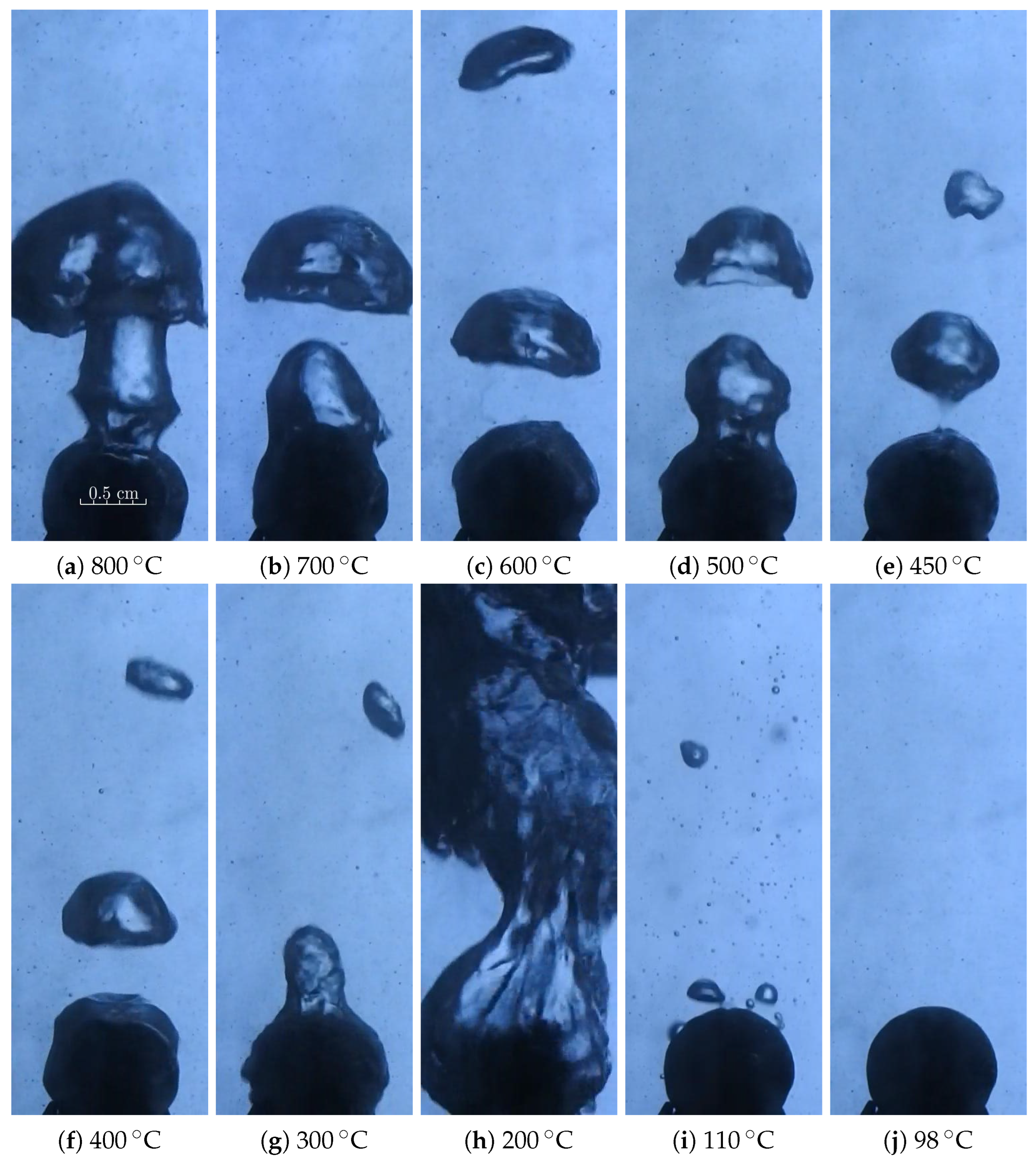
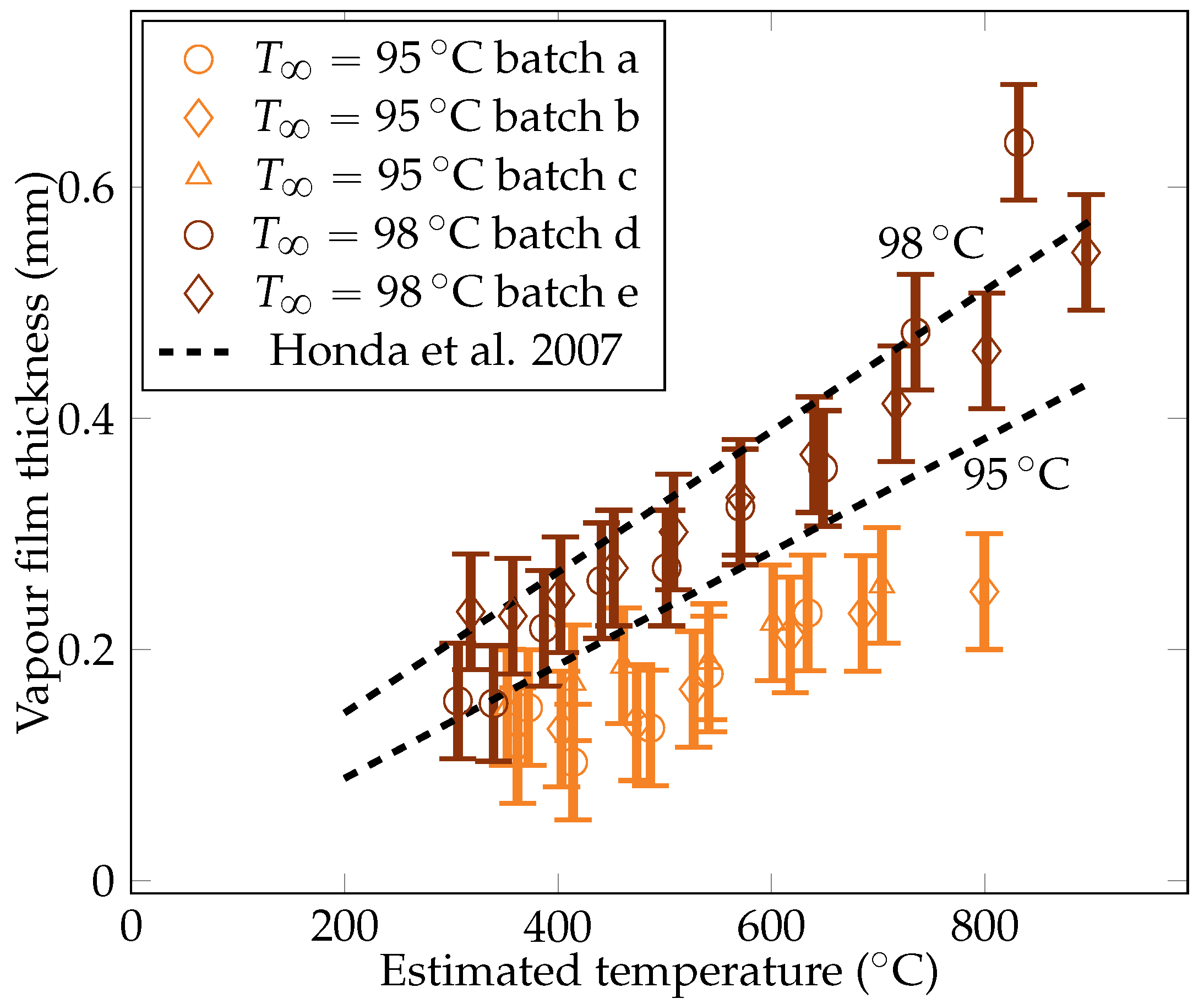
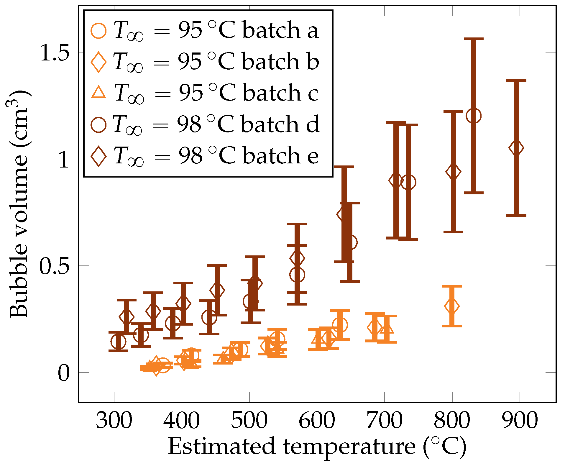
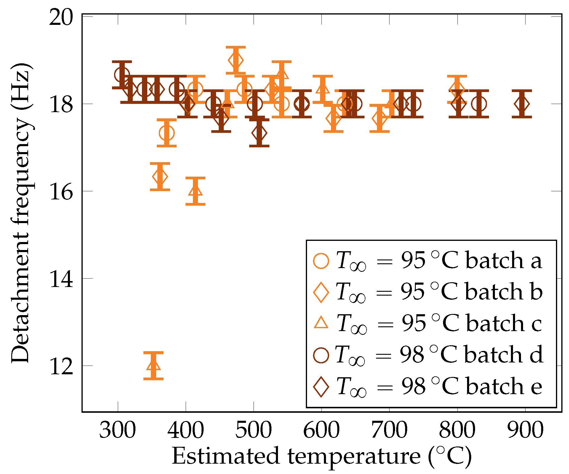
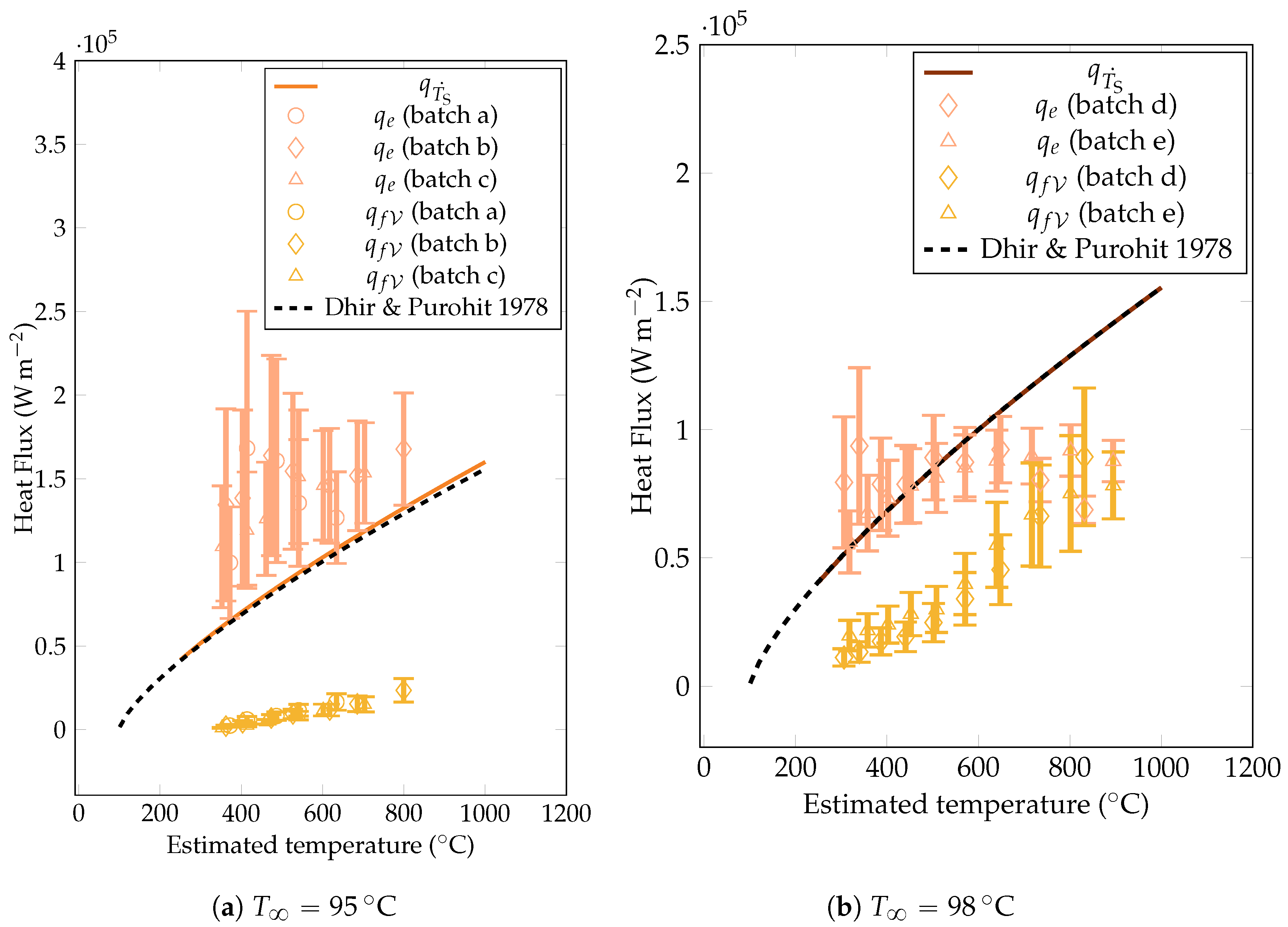
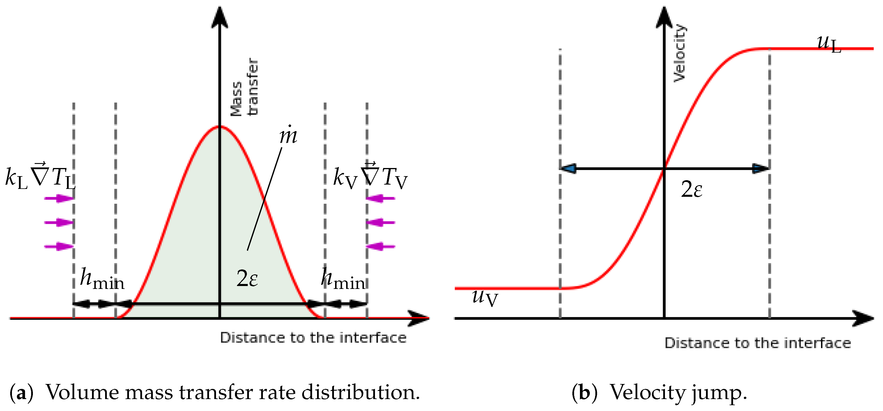
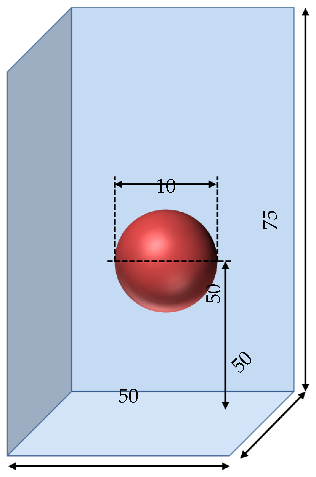
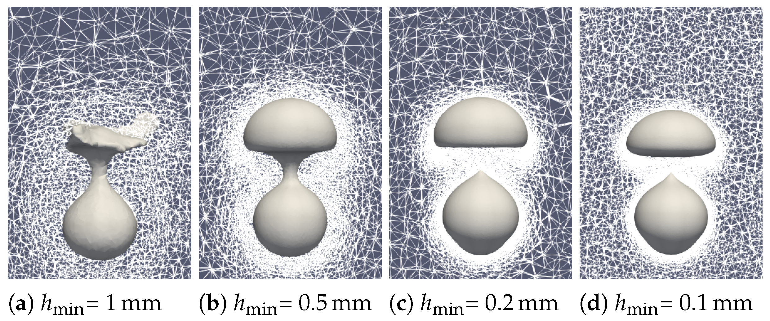
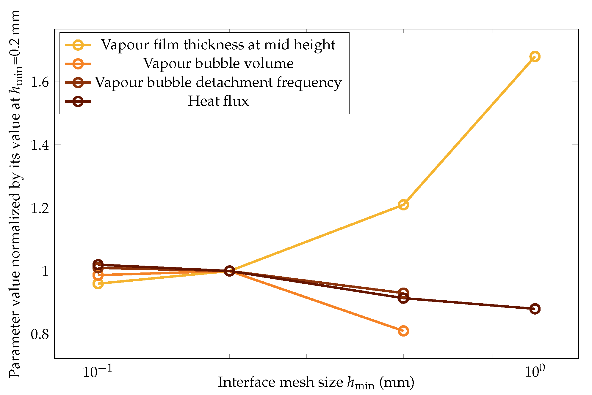
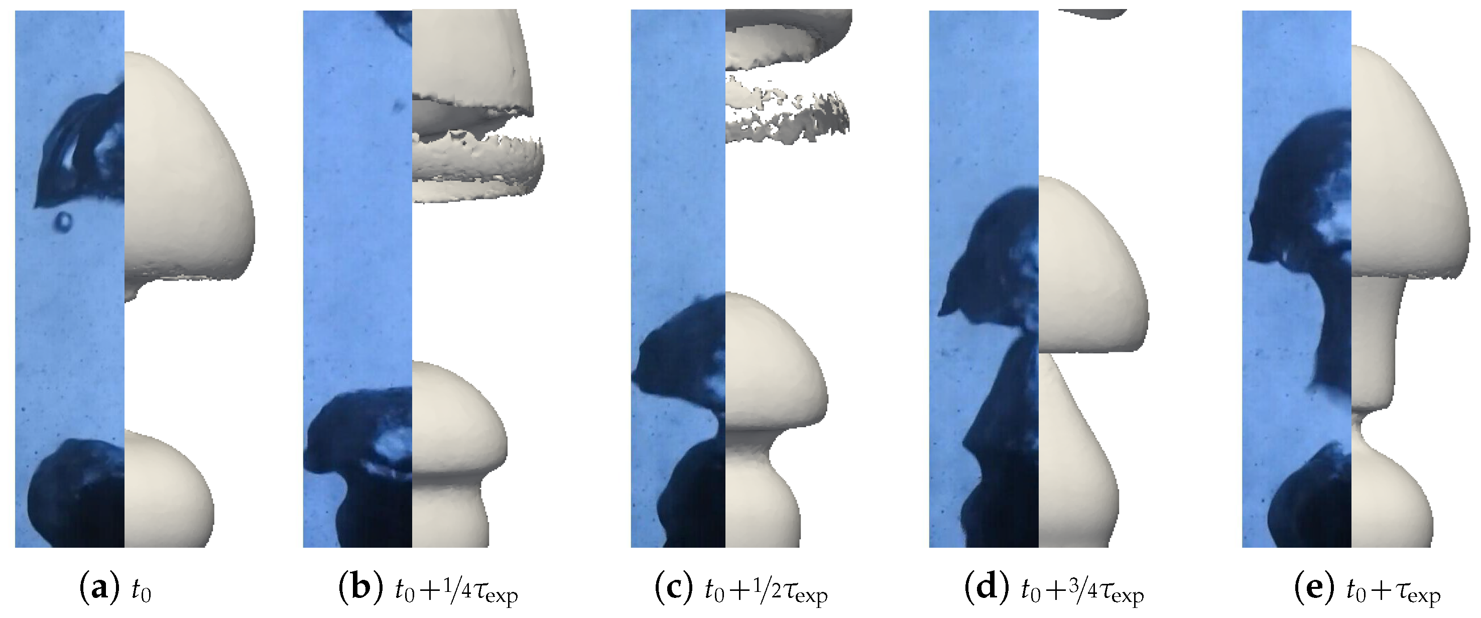
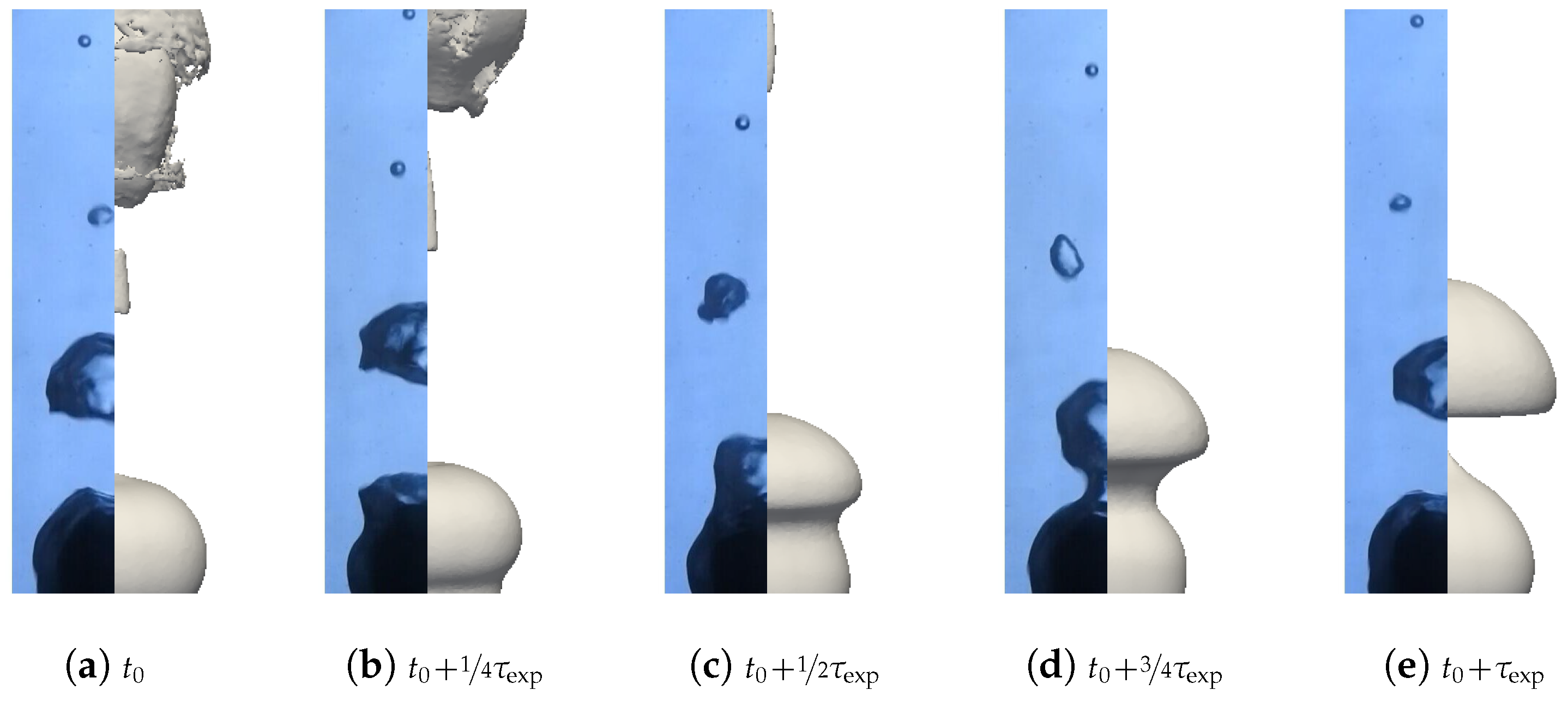
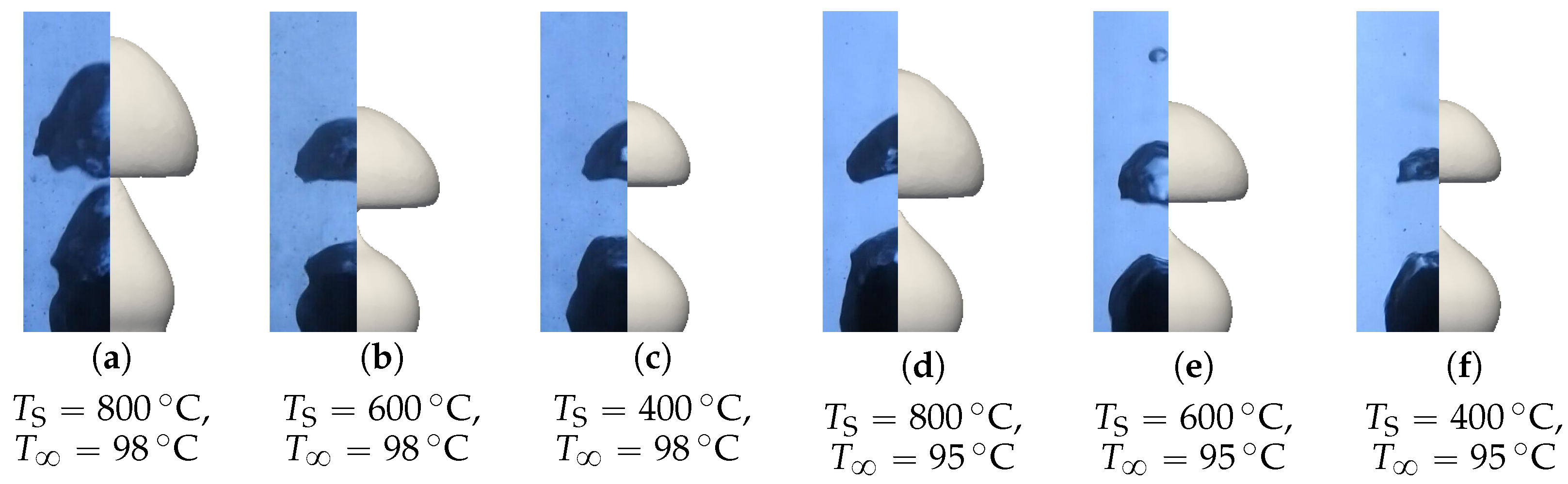
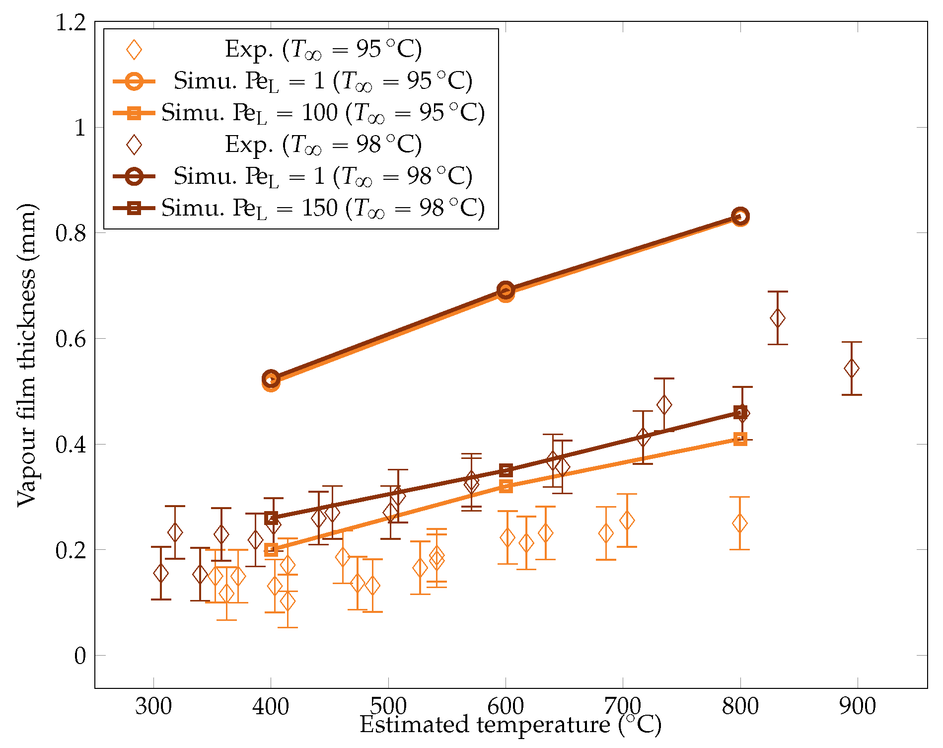
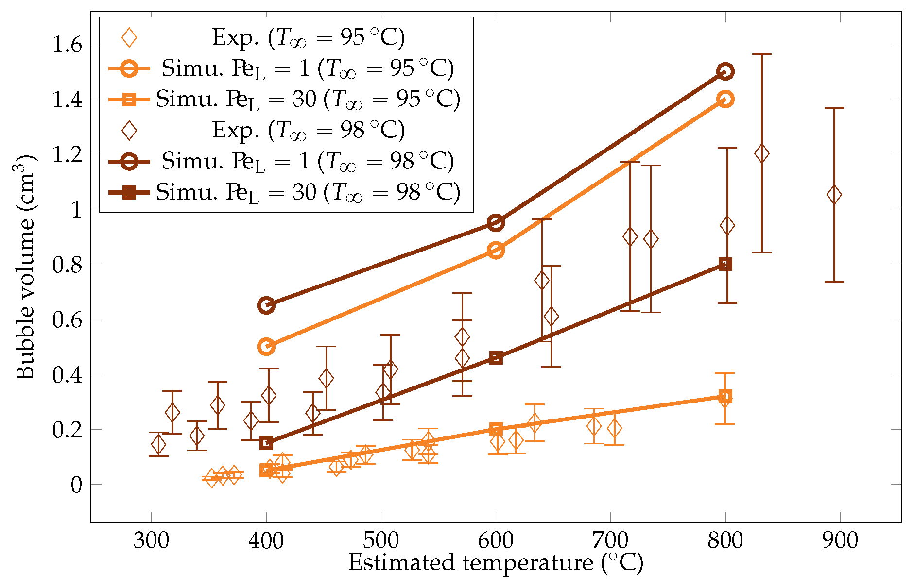
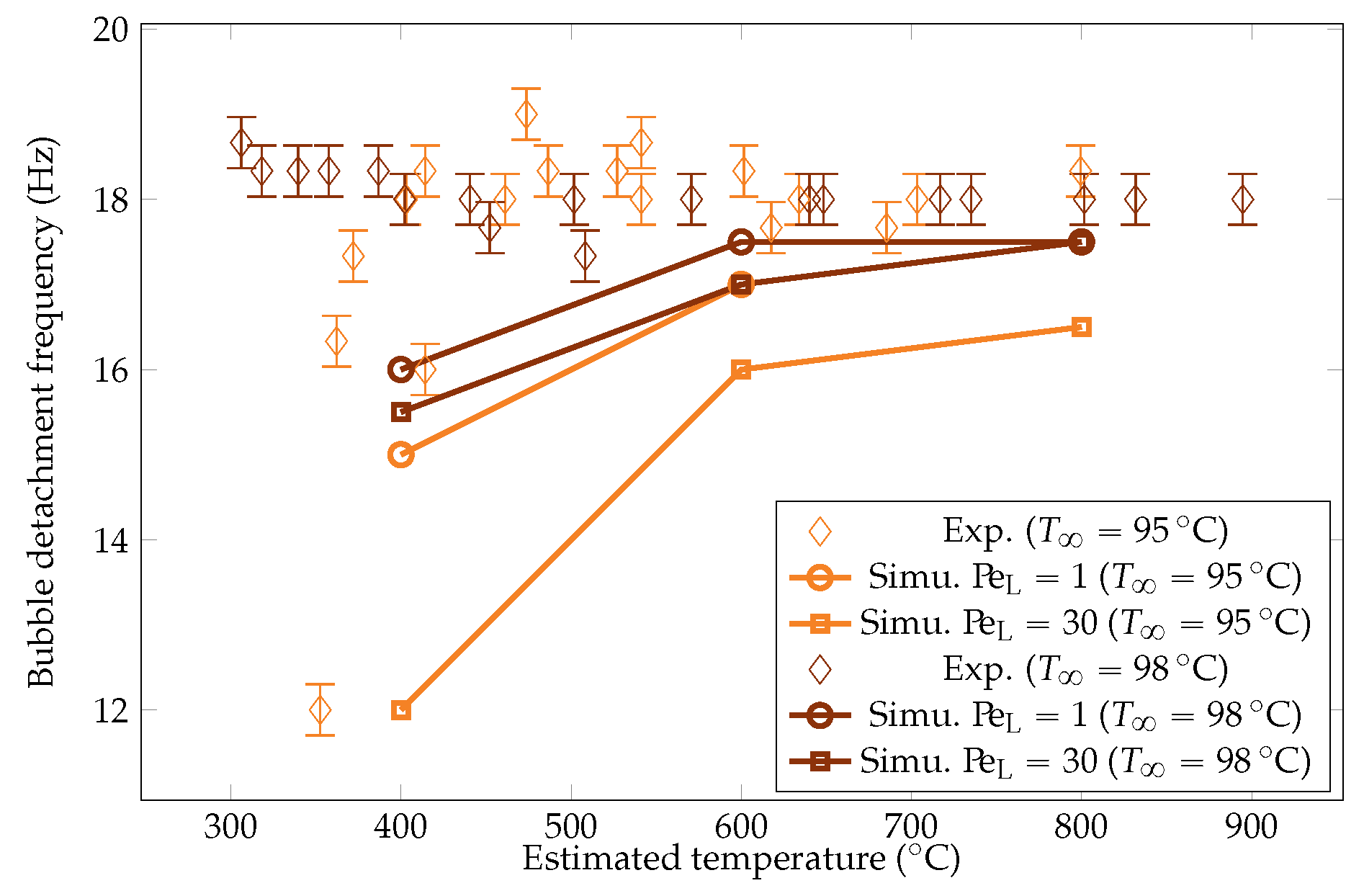

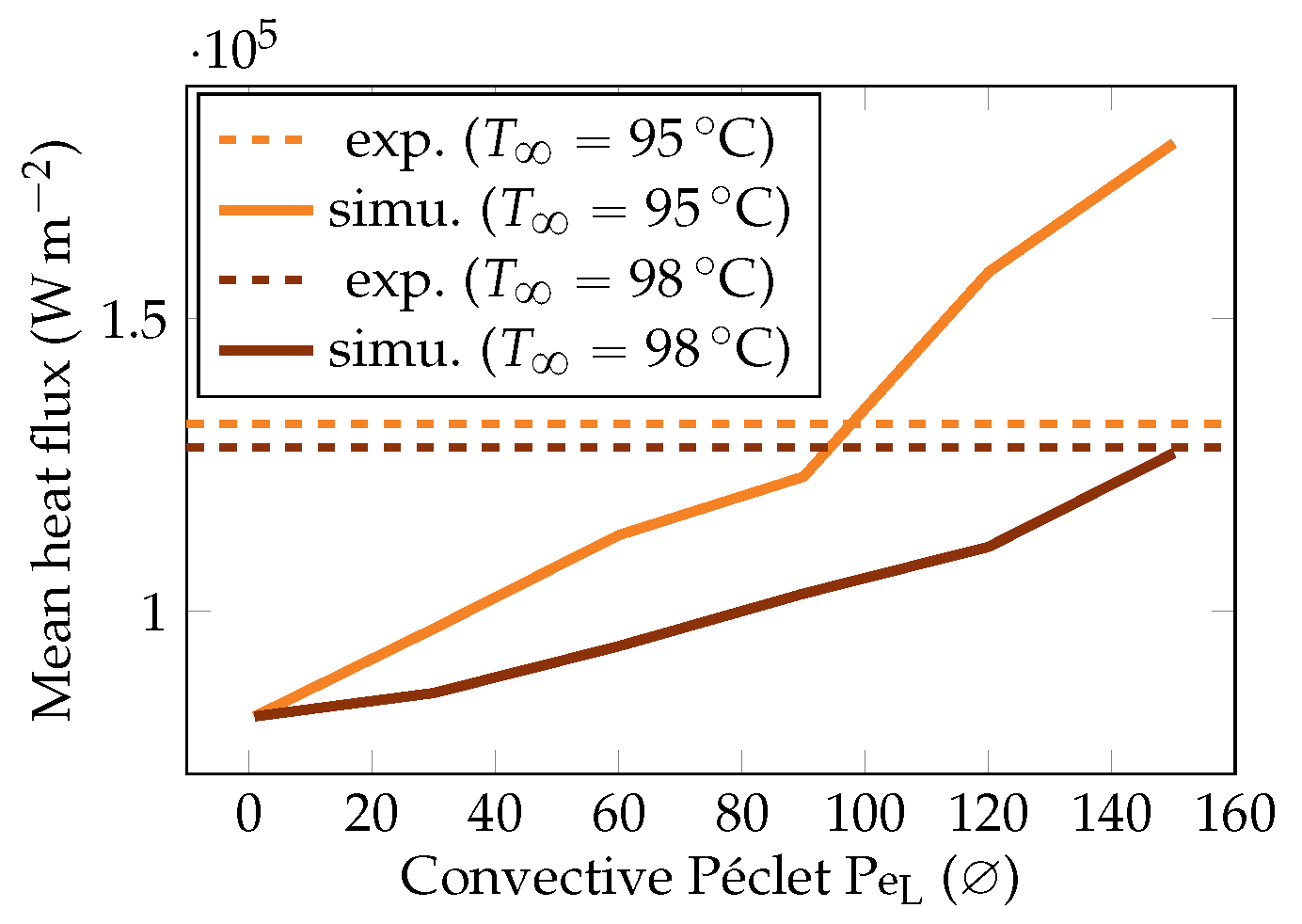
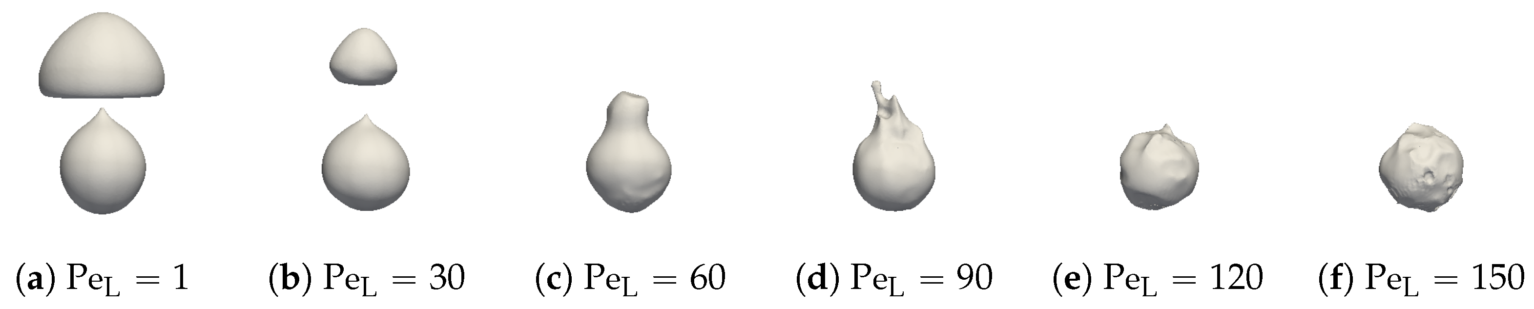
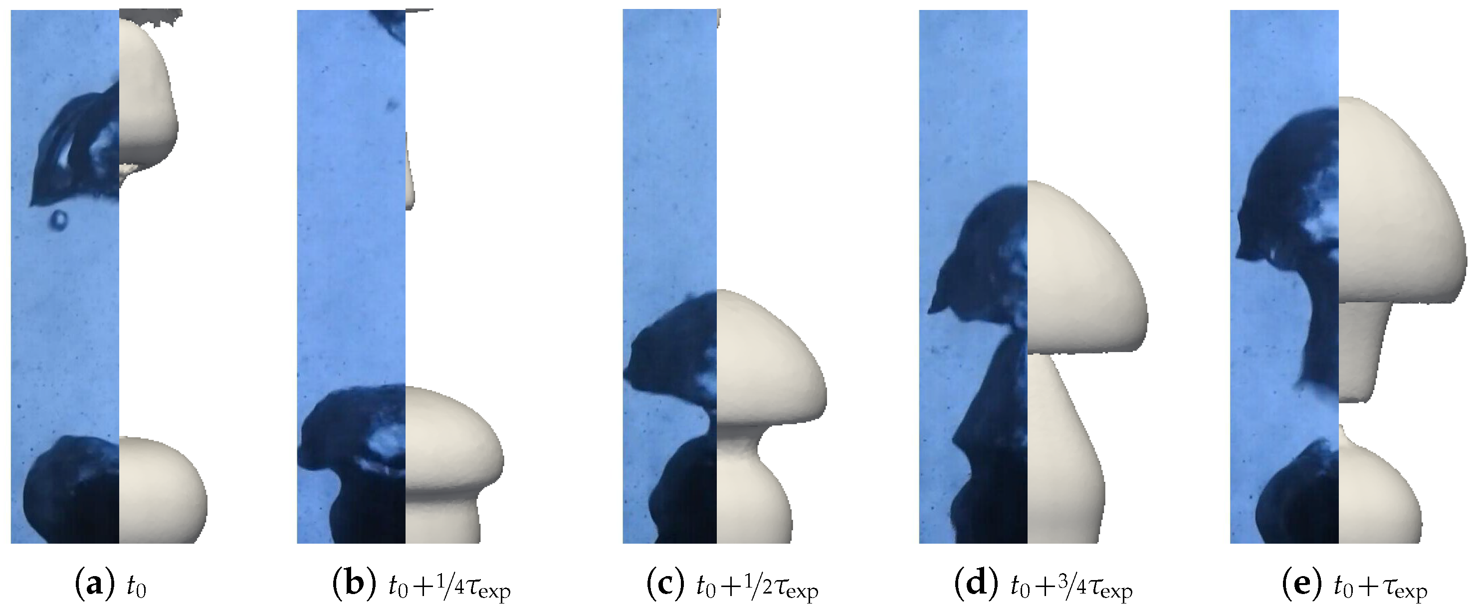
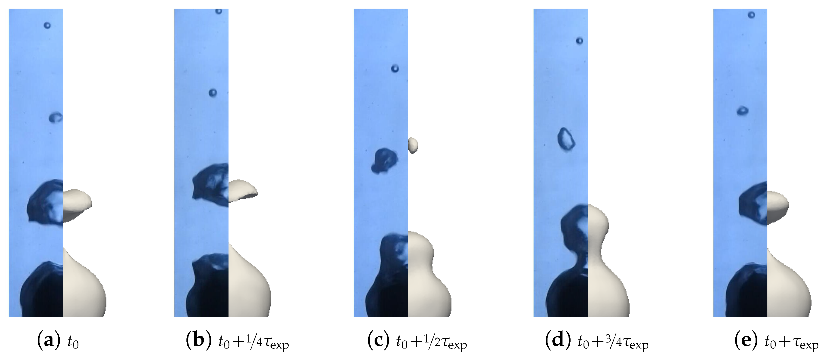

Disclaimer/Publisher’s Note: The statements, opinions and data contained in all publications are solely those of the individual author(s) and contributor(s) and not of MDPI and/or the editor(s). MDPI and/or the editor(s) disclaim responsibility for any injury to people or property resulting from any ideas, methods, instructions or products referred to in the content. |
© 2025 by the authors. Licensee MDPI, Basel, Switzerland. This article is an open access article distributed under the terms and conditions of the Creative Commons Attribution (CC BY) license (https://creativecommons.org/licenses/by/4.0/).