Abstract
This work presents a machine learning (ML) approach to volume-tracking for computational simulations of multiphase flow. It is an alternative to a commonly used procedure in the volume-of-fluid (VOF) method for volume tracking, in which the phase interfaces are reconstructed for flux calculation followed by volume advection. Bypassing the computationally expensive steps of interface reconstruction and flux calculation, the proposed ML approach performs volume advection in a single step, directly predicting the volume fractions at the next time step. The proposed ML function is two-dimensional and has eleven inputs. It was trained using MATLAB’s (R2021a) Deep Learning Toolbox with a grid search method to find an optimal neural network configuration. The performance of the ML function is assessed using canonical test cases, including translation, rotation, and vortex tests. The errors in the volume fraction fields obtained by the ML function are compared with those of the VOF method. In ideal conditions, the ML function speeds up the computations four times compared to the VOF method. However, in terms of overall robustness and accuracy, the VOF method remains superior. This study demonstrates the potential of applying ML methods to multiphase flow simulations while highlighting areas for further improvement.
1. Introduction
The VOF method uses a scalar indicator function, f defined by:
to represent a two-phase flow. On a discretized numerical grid, it is the fraction of the cell occupied by Fluid 1 defined by:
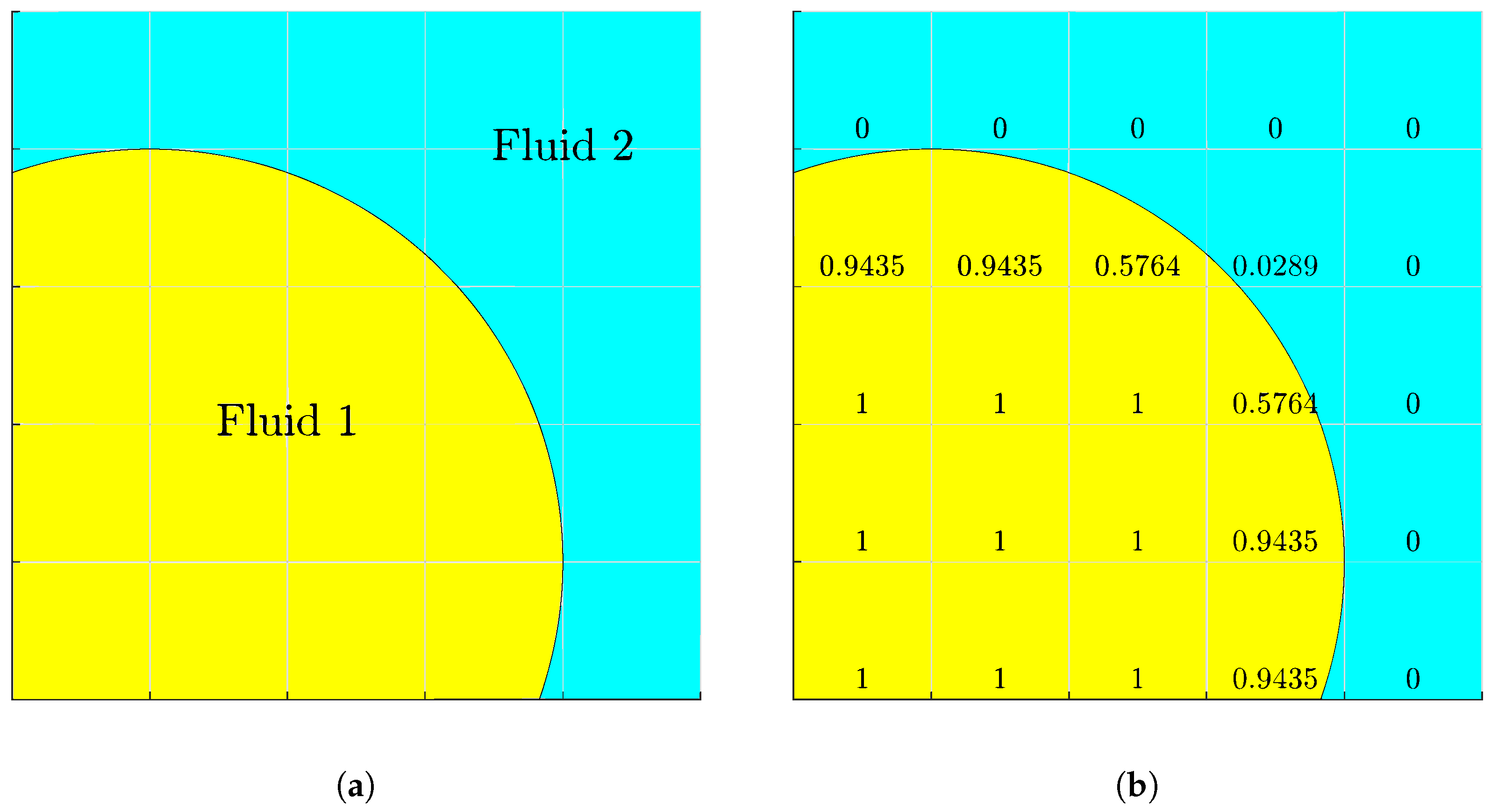
where V is the cell volume, and is discontinuous by nature. Fully occupied by fluid 1 is denoted as , completely void of fluid 1 as , and two-fluid or interfacial as , as depicted in Figure 1. The volume is tracked by the advection equation:

Figure 1.
(a) Two-phase interface. (b) Volume-of-fluid representation.
The most common solutions to the advection Equation (3) are geometric methods. Geometric methods follow a two-step process: interface reconstruction followed by flux calculation. Interface reconstruction uses a geometric approximation created from the F field. The simplest method is the simple line interface calculation (SLIC) method where, in a split manner, a straight line is constructed parallel to one of the coordinate axes. Only neighboring cells in the respective direction are needed. The fluxes are calculated from upwind and downwind cells with a weight determined by the orientation of the interface and local velocities. The simplicity of this method struggles with accurately capturing more complex configurations, and, as Noh and Woodward [1] observed, fluid separation for complex velocities when vorticities and shearing occur at the interface.
More commonly used is the piecewise linear interface calculation (PLIC) method where the equation of a line:
represents the interface. ensures that the volume under the interface is equivalent to the cell’s volume, and can be calculated in numerous ways. Youngs [2] used a straightforward method of the normalized gradient of F, but as the resolution increased, the accuracy reduced from second order to first order. Alternatively, a centered scheme using the neighboring row-wise or column-wise volume fractions for horizontal and vertical directions, respectively, can be used to calculate the slope. Pilloid and Puckett [3] presented the efficient least-squares volume-of-fluid interface reconstruction algorithm (ELVIRA) where six choices from forward, centered, and backward schemes are considered. The candidate that minimizes the least-squares error between the volume of the true and approximate interfaces is selected. ELVIRA is second-order accurate, but is computationally expensive. Scardovelli [4] combined the centered-column method and the least-squares approach of ELVIRA in least-square fit where a radius extends from the target cell and all points are used in a linear or quadratic least-square fit.
Once the interface is reconstructed, the volume fluxes are calculated in either a Lagrangian or Eulerian reference frame in a split or unsplit manner. Split methods are simpler by comparison. The volume is updated to an intermediate volume after a directional sweep and is updated to after all directions have been swept. The order of the direction sweeps changes with each iteration to prevent directional bias. In a Lagrangian frame, the endpoints of the reconstructed line segment are advected by local velocities. The volume that has moved across the cell face is the flux. In an Eulerian frame, the volume under the interface of width moves across the face determined by velocity.
Unsplit methods are more complex. In a Lagrangian frame, the vertices containing the fluid are advected by local velocities. This results in new polygons cut by the cell faces, and the volumes of the resulting polygons are distributed. In an Eulerian frame, the fluxed regions overlap and will be advected multiple times. Rider and Kothe [5] proposed cutting the corners with triangles based on the face center velocities forming a trapezoidal flux region that reduces but does not eliminate the overlap. López et al. [6] expanded on this by using cell vertex velocities to eliminate the overlap. López et al. [7] wrapped many of these methods into the VOFTools library.
Interest in the application of machine learning in computational simulations of multiphase flow has been increasing. Zhu et al. [8] provide a review of various ML implementations for improving the efficiency and accuracy of computational fluid dynamic (CFD) simulations of multiphase flow. The approaches range from simple neural networks (NNs) to data-driven surrogates. They point to extensive works utilizing ML algorithms for closure modeling for drag, turbulence, heat, and mass transport. Ma et al. [9] used data generated from direct numerical simulations (DNSs) of a simple bubble system to create a relatively small NN consisting of one hidden layer with 10 nodes. This NN was able to create a function for the closure terms of interest. When implemented and tested, the NN recovered the main aspects of the DNS solutions. Tang et al. [10] utilized ML as an alternative for determining the coefficient and correlation regarding bubble condensation. The resulting NN, consisting of three hidden layers with 80, 40, and 20 nodes in the layers, was trained on experimental data and randomly generated data points of existing conditional correlations. They found good agreement when compared to experimental data without the need to select the appropriate correlation and coefficient.
Ansari et al. [11,12] deployed data-driven surrogates in place of conventional CFD simulations. Their data sets were comprised of phase fraction, pressure, and velocity components produced by CFD and proposed three approaches: data from a single time step, multiple time steps from “significant dynamic moments”, and repeating the multiple time step approach with the addition of time steps with the highest error. The surrogates showed good agreement with the CFD solutions while being computationally less expensive. Similarly, Ganti and Khare [13] developed a framework for data-driven surrogates trained on DNS results utilizing the VOF method for flow over a circular cylinder and liquid injection in a quiescent environment. They noted excellent agreement between the DNS and surrogate solutions, as well as excellent speed up.
Several efforts have been made to incorporate ML into different aspects of the VOF method. One area is the calculation of interface curvature. Qi et al. [14] substituted conventional interface curvature calculations with a single hidden layer NN of 100 nodes. They proposed a relationship between the interface curvature and the volume fractions of a stencil for utilizing 2D circles of various sizes as their data set. Patel et al. [15] extended this to three-dimensions using a stencil of volume fractions. Their data set comprised 3D waves, ellipsoids, and Gaussian surfaces. They deploy a grid search method to find an optimal NN topology of a single hidden layer with 80 nodes. Both studies showed good agreement with analytical solutions and other curvature calculation methods. Cervone et al. [16] altered the inputs opting to use the height function instead of the volume fractions. They found an optimal size of a single hidden layer with 100 nodes. A key note in their study was that the NN lacked convergence with grid resolution compared to its conventional counterpart.
The ML work also includes the interface normal calculation and interface reconstruction. Li et al. [17] developed an NN to compute the interface normals in the VOF method in 3D. Much like the previous formulations, they showed that a relationship between the interface normals and the volume fractions of a stencil could be generated. The data set used spheres of various sizes, and the resulting NN consisted of three hidden layers with 50, 20, and 10 nodes, respectively. When compared to Young’s method and the height function for reconstruction, the NN produced lower errors for various test conditions. Ataei et al. [18] coined NPLIC, referring to using an NN for computing PLIC calculations. They proposed using separate NNs relating in Equation (4) to the inputs specific to the mesh type. Their NNs produced interface reconstruction results as accurate as conventional PLIC for a variety of mesh types, while providing up to five times speed up. Cahaly et al. [19] proposed an alternative formulation, referred to as PLIC-Net, for interface reconstruction using the volume fractions of stencil and the phasic barycenters. Their data set was compromised of various paraboloid surfaces to resemble common interface geometries observed in multiphase flows. The resulting NN used three hidden layers with 100 nodes in each layer. They reported improvements versus the least-squares volume-of-fluid interface reconstruction algorithm (LVIRA), and ELVIRA as PLIC-Net had fewer errors than LVIRA with only limited spurious planes and lower computational costs when implemented into a flow solver. Finally, Després and Jourdren [20] approached the dimensionless flux calculations in the VOF method via NN. Their data set was comprised of circles with the addition of corners to cover cases that could not be represented by a single line with increasing mesh resolution. They tested and stencils, noting that both exhibit roughly the same accuracy for smooth interfaces, but the stencil performed better for corners.
In this work, we present a data-driven approach, that is a ML function that directly calculates F of the next time step without the need for the typical two-step process. That is a novel application of ML to volume tracking in the VOF-based multiphase flow solvers. The structure of the papers is as follows. First, the problem setup and ML approach will be laid out. Then, the ML function’s performance will be evaluated on commonly used advection tests and a set of new tests. Finally, a discussion and summary will conclude the paper.
2. Machine Learning Methodology
2.1. Function Inputs
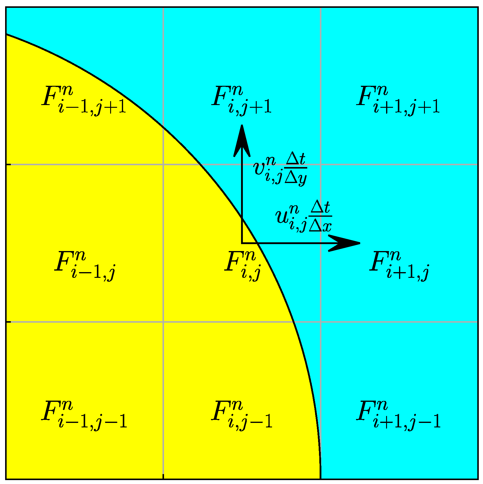
Consider the interface geometry and the underlying mesh shown in Figure 2, as an example, where the volume fractions in a stencil centered on a target cell are available at time step n. Of interest is the volume fraction of at the next time step , denoted by as a function of the volume fractions in the stencil and the velocity components located at the center of . Calling that function g, we write:
where the velocities were nondimensionalized using the mesh size in the respective direction, or , and the time step size, , which is the time interval between n and . The nondimensional velocities are the Courant numbers (CFL) in the x and y directions. Note that all the inputs to the function g are nondimensional.
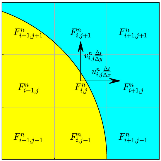
Figure 2.
Input stencil comprised of the target cell , its neighbors, and velocity components.
2.2. Data Generation
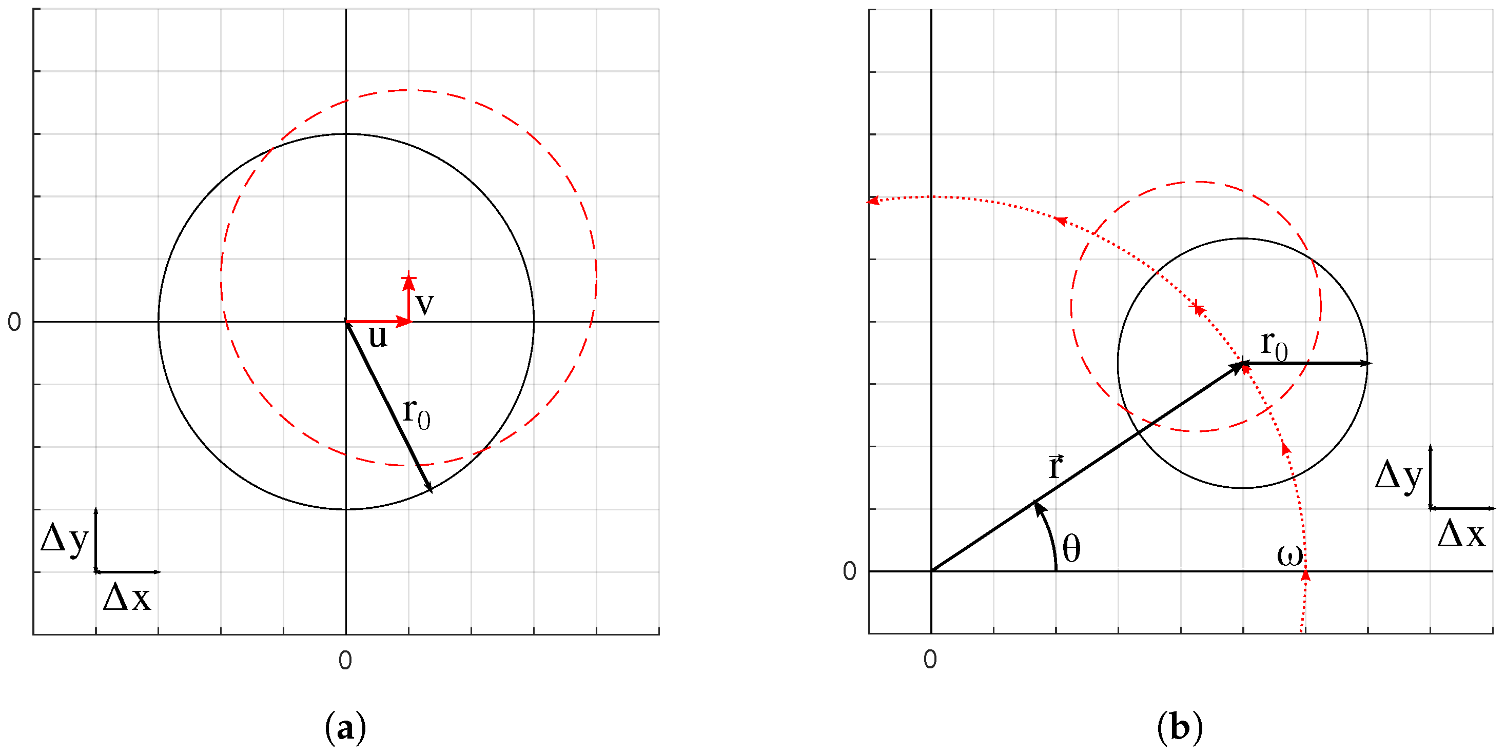
The data set was comprised of circles for two advection cases: translation and rotation. The translation velocity field was constant in both directions, while the rotation velocity field represents rigid-body rotation. The setups are depicted in Figure 3. Both cases follow a similar procedure. The F field of a circle centered at was initialized, referred to as the initial field. The circle center was advected one time step to , the location of which is determined by the nondimensional velocity components (or CFL defined earlier), and the F field was reinitialized at the new location, referred to as the final field. A marking function was implemented to identify and tag interfacial and near interface cells, where the F value has the potential to change as the circle is advected. The F values of the tagged cells were then considered as the inputs, and the corresponding F values of the final field were saved as the outputs. This single time step advection was repeated for various resolutions and CFL conditions.
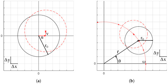
Figure 3.
Domain setups for (a) translation and (b) rotational data sets. Black is the initial position, and red is the new position.
To balance and expand the data, we also considered the reverse case, where the circle initially began at and was advected to by reversing the direction of the velocity field. Swapping the input and output fields, the final field was deemed as the inputs, and the initial field as the outputs. Additionally, the F field was inverted by setting the inverted F field to of the original field. Inverting was applied to the forward advection outlined in the previous paragraph and to the reverse process. The marking function was reapplied to the reversed and inverted processes to tag the correct cells. Finally, to further expand the data set in the rotation cases, the F fields were mapped to the other quadrants of the 2D coordinate system.
The resolution ranged from 2 to 40 cells per diameter (CPD) while using a square mesh such that . Velocity was bounded to be . This is dependent on the stability of the flow solver. The ML function’s stability was unknown. Typically, ML functions interpolate, and extrapolating could produce unexpected results. We tested the ML functions to perform both.
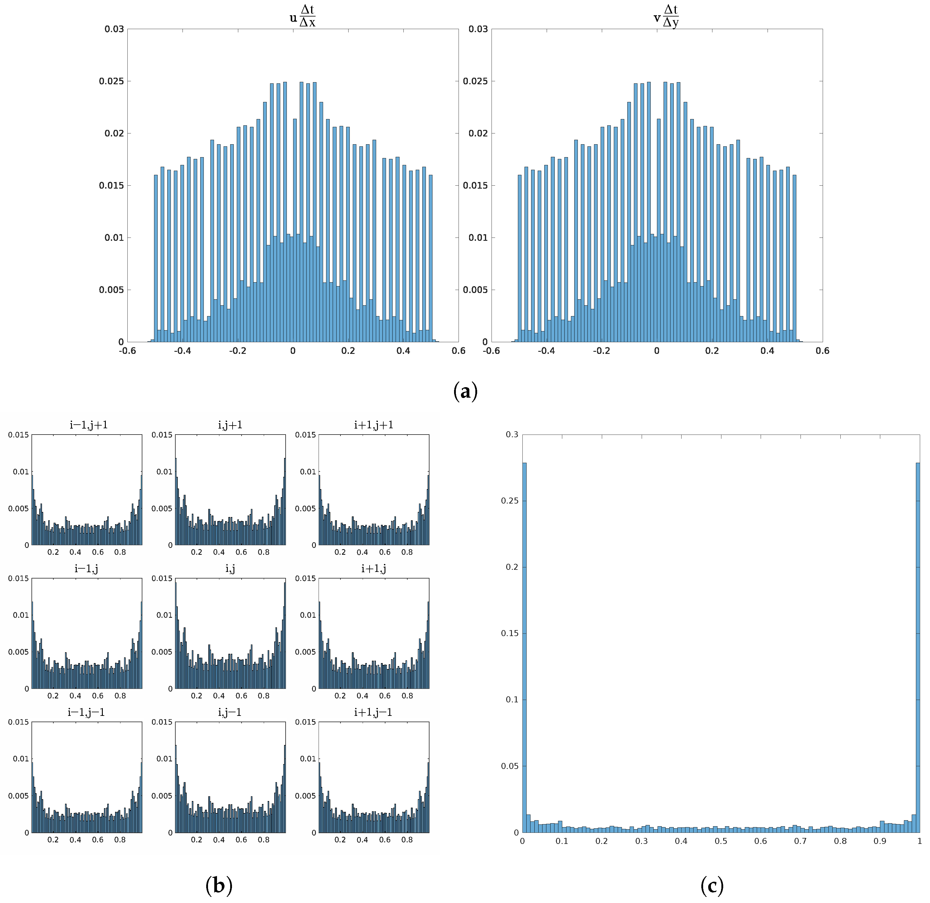
The full data set contained roughly data points. Translation and rotation consisted of and data points, respectively. Although not a 50:50 split, the data set had a good balance with the variety of input configurations. The distributions of values for inputs and outputs are presented in Figure 4. The spikes in Figure 4a are a result of discretizing the velocity spread as opposed to random selection. For the volume fractions, empty and full cells will inherently dominate the distribution as there are more near-interface cases than on the interface.

Figure 4.
Probability distributions for (a) non-dimensional velocity components, (b) input F, and (c) output F. Note that the bins for 0 and 1 are removed for the inputs in (b) as these values dominate the distribution and detract from the distribution of the other values. Including these gives a distribution similar to (c).
2.3. Model Training
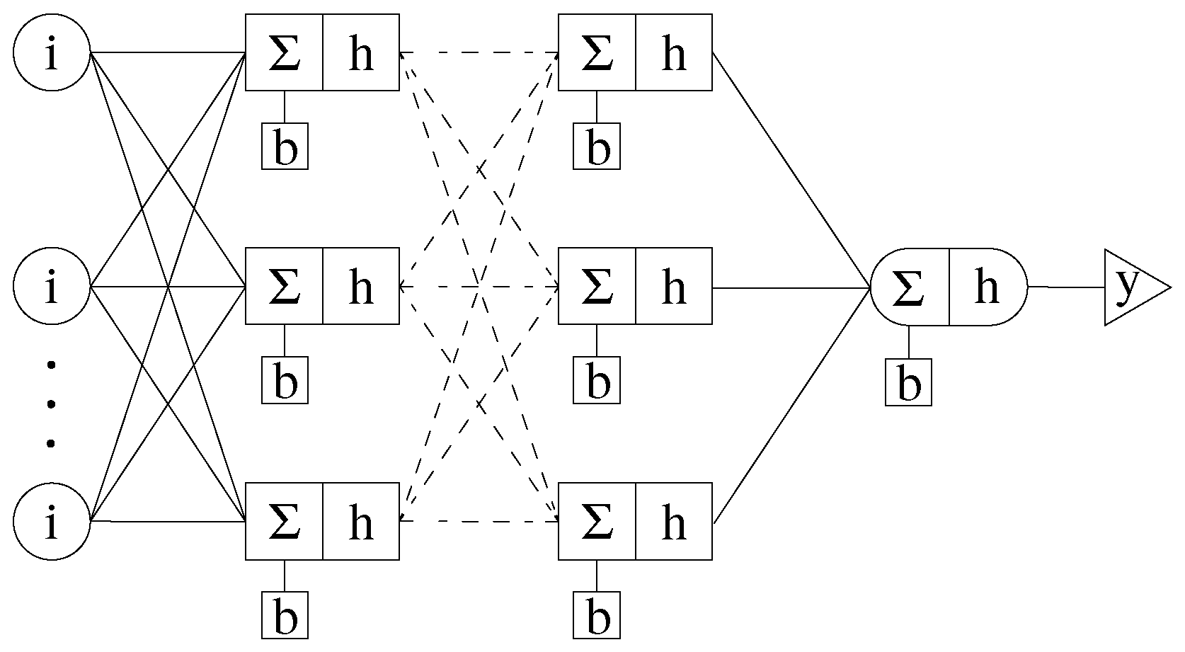
The data set was shuffled and divided into subsets using the typical split ratio of for training, for testing, and for validation. A fully-connected feedforward multi-layer perceptron (MLP), depicted in Figure 5, was used. The output y of an MLP’s layer is defined by:
where r is the number of nodes in the layer, h is an activation function, is the number inputs, are the weights, are the inputs, and b is the bias. In the first hidden layer, the inputs are the 11 inputs defined previously. The outputs of the first layer become the inputs of the next layer and so on. There will be one node in the output layer giving . The network’s topology, which is the number of hidden layers and nodes in each layer as the hyperparameters were to be determined.
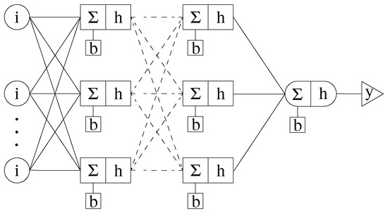
Figure 5.
Multi-layer perceptron (MLP) of arbitrary size resulting in one output.
A basic grid search method was deployed to search for an optimal network topology where the number of hidden layers ranged from 1 to 3 and each layer comprised 5, 10, 20, 50, or 100 nodes. A hyperbolic tangent is defined by:
was used for all activation functions. The weights were initialized using the Nguyen-Widrow algorithm [21], which has been shown to produce good results and reduce training time. There is a degree of randomness with this initialization. As such, the same seed was used for all training.
The weights were updated using the Levenberg–Marquardt algorithm for solving non-linear least squares problems [22,23]. Hagan and Menhaj [24] adapted the algorithm to a feedforward network. The algorithm is an adaptation of the Gauss–Newton method defined by:
where is the Jacobian matrix of network errors with respect to the weights. Typically, can be used to approximate the Hessian matrix and the second derivative does not need to be calculated. However, may not exist. To remedy this, the LM algorithm adds a term to give:
where I is the identity matrix, and shifts the algorithm between the steepest gradient descent with a small learning rate when it is large and Gauss–Newton when it is small. This gives the LM algorithm the ability to quickly search for the local minimum using the steepest gradient descent. Then, we can take advantage of Newton’s faster and more accurate capabilities closer to the minimum point [25].
The ML function was developed using MATLAB’s Deep Learning Toolbox train function [26] as it is streamlined and straightforward to use. The train function monitors the cost function for each data subset for each epoch, and stopping occurs when one of the following conditions is met:
- The maximum number of epochs is reached (1000 by default).
- The maximum specified wall time is reached (no limit by default).
- The performance goal is reached (0 by default).
- The validation performance fails to improve after a set number of consecutive epochs (6 by default).
- The minimum gradient is reached ( by default).
- The maximum value is reached ( by default). This is specific to the Levenberg–Marquardt algorithm.
Of these conditions, reaching the performance goal, the validation failure, or minimum gradient was the most desirable. Although desirable, reaching the performance goal was not likely. The minimum gradient was adjusted to , as some network training would end prematurely. Leaving the validation failure check as the goal. The train function ties validation performance and weight saving together as the final weights are pulled from the best epoch. If the performance fails to improve after subsequent epochs, the best weights are achieved. The performance was measured by the mean squared error (MSE) defined by:
where N is the data set size, t is the target value, and y is the NN output.
2.4. Training Results and Model Selection
To reduce excessive computation time, an initial round of training was performed utilizing a subset of data points. In addition to their validation performance, a small test and rating system were created to aid in network selection.
The test was comprised of a 10-by-10 domain where a 3-by-3 square of full cells were advected by the ML functions with for 4 time steps. The square starts aligned with the grid, and after four time steps, it was advected one cell length in both directions. The maximum error , the average error , and the percent volume error given by:
were calculated at the final time step between the exact and ML solution. The errors were not limited to the cells of interest and included the whole domain. The errors were combined with the validation performance to create the rating given by:
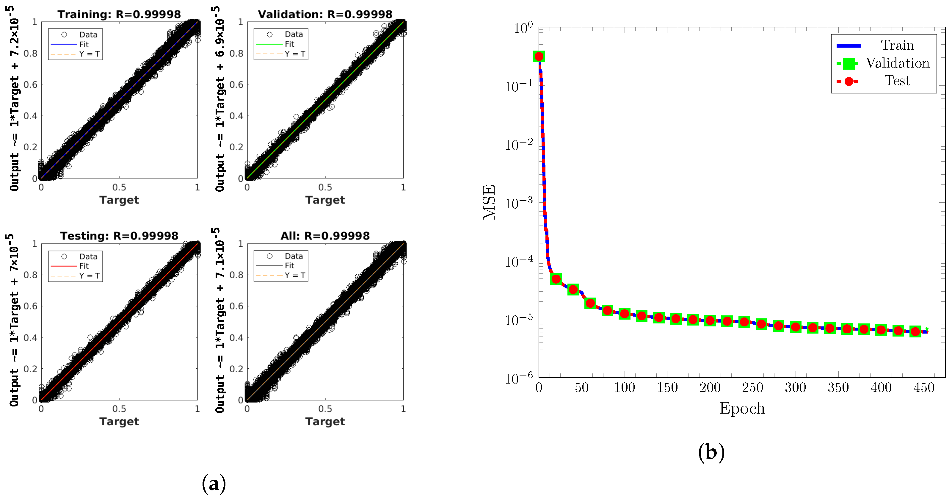
The training results for various configurations in the initial round of training are reported in Table 1. Generally speaking, deeper networks had better performance. Several configurations were selected for retraining on the full data set based on their rating and validation performance. The results of the second round are reported in Table 2. Because the rating system was unproven, all of the trained functions were subjected to the tests in the following section. A network configuration of three hidden layers comprising 100 nodes in the first layer, 10 in the second, and 10 in the third was chosen as the final topology based on its ability to complete and produce the lowest errors for the test cases presented in the following section. This model’s training results are shown in Figure 6. No major outliers were observed in the band around the line of perfect fit . In addition, the outputs were constrained to due to the hyperbolic tangent activation function on the output layer. The LM algorithm was observed well as the errors decreased quickly in the first 50 epochs before decreasing at a slower rate, then dropping once more before crawling to a stop. Overfitting and underfitting did not appear to occur as the MSE performance for training, testing, and validation do not stray far from each other. Several studies present similar MSE curves also utilizing MATLAB’s train function with the LM algorithm [15] or Python machine learning packages [17,18,19]. Overfitting or underfitting was not observed in those studies.

Table 1.
Initial training results using a smaller data set. The network configuration is denoted by the number of nodes in each layer separated by a “:”. For example, 50:5 refers to 50 nodes in the first hidden layer followed by 5 in the next.
Table 2.
Second round of training results on the full data set. The network configuration is denoted by the number of nodes in each layer separated by a “:”. For example, 50:5 refers to 50 nodes in the first hidden layer followed by 5 in the next.
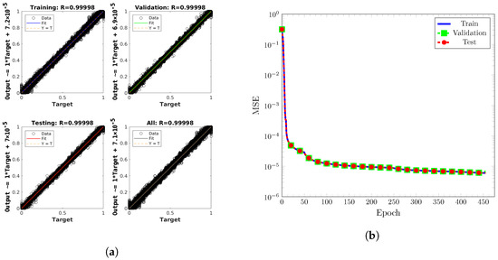
Figure 6.
Training results for network configuration of 100:10:10 on the full dataset. (a) Predicted ML values versus exact values. Plots generated by MATLAB’s plotregression. (b) MSE performances versus epoch.
3. Results
We present the results of the chosen ML function. It begins with a series of input sensitivity tests to gauge the ML function’s response to deviations in inputs and loosely relate the input contributions to the output. We follow with the 1D translation, rotation, and vortex test cases outlined in Raessi et al. [27] to provide a comparison between the ML function and other VOF methods. Additionally, a 2D translation test was added. A brief discussion of results specific to the tests will be provided here. More general discussions pertaining to all test cases will be made in the section after.
The same error metrics: , , and were used. Contour plots with levels at , , and will be displayed at points throughout the tests. For brevity, only the interface geometries from the ML function are presented here. The interface geometries associated with the other methods can be seen in [27] Two paths were tracked for translation and rotation cases: ML only and hybrid. ML only is self-explanatory where the volume fraction field is initialized at the starting position, and was advected by the ML function at every time step. The difference between the ML only and hybrid path was that the ML function never used its previously predicted outputs as inputs. The exact solution at each time step for the translation and rotation cases was known and was supplied to the ML function as inputs. That is, the F field was initialized and the ML function would produce outputs for the next time step based on the exact values. At the next time step, the F field was reinitialized, and the ML function would once again produce outputs based on the exact values. This would highlight cascading errors versus single time step errors. For these tests, the contour plots will us a “+” to mark the center of mass calculated by:
where is the cell center location, and a dashed line represents the exact path.
3.1. Volume Sensitivity and Cell Contribution
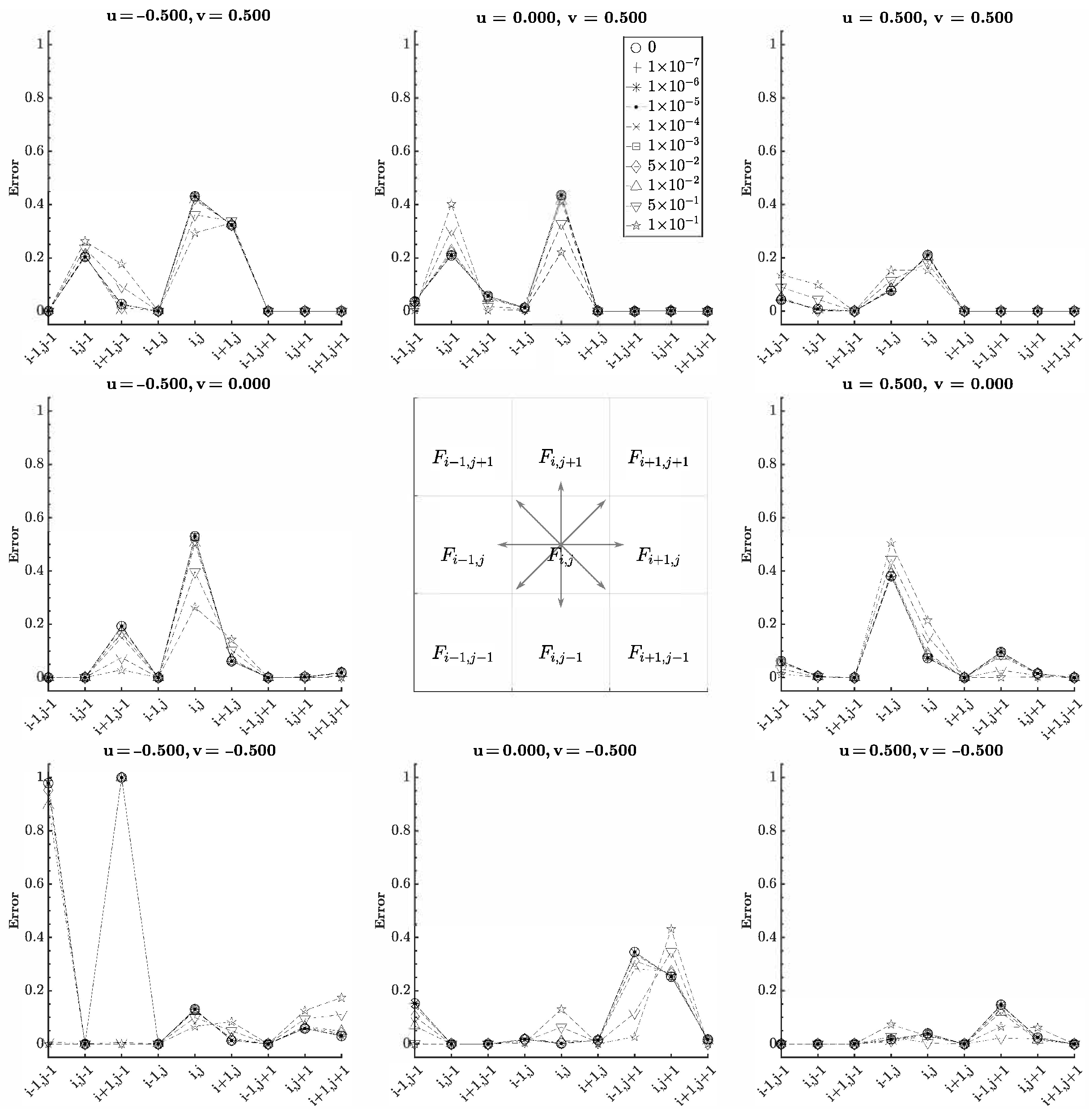
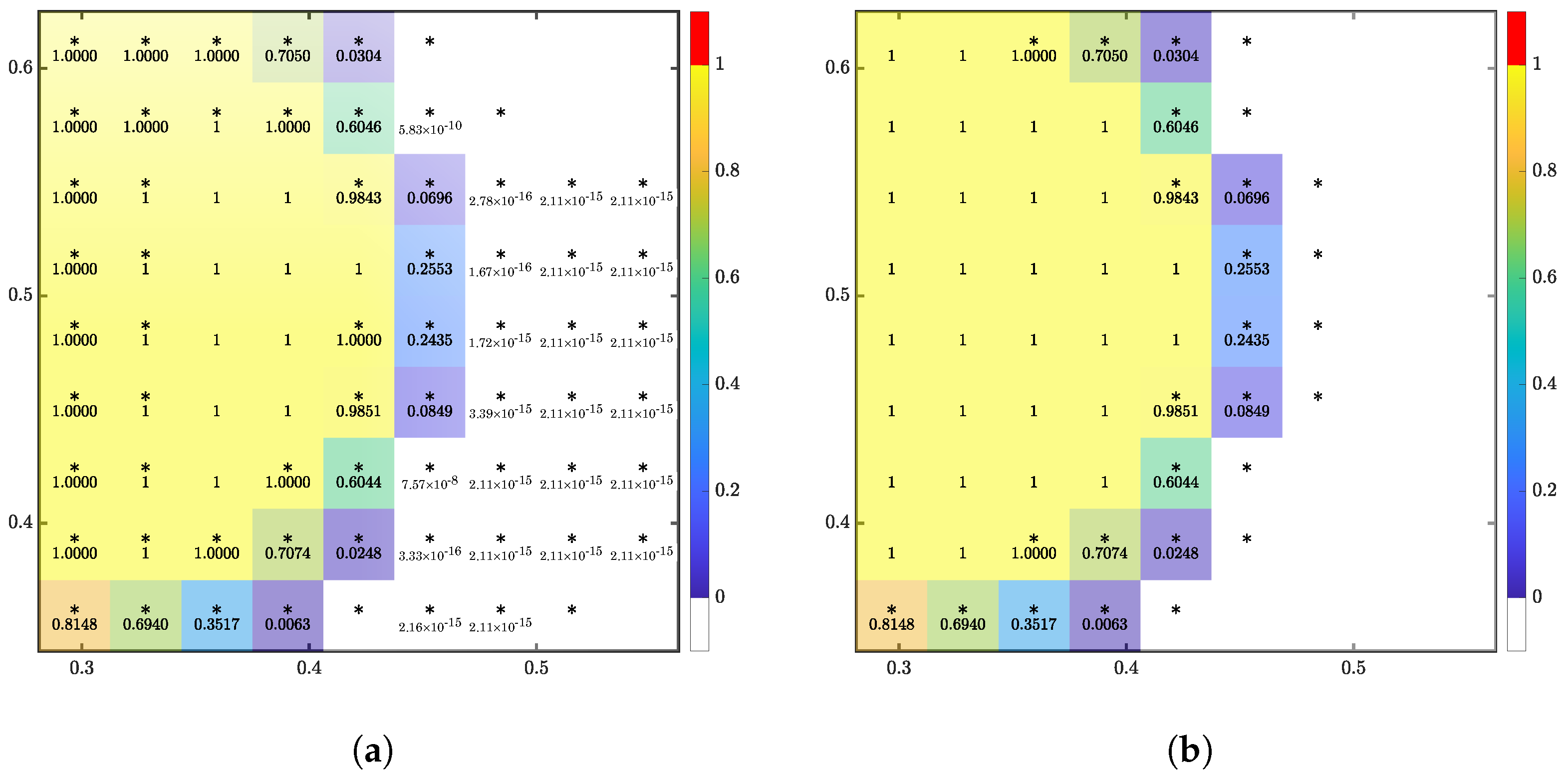
The purpose of this test was to determine the volume magnitude threshold in which the ML function becomes blind to values less than the threshold. Eight of the nine cells in the input stencil were initialized as full, and the last cell was variable. The location of the variable cell shifts through all of the input cell positions with a volume ranging from to . The value of the variable cell is referred to as the zero sensitivity value as the ML solution was compared to the exact solution when the variable cell was empty in each configuration. The results for in either direction are reported in Figure 7 and Figure 8. The volume threshold was found to be around ∼ evident by the relative error remaining constant until increasing or decreasing depending on the velocity and configuration.
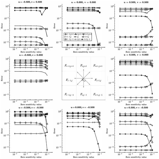
Figure 7.
Relative error for shifting variable cell position and variable cell value (zero sensitivity value) for . The input stencil is shown in the center and vectors correspond to the input velocity and error plot.
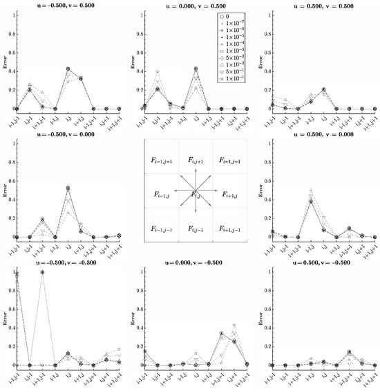
Figure 8.
Absolute error for shifting variable cell position and variable cell value (zero sensitivity value) for . The input stencil is shown in the center and vectors correspond to the input velocity and error plot.
Notice that the error depends on the position of the variable cell as well. This was the secondary purpose of the test—to provide insight into each cell’s contribution to the output. How the target cell donates and accepts fluid depends on the volume and velocity configuration. Consider translation in the positive x-direction. The target cell receives fluid from cell and donates fluid to cell . The other cells would have no effect on the target. Therefore, varying the volumes of the other cells would not change the output, and a constant error should be as they do not contribute to the target. Generally, this was observed. However, some exceptions can be observed in Figure 8. For , errors were observed when the value of corner cells and changed, similar to where corner cell produced error. Of particular note was , where cells and produced significant errors. Cell was expected as it receives fluid from the target. Cell was the outlier. As the cells became filled, the output was corrected.
3.2. Velocity Sensitivity
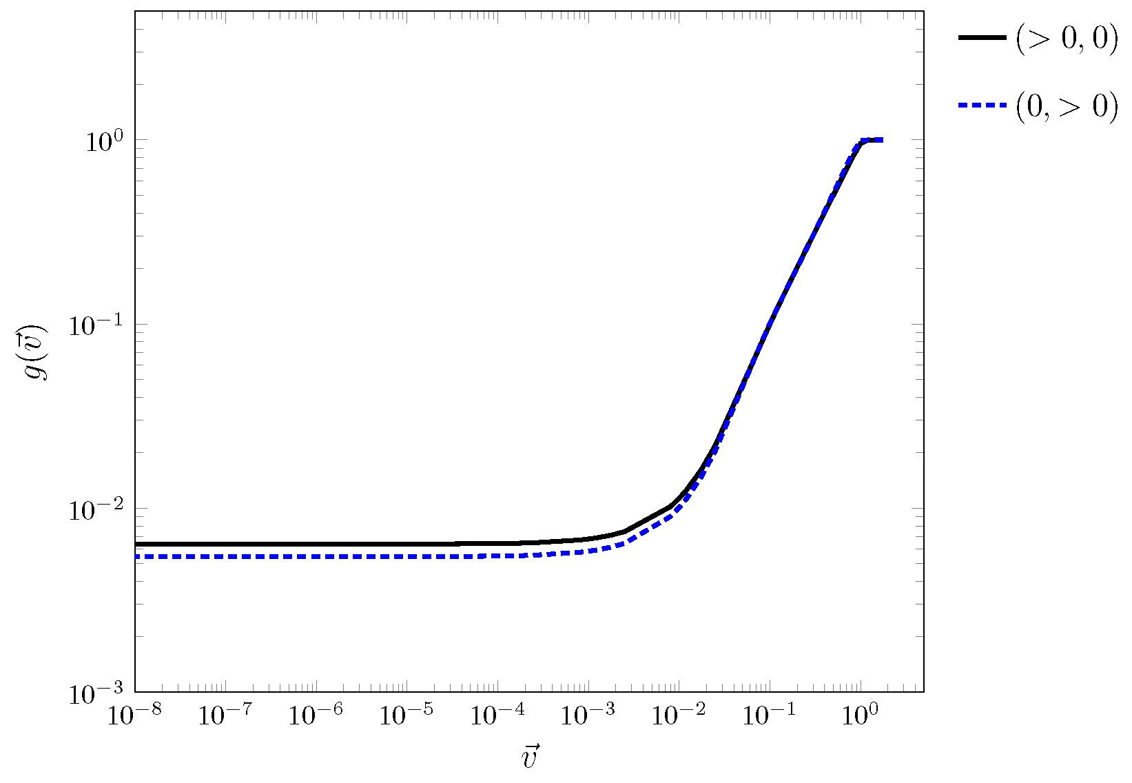
Similarly, the velocity inputs were expected to have a threshold. Three of the nine cells of the input stencil were initialized as full and the remaining were empty. The full cells were oriented such that they created occupied column for horizontal translation and row for vertical translation. The test varied the from to . The outputs of for varying magnitudes of are shown in Figure 9. Asymptotic behavior, as observed for the output and ∼, was determined to be the threshold. Coupling this with the volume sensitivity and cell contribution results, strange outputs with large errors for various input configurations were expected to occur.
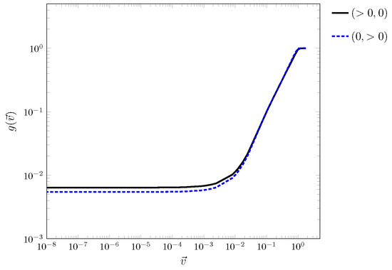
Figure 9.
for varying magnitudes of for pure horizontal and pure vertical translation.
3.3. Filter
The hyperbolic tangent activation constrained the output to asymptotically. When combined with floating-point numbers, the ML function rarely produced solutions of exactly zero or one. Outputs that should be unity were less of an issue compared to outputs that would be zero, referred to as residuals. Combining the residuals with the marking function, the residuals spread throughout the domain and eventually reached the computational bounds as depicted in Figure 10a. Based on several translation test cases, residuals were observed to infrequently peak around ∼ with this particular ML function.
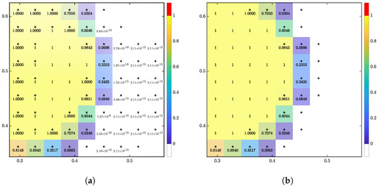
Figure 10.
The 1D translation for , after 6 time steps with filter strength (a) , and (b) . * indicates the cell is marked for the ML function. F values are displayed if the value is above 0. Perfect unity is represented by 1, and 1.0000 represents a rounding.
A filter was applied to correct the asymptotic values. For this ML function, filter strength was set to , one magnitude lower than the infrequently observed peaks. Tying in with the volume sensitivity results, volume inputs below had little to no impact on the ML output. With the filter applied, the residuals vanished, and the marked cells remained close to the interface, as depicted in Figure 10b.
3.4. The 1D Translation
A circle with radius 0.15 was initially centered at and was advected to in . A minimum velocity of , and a maximum of was used. Table 3 reports the errors between the ML only solution and the exact solution at the final position. Contour snapshots of the initial and final positions are shown in Figure 11. Error plots are shown in Figure 12, and final errors are reported in Table 3.
Table 3.
The 1D translation test errors. VOF and advecting normals conserve mass exactly.
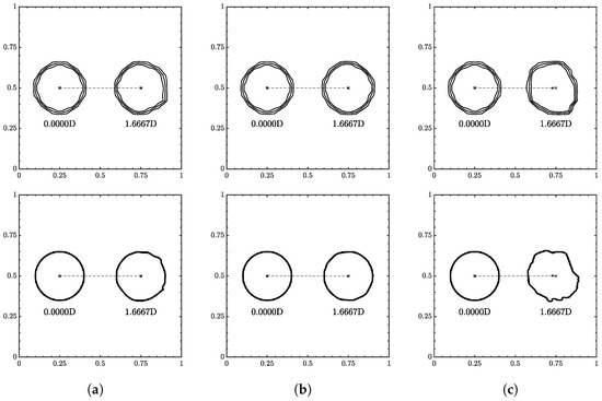
Figure 11.
Interface geometry for 1D translation for (a) , (b) , and (c) . Resolution of on top and on the bottom. Contour levels of , , and from outside in.
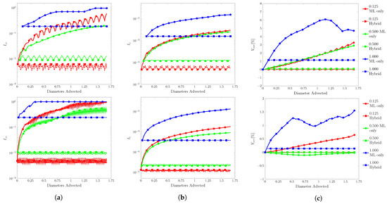
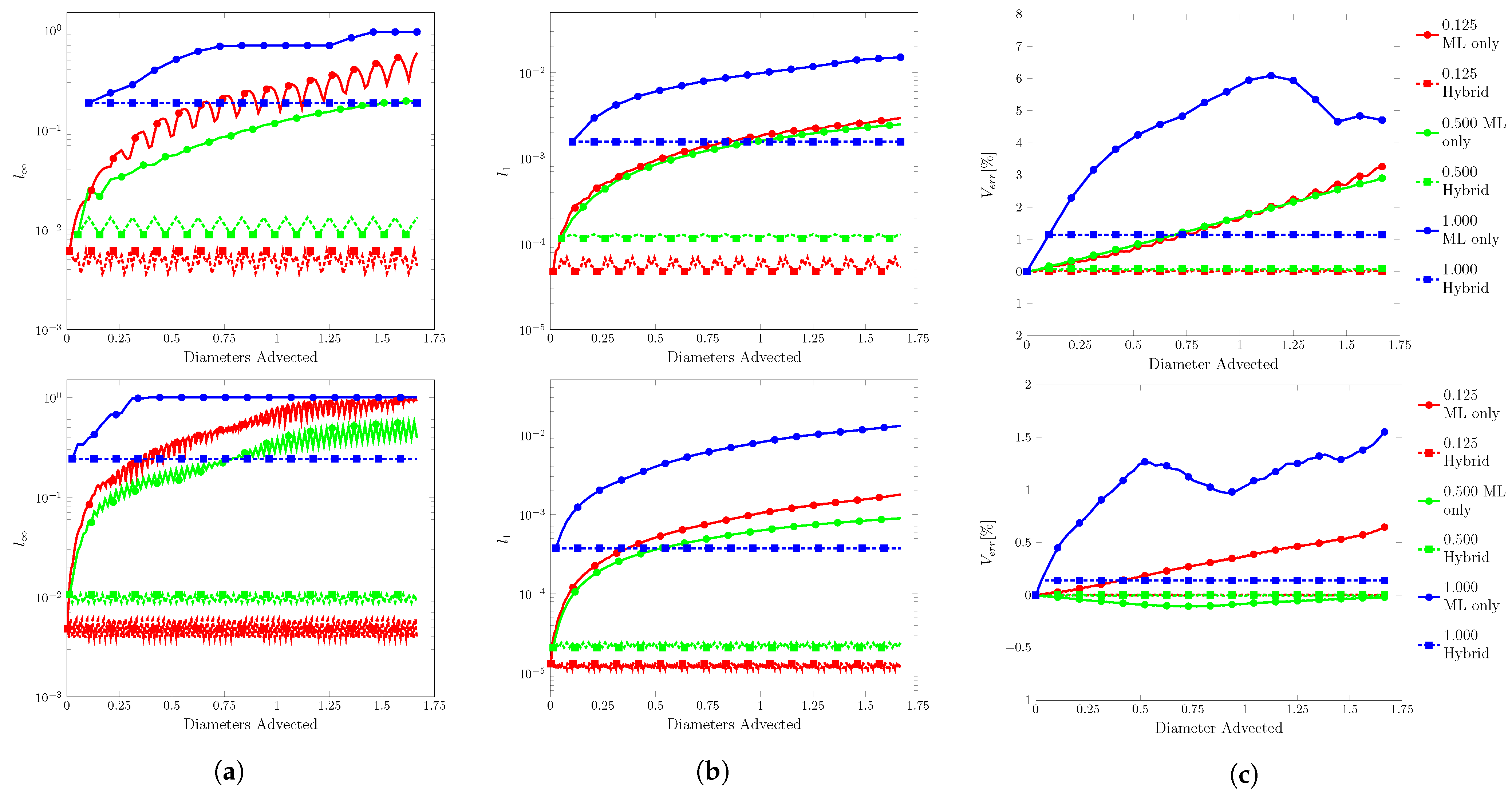
Figure 12.
Error plots for 1D translation. (a) , (b) and (c) . Resolution of on top and on the bottom.
There is not much to note here as the ML function was able to run at all velocity conditions and resolutions without fluid separation and minimum interface distortion. As increased, the overall shape appeared to flatten and interface distortions appeared most notably in the highest velocity cases.
3.5. The 2D Translation
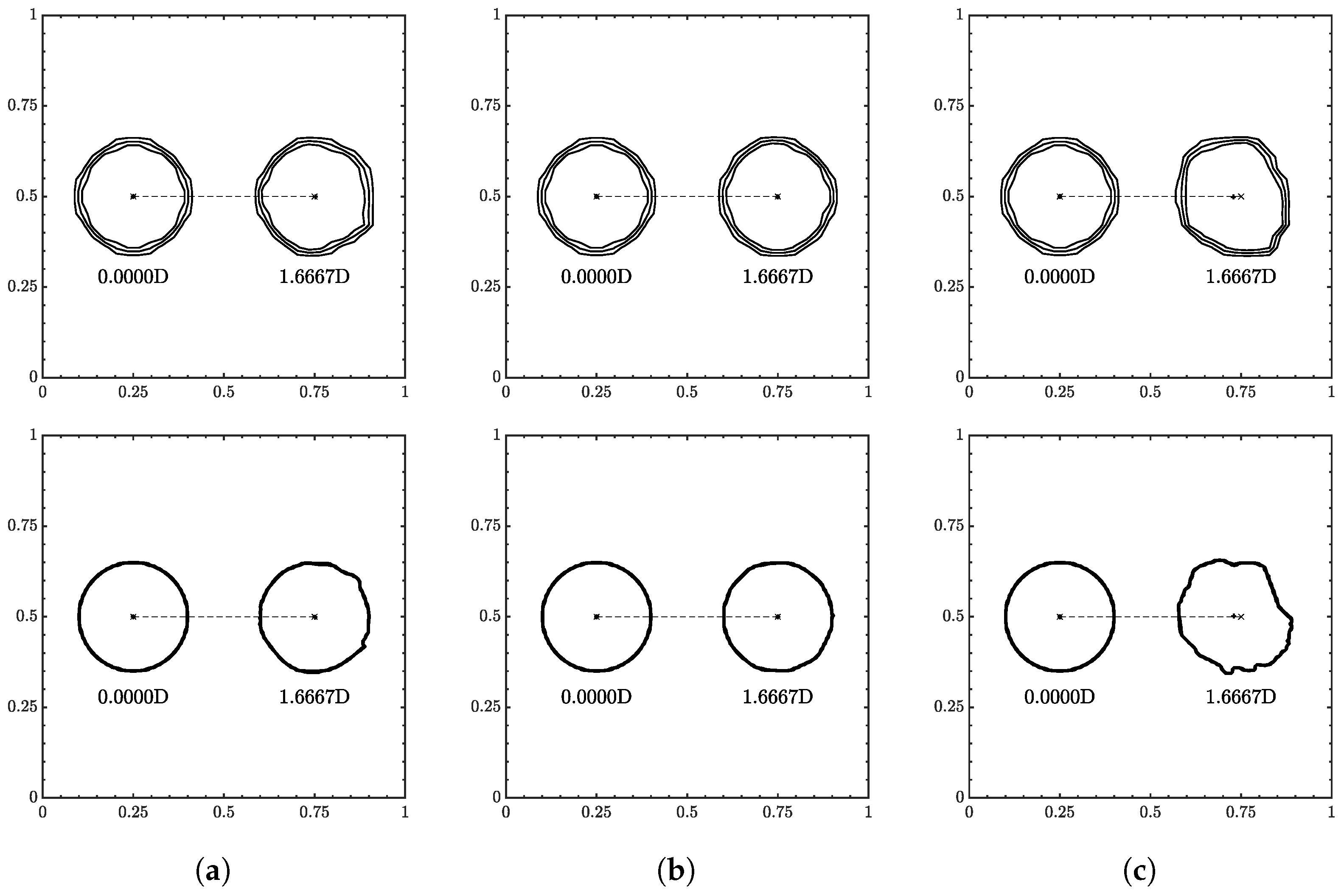
A circle of radius 0.15 was initially centered at and was advected to (0.75, 0.55) in . The velocity used the same range as the 1D translation test, and the velocity field had a ratio of . Contour snapshots of the initial and final positions are shown in Figure 13. Error plots are shown in Figure 14, and final errors are reported in Table 4.
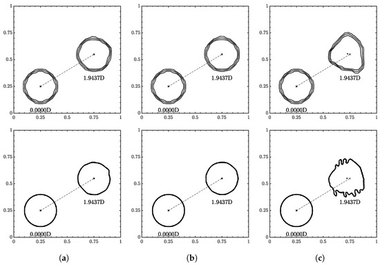
Figure 13.
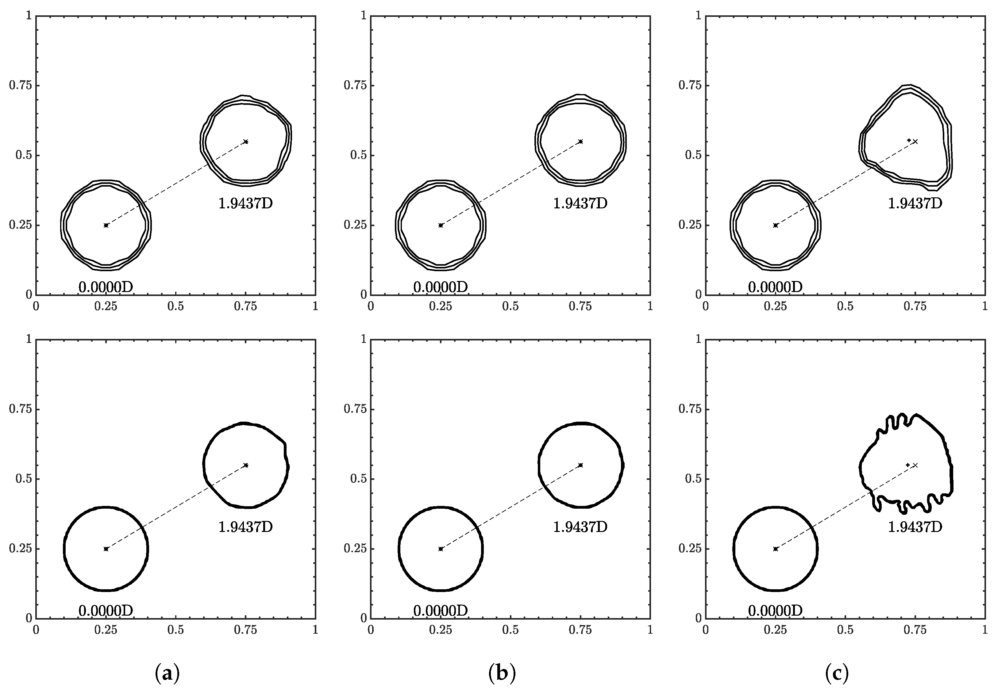
Interface geometry for 2D translation for (a) , (b) , and (c) . Resolution of on top and on the bottom. Contour levels of , , and from outside in.
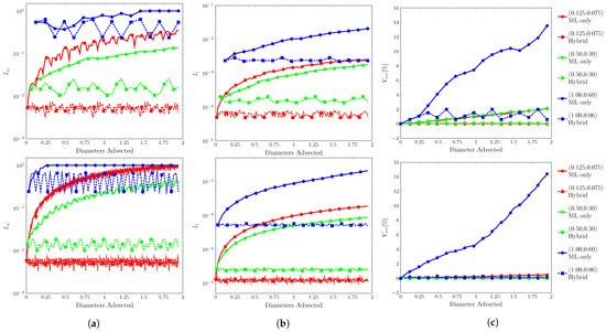
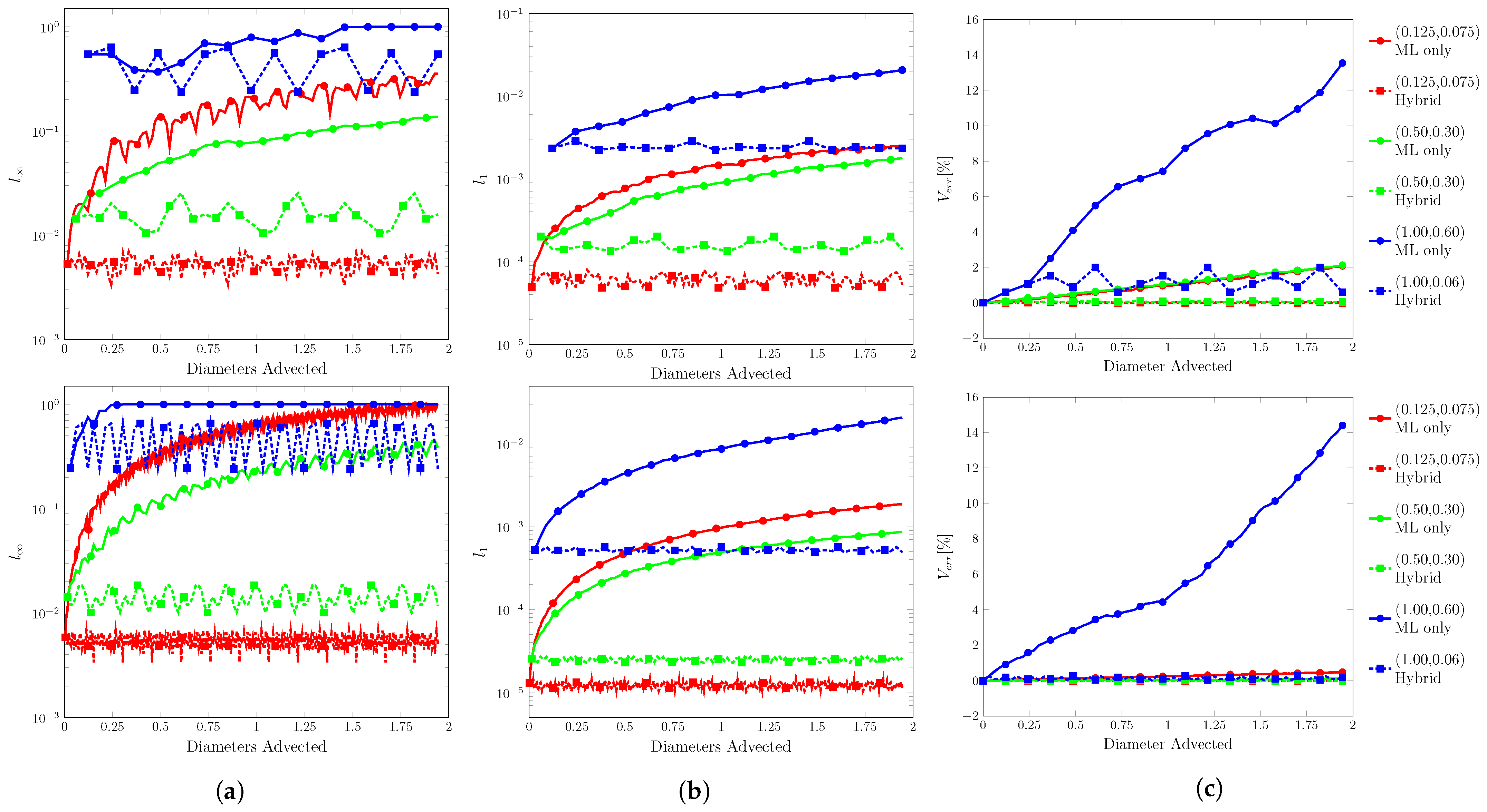
Figure 14.
Error plots for 2D translation. (a) , (b) , and (c) . Resolution of on top and on the bottom.
Table 4.
The 2D translation test errors.
Similar to 1D translation, the ML function was able to run all conditions without fluid separation. The interface flattening and distortions were more apparent at high-velocity conditions. Especially in where the contours appear more triangular at , and fingers/tendrils begin to appear at .
3.6. Rotation
A circle of radius 0.15 was initially centered at (0.75, 0.5) in . The center of rotation is (0.5, 0.5) with an angular velocity . ranged from to . Contour snapshots at every third of a revolution are shown in Figure 15. Error plots are shown in Figure 16, and the final errors are reported in Table 5. If the test exited prematurely, the final position is reported instead of the errors.

Figure 15.
Interface geometry for . (a) , (b) , (c) , and (d) . Resolution of on top and on the bottom. Contour levels of , , and from outside in. used to suppress residuals.

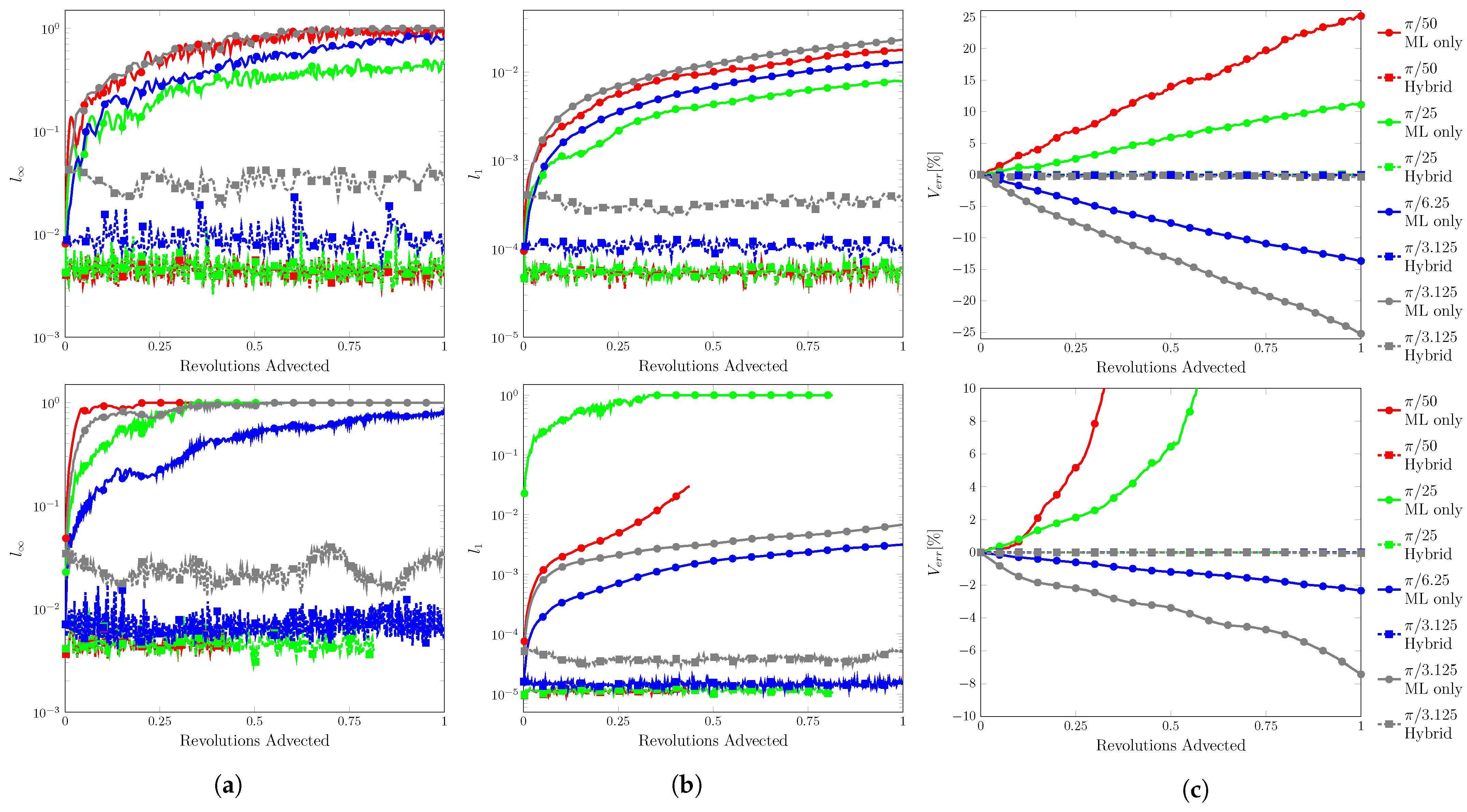
Figure 16.
Error plots for rotation. (a) , (b) , and (c) . Resolution of on top and on the bottom. used to suppress residuals.
Table 5.
Rotation test errors. VOF and advecting normals conserve mass exactly.
The ML function struggled at the lowest velocity condition, only completing the test at the lowest resolution. At the other resolutions, fluid separation was observed beginning on the edges closest to the domain bounds and at the center of the domain. The separations appeared to stick in place and continued to grow with proceeding time steps in the velocity direction. On the outer edge, the separations also grew to the domain bounds.
This unexpected behavior was due to the velocity inputs, as these issues were not observed when increased. In the prescribed velocity field, occurred at the domain bounds going to zero towards the domain center. The velocity inputs would be around ∼ on the outside edge and lower towards the domain center. As observed in the velocity sensitivity results, low to ∼ corresponded to transitioning to the threshold.
The best performance was seen from to with the ML function completing at all resolutions with no fluid separation. At , the filter strength needed to be increased to as residuals peaked around high ∼ at completion. These residuals spread to the domain bounds ending the test.
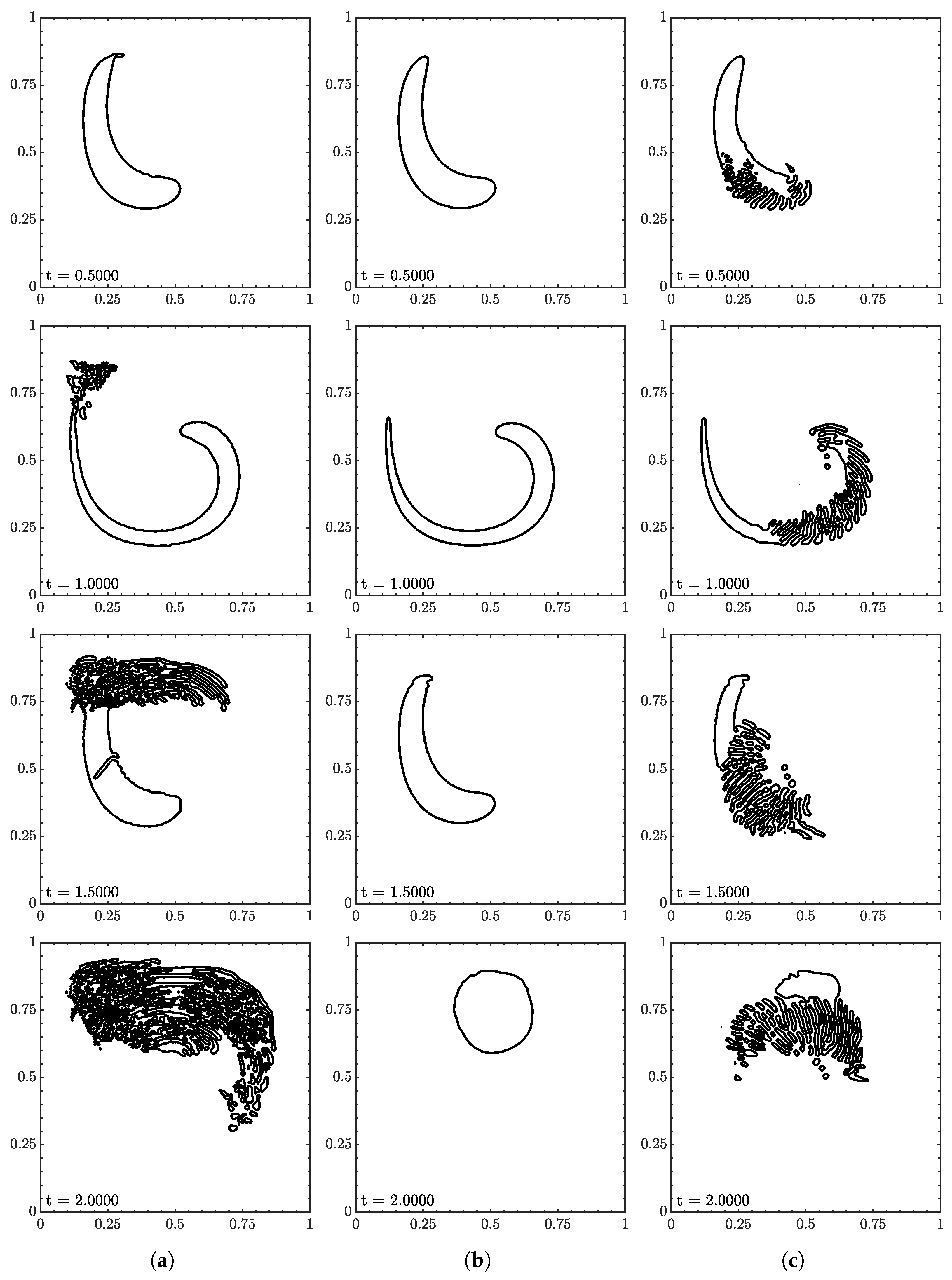
3.7. Vortex Test
A circle of radius 0.15 was initially centered at (0.5, 0.75) in . The velocity field was defined by:
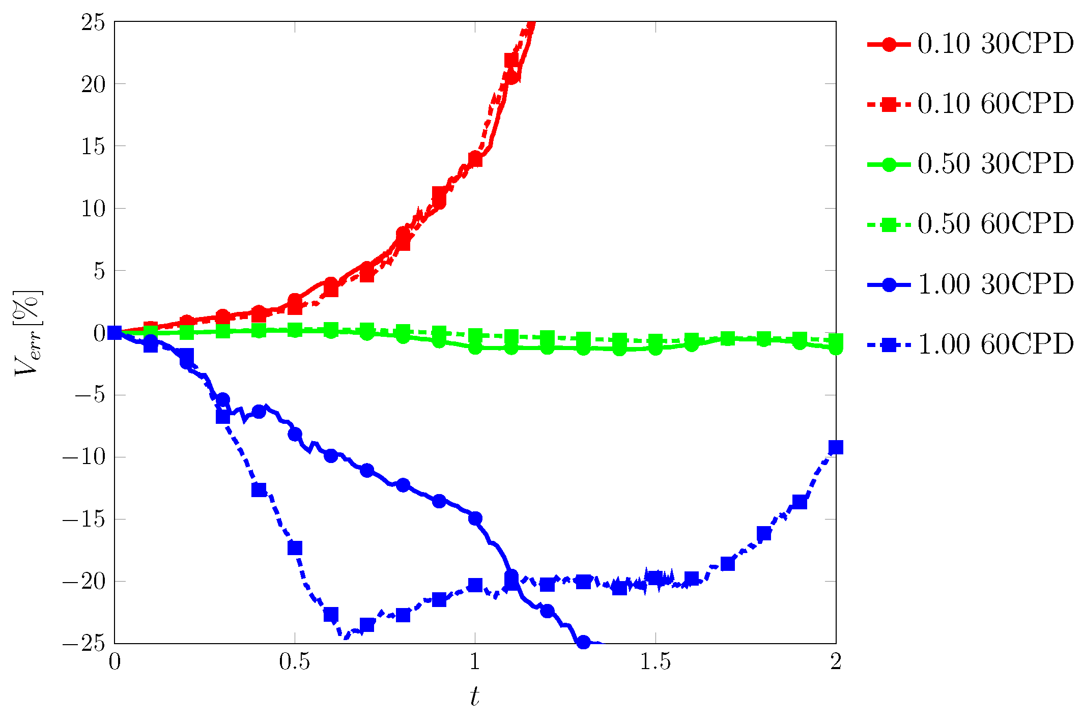
The fluid was advected to , the velocity was reversed and advected to where the fluid should return to its initial position, recovering its initial interface geometry, i.e., a circle of radius centered at . Contour snapshots at , , , and are shown in Figure 17 and Figure 18 for 30 and 60 CPD, respectively. Unlike the previous tests, the exact solution is only known at the initial and final positions. As a result, and of the volume fraction field could not be tracked throughout the test; they are only available at the end of the test () and are reported in Table 6. Throughout the vortex test (i.e., ), only the error in the total volume, , can be monitored, which is shown in Figure 19.
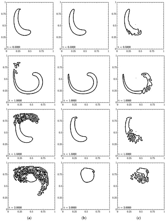
Figure 17.
Interface geometry for vortex test at (a) , (b) , and (c) at 30 CPD. Contour levels of , , and from outside in.

Figure 18.
Interface geometry for vortex test at (a) , (b) , and (c) at 60 CPD. Contour levels of , , and from outside in.
Table 6.
Vortex test errors. VOF and advecting normals conserve mass exactly.
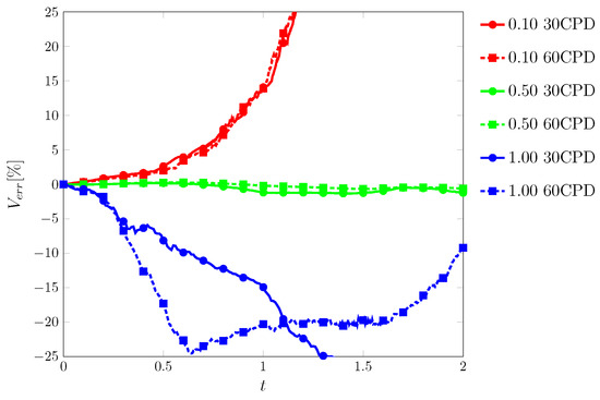
Figure 19.
Error in total volume, , as a function of time in the vortex test by the ML function for CFL numbers of , , and and mesh resolutions of 30 and 60 cells per diameter (CPD).
The ML function struggled the most with this test and was only able to complete it with specific conditions. The most consistent range was from to where the fluid returned to its original shape with minimum interface distortion, and volume was conserved well.
There appeared to be two different failure areas between low and high . At low the tail was the point of failure as it would separate multiple times. Rudman [28] reported similar behavior for other VOF methods on a similar test, a key difference being that the separations maintained a local shape in Rudman. Here, the separations spread like in the rotation test. In contrast to rotation, the separation growths closely follow the velocity field. The tail is a common point of failure due to its sharp interface. In terms of machine learning, the tail was not reflected in the data set, but one could argue the tail could be represented by a series of circles. One could also argue that the area was under-resolved, but no improvement was observed as the resolution increased. This pointed towards the velocity inputs where the range at a particular would produce unexpected results.
At , the leading portion was the problem area. This result was a surprise as this did not occur at other conditions. The leading and outer curve interfaces would begin to distort. At times, the leading curve would be first and vice-versa. The distortions would eventually split the body, growing with the velocity field. The velocity inputs are suspected to be the root again as this was more of a test of extrapolation compared to the translation and rotation tests.
4. Discussion
We begin with a discussion on resolution and error. Generally, when fell within the training data range, was inversely related to resolution. This was attributed to the number of time steps. In order to have a matching advection distance, the highest resolution required four times the amount of steps of the lowest resolution. The hybrid advection paths revealed that for single time steps produced a consistent range of error. With the ML only advection paths, the error would accumulate and invite more opportunities for unexpected outputs. It is likely that would reach its maximum given enough time steps. For CFL conditions above , begins relatively high, as extrapolations for velocity inputs were more prone to error.
The opposite was observed with and being directly related to resolution. This was attributed to the number of marked cells at any given time step. Recall that was defined as the average error in the domain, and the volume calculated by the sum of volume in all domain cells. Both of these metrics are heavily influenced by full and empty cells. Marked interface and near interface cells accounted for a small percentage of the total number of cells. Doubling the resolution resulted in a squared increase in the number of fluid cells, but only a doubling in marked cells. For the rotation test, marked cells represented , , and of the fluid cells for , , and , respectively. As resolution increased, the ML function had less effect on the domain.
Moving to the input values, the ML function was capable of completing all tests, but required certain conditions for the rotation and vortex test. For CFL conditions within the range of the training data, the ML function generally had little issue. As discussed previously, the struggles in the rotation and vortex tests at lower CFL were a result of the velocity inputs falling close to the threshold for velocity, and large errors were produced.
As CFL increased, performance improved until moving above where extrapolation with a high degree of uncertainty was required. For the ML function, it appeared that it had some capability to extrapolate in that the tests were completed. The translation tests began to exhibit interface deformations. More notably, in 2D translation, the shape was more deformed with protruding fingers. For rotation, although occurred at the domain bounds, the fluid was subjected to a velocity greater than on the outer edges and performed well. For the vortex test, the tail tip geometry required extrapolation and resulted in unexpected outputs. These errors then produced more strange outputs.
With these points stated, a major crux of the ML function was the unexpected outputs even under ideal conditions. In the volume sensitivity/cell contribution test, the volume configurations were relativity simple compared to the other tests, and the velocity inputs were within the training data range. Yet, large errors were produced. The outputs were accepted as the ML function cannot be easily modified. Attempting to find and adjust the weights responsible for the unexpected behavior would be daunting, especially for a network of this size. Additionally, this adjustment could propagate more errors throughout the network. It would be simpler to retrain the model on different data sets or different network configurations.
In comparison to the results of Raessi et al. [27], the ML function reported and one magnitude of order worse. The ML function did not conserve volume either, even though the data set was comprised of volume-conserving cases. At best, was less than , mostly due to the increased resolution. For other successful tests, reached . In terms of speed up, ML VOF completed the 1D translation test at in sub 30 s. Raessi et al. [27] reported VOF and advecting normals at 2 min and 13 min, respectively. Note that it is not a perfect comparison with the differences in hardware and program environment with Raessi et al. [27] utilizing C.
For future work, there are a plethora of directions. A natural progression would be the extension to 3D. This comes with the challenge of producing a dataset that sufficiently represents the range of inputs. Another avenue would be to adjust the data set to include different geometries and CFL conditions. Training on more geometries, such as sharp interfaces, might help resolve the tail in the vortex test. With CFL conditions, a wide range was attempted here. A wider range could be attempted with , or a specific range could be chosen based on the stability of particular flow solvers. To aid with network selection, a more robust rating system to better quantify the performance of a network could be developed. The rating system here was briefly mentioned, as limited success was found here as several ML functions were tested to find the “best” performing one.
Of the multitude of directions, creating more specialized functions and physics-informed neural networks are of particular interest. The general function could handle a variety of cases adequately. A combination of several specialized functions assigned to specific cases could improve the overall performance. A few examples include the following: one function to handle interface cells, and another to handle near interface cells. Since these are more specialized, the data sets and network configurations could be smaller, leading to faster training.
Another suggested future direction to potentially enhance the performance of the ML model for VOF advection is following the physics-informed neural networks (PINNs) approach introduced by Raissi et al. [29], which incorporates the underlying physical laws into the training process. Cai et al. [30,31] found success with the PINN approach when implemented in convective heat transfer, 3D wake flows, supersonic flows, and biomedical flows. Cuomo et al.’s [32] review points to additional implementations and modified formulations of the PINN approach to unsteady diffusion and advection. In this work, the advection (or transport) Equation (3), obtained through the conservation of mass law, governs the volume transport of multiphase flows. As such, using a PINN approach with the advection Equation (3) in the training process could lead to a mass-conserving function. Although the current approach uses volume (or mass) conserving data, that property is not perfectly preserved during training, pointing out the proposed PINN approach as a way to enforce mass conservation, thereby enhancing the ML model’s performance.
5. Conclusions
This work provides an outline for a machine learning approach to volume tracking. A marker function was developed to identify cells fitting the criteria of interfacial or near interfacial. A data set was generated using the advection of circles in translation and rotation cases with a variety of spatial and temporal resolutions, where data points were grabbed with the marker function. MATLAB’s train function from the Deep Learning Toolbox was utilized for its ease of use. A grid search method was deployed on a smaller subset to ease computation costs. A rating system was created to provide an additional metric for choosing a configuration instead of solely relying on the validation performance. Select configurations were then retrained on the full data set. The final function was chosen based on its performance on advection tests. A series of sensitivity tests were developed to gauge the response to subtle changes in the inputs and to show appropriate contributions. The results of these tests showed the thresholds in the inputs where unexpected results would be expected. A post-processing filter was used to reduce issues with the marker function and floating-point numbers. Its strength was determined from the results of the sensitivity tests. Translation and rotation resulted in consistent results working with a wide range of conditions including extrapolating at higher and resolutions not included in the training data. Vortex was the most difficult and required a narrow band of test conditions for successful tests. In comparison to Raessi et al. [27], the ML function produced higher errors and did not conserve volume. However, it yielded a four-times speed up compared to the VOF method and an even greater speed up compared to advecting normals. As noted previously, these were not direct comparisons with the differences in program environment and hardware.
Author Contributions
Conceptualization, M.R.; methodology, A.M. and M.R.; software, A.M. and M.R.; validation, A.M. and M.R.; formal analysis, A.M. and M.R.; investigation, A.M. and M.R.; resources, M.R.; data curation, A.M.; writing—original draft preparation, A.M.; writing—review and editing, M.R.; visualization, A.M.; supervision, M.R.; project administration, M.R.; funding acquisition, M.R. All authors have read and agreed to the published version of the manuscript.
Funding
This research was partially funded by UMass Dartmouth’s Center for Scientific Computing and Data Science Research.
Data Availability Statement
The original contributions presented in the study are included in the article; further inquiries can be directed to the corresponding author.
Acknowledgments
The computations were performed on the HPC cluster of UMass Dartmouth’s Center for Scientific Computing and Data Science Research. Special thanks to Ming Shao for providing assistance with regard to machine learning. We also thank Gretar Tryggvason for many fruitful discussions.
Conflicts of Interest
The authors declare no conflicts of interest. The funders had no role in the design of the study; in the collection, analyses, or interpretation of data; in the writing of the manuscript; or in the decision to publish the results.
References
- Noh, W.F.; Woodward, P. SLIC (Simple Line Interface Calculation). In Proceedings of the Fifth International Conference on Numerical Methods in Fluid Dynamics, Twente University, Enschede, The Netherlands, 28 June–2 July 1976; Springer: Berlin/Heidelberg, Germany, 1976; Volume 59, pp. 330–340. [Google Scholar] [CrossRef]
- Youngs, D. An Interface Tracking Method for a 3D Eulerian Hydrodynamics Code. At. Weapons Res. Establ. (AWRE) Tech. Rep. 1984, 44, 35. [Google Scholar]
- Pilliod, J.E.; Puckett, E.G. Second-Order Accurate Volume-of-Fluid Algorithms for Tracking Material Interfaces. J. Comput. Phys. 2004, 199, 465–502. [Google Scholar] [CrossRef]
- Scardovelli, R.; Zaleski, S. Interface Reconstruction with Least-Square Fit and Split Eulerian-Lagrangian Advection. Int. J. Numer. Methods Fluids 2003, 41, 251–274. [Google Scholar] [CrossRef]
- Rider, W.J.; Kothe, D.B. Reconstructing Volume Tracking. J. Comput. Phys. 1998, 141, 112–152. [Google Scholar] [CrossRef]
- López, J.; Hernández, J.; Gómez, P.; Faura, F. A Volume of Fluid Method Based on Multidimensional Advection and Spline Interface Reconstruction. J. Comput. Phys. 2004, 195, 718–742. [Google Scholar] [CrossRef]
- López, J.; Hernández, J.; Gómez, P.; Faura, F. VOFTools—A Software Package of Calculation Tools for Volume of Fluid Methods Using General Convex Grids. Comput. Phys. Commun. 2018, 223, 45–54. [Google Scholar] [CrossRef]
- Zhu, L.T.; Chen, X.Z.; Ouyang, B.; Yan, W.C.; Lei, H.; Chen, Z.; Luo, Z.H. Review of Machine Learning for Hydrodynamics, Transport, and Reactions in Multiphase Flows and Reactors. Ind. Eng. Chem. Res. 2022, 61, 9901–9949. [Google Scholar] [CrossRef]
- Ma, M.; Lu, J.; Tryggvason, G. Using Statistical Learning to Close Two-Fluid Multiphase Flow Equations for a Simple Bubbly System. Phys. Fluids 2015, 27, 092101. [Google Scholar] [CrossRef]
- Tang, J.; Liu, H.; Du, M.; Yang, W.; Sun, L. A Machine-Learning Based Phase Change Model for Simulation of Bubble Condensation. Int. J. Heat Mass Transf. 2021, 178, 121620. [Google Scholar] [CrossRef]
- Ansari, A.; Mohaghegh, S.D.; Shahnam, M.; Dietiker, J. Modeling Average Pressure and Volume Fraction of a Fluidized Bed Using Data-Driven Smart Proxy. Fluids 2019, 4, 123. [Google Scholar] [CrossRef]
- Ansari, A.; Boosari, S.S.; Mohaghegh, S.D. Successful Implementation of Artificial Intelligence and Machine Learning in Multiphase Flow Smart Proxy Modeling: Two Case Studies of Gas-Liquid and Gas-Solid CFD Models. J. Pet. Environ. Biotechnol. 2020, 11, 8. [Google Scholar] [CrossRef]
- Ganti, H.; Khare, P. Data-Driven Surrogate Modeling of Multiphase Flows Using Machine Learning Techniques. Comput. Fluids 2020, 211, 104626. [Google Scholar] [CrossRef]
- Qi, Y.; Lu, J.; Scardovelli, R.; Zaleski, S.; Tryggvason, G. Computing Curvature for Volume of Fluid Methods Using Machine Learning. J. Comput. Phys. 2019, 377, 155–161. [Google Scholar] [CrossRef]
- Patel, H.; Panda, A.; Kuipers, J.; Peters, E. Computing Interface Curvature from Volume Fractions: A Machine Learning Approach. Comput. Fluids 2019, 193, 104263. [Google Scholar] [CrossRef]
- Cervone, A.; Manservisi, S.; Scardovelli, R.; Sirotti, L. Computing Interface Curvature from Height Functions Using Machine Learning with a Symmetry-Preserving Approach for Two-Phase Simulations. Energies 2024, 17, 3674. [Google Scholar] [CrossRef]
- Li, J.; Liu, J.; Li, K.; Zhang, S.; Xu, W.; Zhuang, D.; Zhan, L.; Chen, Y. Three Dimensional Interface Normal Prediction for Volume-of-Fluid Method Using Artificial Neural Network. Eur. J. Mech.-B/Fluids 2024, 106, 13–20. [Google Scholar] [CrossRef]
- Ataei, M.; Bussmann, M.; Shaayegan, V.; Costa, F.; Han, S.; Park, C.B. NPLIC: A Machine Learning Approach to Piecewise Linear Interface Construction. Comput. Fluids 2021, 223, 104950. [Google Scholar] [CrossRef]
- Cahaly, A.; Evrard, F.; Desjardins, O. PLIC-Net: A Machine Learning Approach for 3D Interface Reconstruction in Volume of Fluid Methods. Int. J. Multiph. Flow 2024, 178, 104888. [Google Scholar] [CrossRef]
- Després, B.; Jourdren, H. Machine Learning Design of Volume of Fluid Schemes for Compressible Flows. J. Comput. Phys. 2020, 408, 109275. [Google Scholar] [CrossRef]
- Nguyen, D.; Widrow, B. Improving the Learning Speed of 2-Layer Neural Networks by Choosing Initial Values of the Adaptive Weights. In Proceedings of the 1990 IJCNN International Joint Conference on Neural Networks, San Diego, CA, USA, 17–21 June 1990; Volume 3, pp. 21–26. [Google Scholar] [CrossRef]
- Levenberg, K. A Method for the Solution of Certain Non-Linear Problems in Least Squares. Quart. Appl. Math. 1944, 2, 164–168. [Google Scholar] [CrossRef]
- Marquardt, D. An Algorithm for Least-Squares Estimation of Nonlinear Parameters. J. Soc. Ind. Appl. Math. 1963, 11, 431–441. [Google Scholar] [CrossRef]
- Hagan, M.T.; Menhaj, M.B. Training Feedforward Networks with the Marquardt Algorithm. IEEE Trans. Neural Netw. 1994, 5, 989–993. [Google Scholar] [CrossRef]
- Hagan, M.T.; Demuth, H.B.; Beale, M.H.; De Jésus, O. Neural Network Design, 2nd ed.; Martin T. Hagan: Stillwater, OK, USA, 2014. [Google Scholar]
- MATLAB, Version 9.10.0 (R2021a); The MathWorks Inc.: Natick, MA, USA, 2021.
- Raessi, M.; Mostaghimi, J.; Bussmann, M. Advecting Normal Vectors: A New Method for Calculating Interface Normals and Curvatures When Modeling Two-Phase Flows. J. Comput. Phys. 2007, 226, 774–797. [Google Scholar] [CrossRef]
- Rudman, M. Volume-Tracking Methods for Interfacial Flow Calculations. Int. J. Numer. Meth. Fluids 1997, 24, 671–691. [Google Scholar] [CrossRef]
- Raissi, M.; Perdikaris, P.; Karniadakis, G. Physics-Informed Neural Networks: A Deep Learning Framework for Solving Forward and Inverse Problems Involving Nonlinear Partial Differential Equations. J. Comput. Phys. 2019, 378, 686–707. [Google Scholar] [CrossRef]
- Cai, S.; Mao, Z.; Wang, Z.; Yin, M.; Karniadakis, G.E. Physics-Informed Neural Networks (PINNs) for Fluid Mechanics: A Review. arXiv 2021, arXiv:2105.09506. [Google Scholar] [CrossRef]
- Cai, S.; Wang, Z.; Wang, S.; Perdikaris, P.; Karniadakis, G.E. Physics-Informed Neural Networks for Heat Transfer Problems. J. Heat Transf. 2021, 143, 060801. [Google Scholar] [CrossRef]
- Cuomo, S.; Di Cola, V.S.; Giampaolo, F.; Rozza, G.; Raissi, M.; Piccialli, F. Scientific Machine Learning Through Physics–Informed Neural Networks: Where We Are and What’s Next. J. Sci. Comput. 2022, 92, 88. [Google Scholar] [CrossRef]


Disclaimer/Publisher’s Note: The statements, opinions and data contained in all publications are solely those of the individual author(s) and contributor(s) and not of MDPI and/or the editor(s). MDPI and/or the editor(s) disclaim responsibility for any injury to people or property resulting from any ideas, methods, instructions or products referred to in the content. |
© 2025 by the authors. Licensee MDPI, Basel, Switzerland. This article is an open access article distributed under the terms and conditions of the Creative Commons Attribution (CC BY) license (https://creativecommons.org/licenses/by/4.0/).