Vertical Dense Jets in Crossflows: A Preliminary Study with Lattice Boltzmann Methods

Abstract

The dramatic increase in domestic and industrial waste over recent centuries has significantly polluted water bodies, threatening aquatic life and human activities such as drinking, recreation, and commerce. Understanding pollutant dispersion is essential for designing effective waste management systems, employing both experimental and computational techniques. Among Computational Fluid Dynamics (CFD) techniques, the Lattice Boltzmann Method (LBM) has emerged as a novel approach based on a discretized Boltzmann equation. The versatility and parallelization capability of this method makes it particularly attractive for fluid dynamics simulations using high-performance computing. Motivated by its successful application across various scientific disciplines, this study explores the potential of LBM to model pollutant mixing and dilution from outfalls into surface water bodies, focusing specifically on vertical dense jets in crossflow (JICF), a key scenario for the diffusion of brine from desalination plants. A full-LBM scheme is employed to model both the hydrodynamics and the transport of the saline concentration field, and Large Eddy Simulations (LES) are employed in the framework of LBM to reduce computational costs typically associated with turbulence modeling, together with a recursive regularization procedure for the collision operator to achieve greater stability. Several key aspects of vertical dense JICF are considered. The simulations successfully capture general flow characteristics corresponding to jets with varying crossflow parameter $u_{r}F$ and most of the typical vortical structures associated with JICF. Relevant quantities such as the terminal rise height, the impact distance, the dilution at the terminal rise height, and the dilution at the impact point are compared with experimental results and semi-empirical relations. The results show a systematic underestimation of these quantities, but the key trends are successfully captured, highlighting LBM’s promise as a tool for simulating wastewater dispersion in aquatic environments.

1. Introduction

The rapid global growth in population and industrial activities has significantly increased the discharge of wastewater into natural water bodies, causing detrimental effects on aquatic ecosystems and human reliance on water for drinking, recreation, and economic activities, as well as increasing the potential for health risks [1,2]. Among the main sources of these discharges are desalination plants, which can harm marine life and disrupt the delicate balance in aquatic ecosystems. Effective management of coastal water quality requires the design of efficient wastewater outfall systems, which, in turn, depends on the study of pollutant dispersion and dilution. In fact, this implies understanding the characteristics of jets in crossflows (JICF)—streams of effluent discharged into a non-stagnant receiving ambient flow.

Studies focusing on JICF are very diverse in scope, as they represent a key fluid dynamics problem with numerous applications, particularly in aerodynamics and flow control: recent advances have demonstrated the effectiveness of pulsed JICF for controlling flow separation on airfoils [3] and for modulating momentum and frequency to enhance aerodynamic performance [4,5]. JICF also plays a prominent role in film cooling for gas turbine blades and fuel atomization in scramjets [6]. General overviews on JICF dynamics and supersonic jet injection into the water further underscore the wide relevance of this topic [7,8,9].

In the context of wastewater outfalls, JICFs are crucial in the dilution and dispersion of pollutants. Density differences between the effluent and the receiving water body are often involved, such as in the case of discharges of heated cooling water from power plants (positively buoyant jet) or brine from desalination plants (negatively buoyant jet) [10,11].

The mixing of effluents and characteristics of JICF can be investigated both through experimental and numerical means. Among the latter, Computational Fluid Dynamics (CFD) methods based on the discretization of the Navier–Stokes (NS) equations have been widely applied to simulate pollutant dispersion [12,13,14,15,16], thanks to advancements in technology and the availability of computational power. These approaches, however, often prove to be resource-intensive; thus, it is important to take full advantage of multi-core processors in boosting performance through parallel computations. The advent of High-Performance Computing (HPC) and multi-core architectures has encouraged the exploration of more efficient approaches, increasing performance and avoiding potential bottlenecks that can hinder the advantages of parallel execution. In this regard, Lattice Boltzmann Methods (LBM) are particularly well-suited, as the algorithm they employ is based on discretizing the Boltzmann equation rather than the traditional NS equation. This characteristic offers several advantages, chief among them a reduced communication footprint between processes, which is a major factor in fully harnessing the benefits of parallelization [17]. This is a key aspect in a post-exascale world, where numerical applications can leverage a vast number of processing units. For this reason, researchers from a wide range of disciplines involving fluid dynamics have begun exploring the range of applicability of LBM. Several studies have been conducted in the field of microfluidics [18], as well as in active fluids [19]. In general, LBM has evolved to tackle several problems, such as multiphase flows, with the color gradient method being successfully applied to simulate complex two-phase systems [20] and extensions incorporating heat transfer phenomena, further broadening its scope [21]. Comprehensive reviews highlight the growing multidisciplinary applications of LBM, including its use in acoustics [22] and nuclear engineering [23] and advection-diffusion models such as Mason–Weaver for sedimentation studies [24].

LBM has also been successfully employed to study turbulent jets in a quiescent ambient fluid [25] as well as in the presence of a crossflow [26] and in several applications focused on the dispersion and mixing of pollutants. LBM has been adopted alongside shallow water equations to solve the two-dimensional transport of pollutants in tidal flows [27], and in conjunction with lattice automata to investigate the diffusion of pollutants in vegetated open channels [28]. Moreover, Large Eddy Simulations (LES) within the framework of LBM have frequently been used to investigate the dispersion of pollutants such as CO from a vehicle exhaust [29], pollutants in ventilated rooms [30], in scenarios involving an ongoing evacuation [31], and on a larger scale in urban environments [32,33]. Despite this, no specific attempts to simulate the three-dimensional near-field dispersion of wastewater in ambient water appear to have been carried out, to the authors’ knowledge.

The present study aims to assess the potential of Lattice Boltzmann Methods for simulating vertical negatively buoyant jets in crossflows, representing a fundamental scenario for wastewater outfall analysis. This preliminary work provides a foundation for future large-scale environmental simulations leveraging LBM’s parallel efficiency.

The paper is organized as follows: Section 2 presents the theoretical background and algorithmic components of the LBM framework. Section 3 reviews key concepts of negatively buoyant jets in crossflows. Section 4 describes the computational domain, numerical setup, and boundary conditions. Section 5 discusses the numerical results and their comparison with expected physical behavior. Finally, Section 6 concludes the study with remarks and future directions.

2. Lattice Boltzmann Methods

The LBM is based on a mesoscopic approach and relies on solving a discretized version of the Boltzmann equation,

$$f_i\left(\mathbf{x}+{\mathbf{e}}_i\Delta t,t+\Delta t\right)-f_i\left(\mathbf{x},t\right)={\mathrm{\Omega }}_i$$

(1)

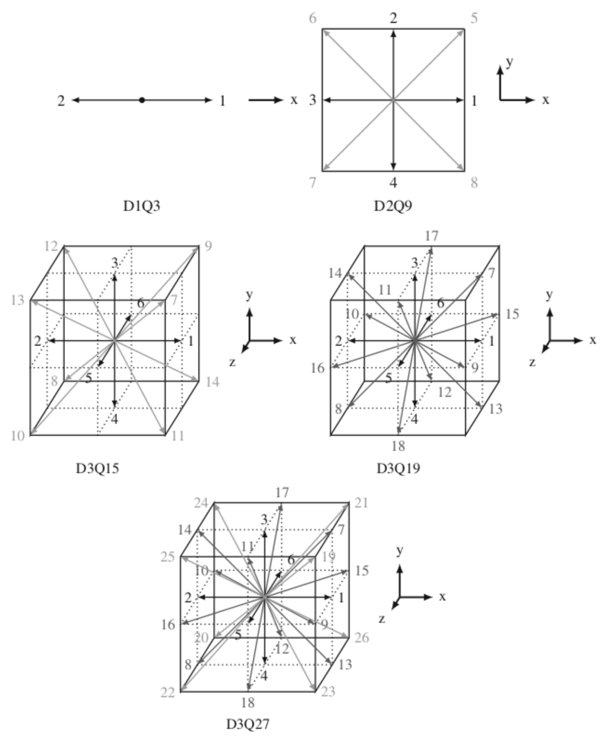
where $f_i\left(\mathbf{x},t\right)$ is the density function representing the probability of finding a particle at position $\mathbf{x}$ and time t with a velocity ${\mathbf{e}}_i$, and $\Delta t$ is the lattice timestep. The right-hand side of the equation contains a collision operator, ${\mathrm{\Omega }}_i$, which can assume different forms. The index i refers to the discrete directions in which the particle can move, which depends on the type of lattice considered for the simulation. Some examples of the most commonly used lattices, such as D2Q9, D3Q19, and D3Q27, are shown in Figure 1, and the choice depends on the characteristics, dimensionality, and symmetries of the problem that one wants to study.

The link between LBM and NS can be found through a multiscale Chapman–Enskog analysis, which involves expressing the populations as a perturbative series centered on the equilibrium density function $f_i^{eq}$,

$$f_i=f_i^{eq}+ϵf_i^{\left(1\right)}+{ϵ}^2{f}_i^{\left(2\right)}+\dots ,$$

(2)

separating the equilibrium from the nonequilibrium part, where $ϵ$ is a smallness parameter. It is possible to show that NS equations are recovered from the solution of Equation (1), and macroscopic quantities such as flow density $\rho$ and velocity $\mathbf{u}$ are recovered as moments of the populations,

$$\begin{array}{cc}\hfill \rho & =\sum _i{f}_i,\hfill \end{array}$$

(3a)

$$\begin{array}{cc}\hfill \rho \mathbf{u}& =\sum _i{f}_i{\mathbf{e}}_i.\hfill \end{array}$$

(3b)

One of the most common and simple forms for the collision operator is

$${\mathrm{\Omega }}_i=-{\displaystyle \frac{f_i-f_i^{eq}}{\tau }},$$

(4)

referred to as the Bhatnagar–Gross–Krook (BGK) operator. It consists of performing the relaxation of the density functions (henceforth called ‘populations’) towards equilibrium, $f^{eq}$; $\tau$ is the relaxation time and is linked to the viscosity of the fluid as

$$\nu =c_s^2\left(\tau -{\displaystyle \frac{1}{2}}\right),$$

(5)

where $c_s$ is called the speed of sound and for most types of lattices is equal to $1/\sqrt{3}$. The equilibrium populations are obtained from

$$f_i^{eq}=w_i\rho \left(1+{\displaystyle \frac{e_{i\alpha }{u}_{\alpha }}{c_s^2}}+{\displaystyle \frac{u_{\alpha }{u}_{\beta }(e_{i\alpha }{e}_{i\beta }-c_s^2{\delta }_{\alpha \beta })}{2c_s^4}}\right),$$

(6)

where $w_i$ are weights specific to the chosen velocity set. Substituting Equation (4) into Equation (1), one obtains the so-called LBGK equation.

The core of the LBM algorithm can be split into two steps, collision and streaming, which are the main reasons behind LBM’s peculiarities. The collision step, corresponding to the right-hand side of Equation (1), is non-linear but local, as it does not require information from neighboring nodes. The opposite can be said about the streaming operation, corresponding to the left-hand side of Equation (1), which is non-local but linear. This is the key property that makes LBM extremely well-suited for high-performance computing on parallel architectures.

The phenomenon to be studied—brine diffusion from outfalls—also deals with the presence of a concentration field, making it necessary to model its presence and evolution. In order to do this, an Advection Diffusion Equation (ADE) must also be solved; due to the similarities between the ADE and the NS equation, it is possible to employ a similar approach to the one described above. The equation to be tackled is

$$\frac{\partial C}{\partial t}+\nabla ·\left(C\mathbf{u}\right)=D{\nabla }^{2}C+q,$$

(7)

where C is a scalar field such as temperature or concentration, q is a source/sink term, which is set to zero in this study, and D is the diffusion coefficient. To solve the ADE with an LBM-based approach, a second set of populations, $\left\{g_i\right\}$, is introduced, which will evolve according to an equation analogous to Equation (1),

$$g_i(\mathbf{x}+{\mathbf{e}}_{\mathbf{i}}\Delta t,t+\Delta t)=g_i(\mathbf{x},t)-{\displaystyle \frac{\Delta t}{{\tau }_g}}\left(g_i-g_i^{eq}\right).$$

(8)

Here, ${\tau }_g$ and $g_i^{eq}$ are the relaxation time and the equilibrium distributions for the set of populations $\left\{g_i\right\}$, respectively. The former is linked to the diffusion coefficient in the ADE via the relation

$$D=c_s^2\left({\tau }_g-{\displaystyle \frac{1}{2}}\right),$$

(9)

while the latter can be expressed as

$$g_i^{eq}=w_{i}C\left(1+{\displaystyle \frac{{\mathbf{e}}_i·\mathbf{u}}{c_s^2}}+{\displaystyle \frac{{\left({\mathbf{e}}_i·\mathbf{u}\right)}^2}{2c_s^4}}-{\displaystyle \frac{\mathbf{u}·\mathbf{u}}{2c_s^2}}\right),$$

(10)

where once again, the speed of sound $c_s$ and the weights $w_i$ depend on the chosen velocity set. The concentration C can be recovered as the zero-th-order moment of the new set of populations,

$$C=\sum _i{g}_i.$$

(11)

As well as the presence of a saline concentration field, the effect of gravity must also be taken into account. In this study, the difference between the jet density ${\rho }_j$ and the ambient fluid density ${\rho }_0$ is assumed to be small, so the Boussinesq approximation is valid, and the density variations can be assumed to affect the flow only via the gravity force term, keeping the incompressibility hypothesis. Thus, the force term considered ${\mathbf{F}}^{ext}$ is equal to

$${\mathbf{F}}^{ext}=-{\rho }_{0}g\left(1+{\displaystyle \frac{{\rho }_s-{\rho }_0}{{\rho }_0}}C\right)\mathbf{k},$$

(12)

where $\mathbf{k}$ is the unit vector aligned with the vertical direction, designated by the Z axis; ${\rho }_s$ is the density of the salt; and $C=C(\mathbf{x},t)$ is the salt concentration at point $\mathbf{x}$ and at time t. There are several possible strategies to add a body force to the simulation; in this work, the one developed by Guo [35] is employed, which relies on adding terms related to the force both in the expression for the velocity Equation (3b) and in the LBGK equation.

Simulations of turbulent flows often require the use of turbulence models to reduce computational costs while retaining essential flow features. In this study, an LES approach integrated into the LBM framework was adopted, following the implementation described by Hou [36]. Specifically, the widely used Smagorinsky subgrid-scale model was employed. It should be noted that this model is known to have limitations in accurately representing turbulence in strongly stratified flows [37,38]. This limitation is particularly relevant for low-Froude number dense jets, where buoyancy and stable density gradients can significantly influence turbulence generation and suppression. Moreover, the Smagorinsky model may introduce excessive eddy viscosity in transitional or low-Reynolds number regimes, potentially dampening the development of resolved turbulence. However, this model was chosen for the present work due to its simplicity and its straightforward implementation in the framework of LBM.

The Smagorinsky model relies on a filtering operation, and the unresolved scales of turbulence are modeled through the introduction of a turbulent viscosity, ${\nu }_t$,

$${\nu }_t={\left(C_S\Delta \right)}^2\sqrt{2S_{\alpha \beta }{S}_{\alpha \beta }},$$

(13)

where $C_S$ is the Smagorinsky constant, which is a numerical quantity typically in the range $0.1\le C_S\le 0.2$, $\Delta$ is the filter width, and $S_{\alpha \beta }$ is the components of the strain rate tensor, which can be obtained through the non-equilibrium populations. In this work, the filter width $\Delta$ is taken equal to the local grid spacing, which is a common practice in LES [39,40]. The total effective viscosity is thus obtained by adding the kinematic and turbulent viscosity ${\nu }_{\mathrm{eff}}=\nu +{\nu }_t$; in turn, the effective relaxation time—which is linked to viscosity—will also be expressed as the sum of two terms, ${\tau }_{\mathrm{eff}}=\tau +{\tau }_t$.

When certain quantities exhibit rapid variations in both time and space, as in the case of turbulent flows, numerical instabilities may arise. In order to mitigate this, a recursive regularization procedure, first presented by [41] and improved by [42], can be applied to the collision operator. At a given iteration, the macroscopic observables—computed in the previous iteration—are used to obtain an approximation of the non-equilibrium part of the population, which is summed to the equilibrium part. Afterwards, the standard BGK operator is applied.

3. Negatively Buoyant Jets in Crossflows

The phenomenon under consideration is that of a vertical saline—and thus, dense—jet of density ${\rho }_j$ released with a velocity $u_j$ from a nozzle of diameter d into a receiving fluid of density ${\rho }_a$$({\rho }_j>{\rho }_a)$, with an ambient crossflow velocity $u_a$. A relevant quantity for describing jet behavior is the densimetric Froude number, defined as

$$F={\displaystyle \frac{u_j}{\sqrt{g_0^{\prime }d}}},$$

(14)

where $g_0^{\prime }=g({\rho }_j-{\rho }_a)/{\rho }_a$ is the initial value of the modified acceleration due to gravity, g. This quantity connects the inertial forces to the buoyancy forces in plumes and is a measure of the importance of the source volume flux.

Because vertical jets fall back directly onto themselves when discharged into a stationary environment, thereby impairing dilution, diffusers are frequently designed with the nozzle inclined at some oblique angle to the horizontal [43]. However, vertical jets do not collapse onto themselves in the presence of even a moderate current and can be more advantageous in specific situations, such as when the current’s direction changes or fluctuates, which is typical of tidal regimes. Gungor and Roberts [44] observed that the dynamical effect of the ambient current is mainly determined by the so-called crossflow parameter,

$$u_{r}F={\displaystyle \frac{u_a}{\sqrt{g_0^{\prime }d}}},$$

(15)

which does not depend on the jet velocity $u_j$.

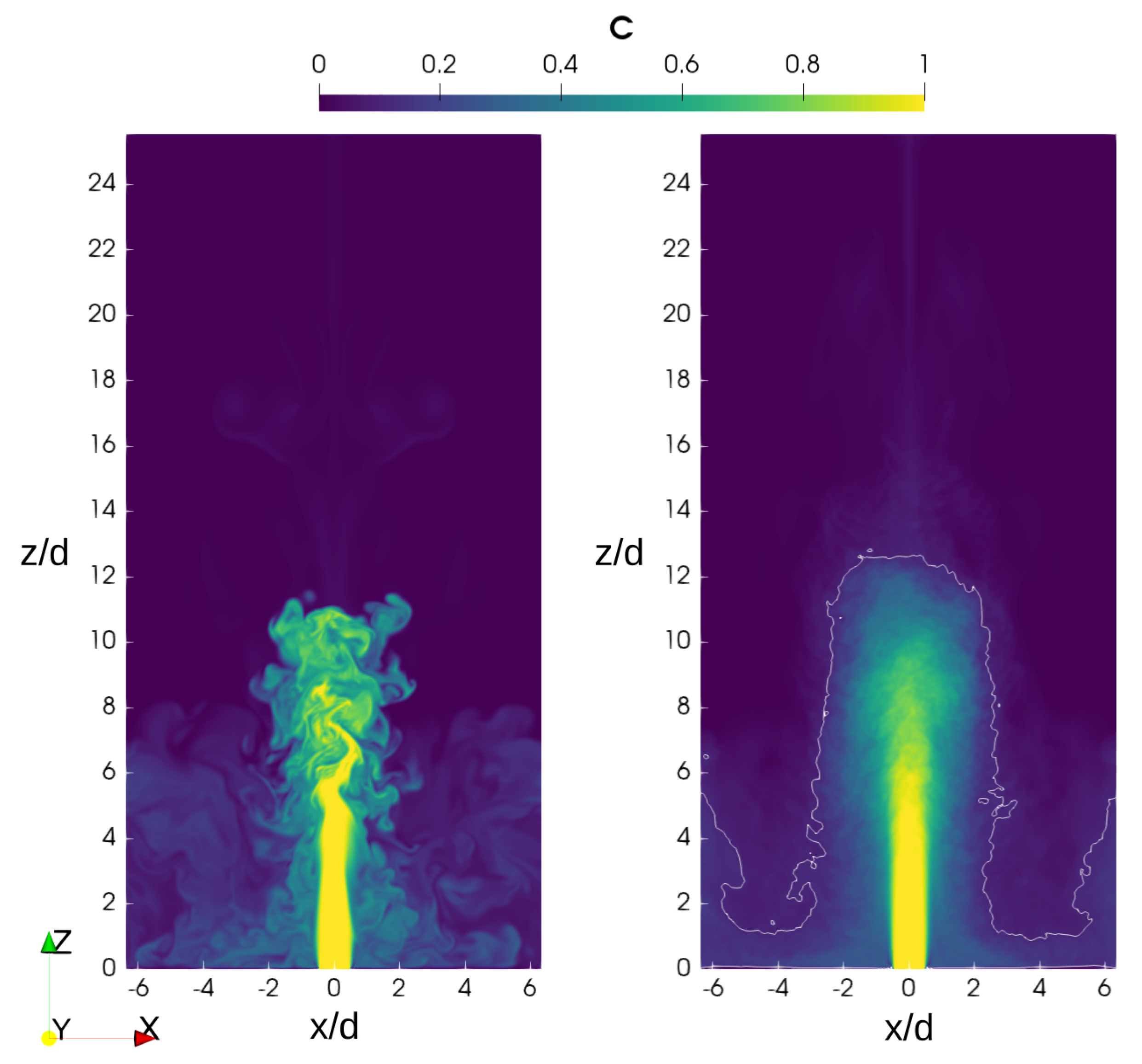
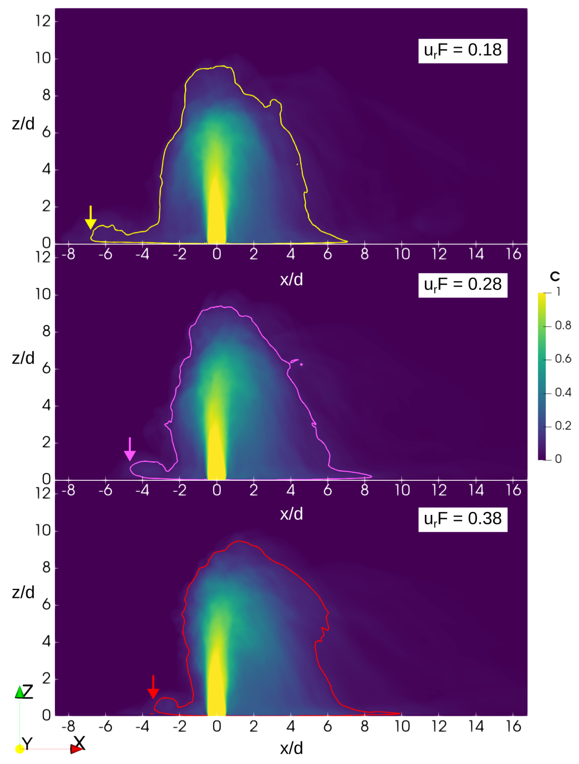
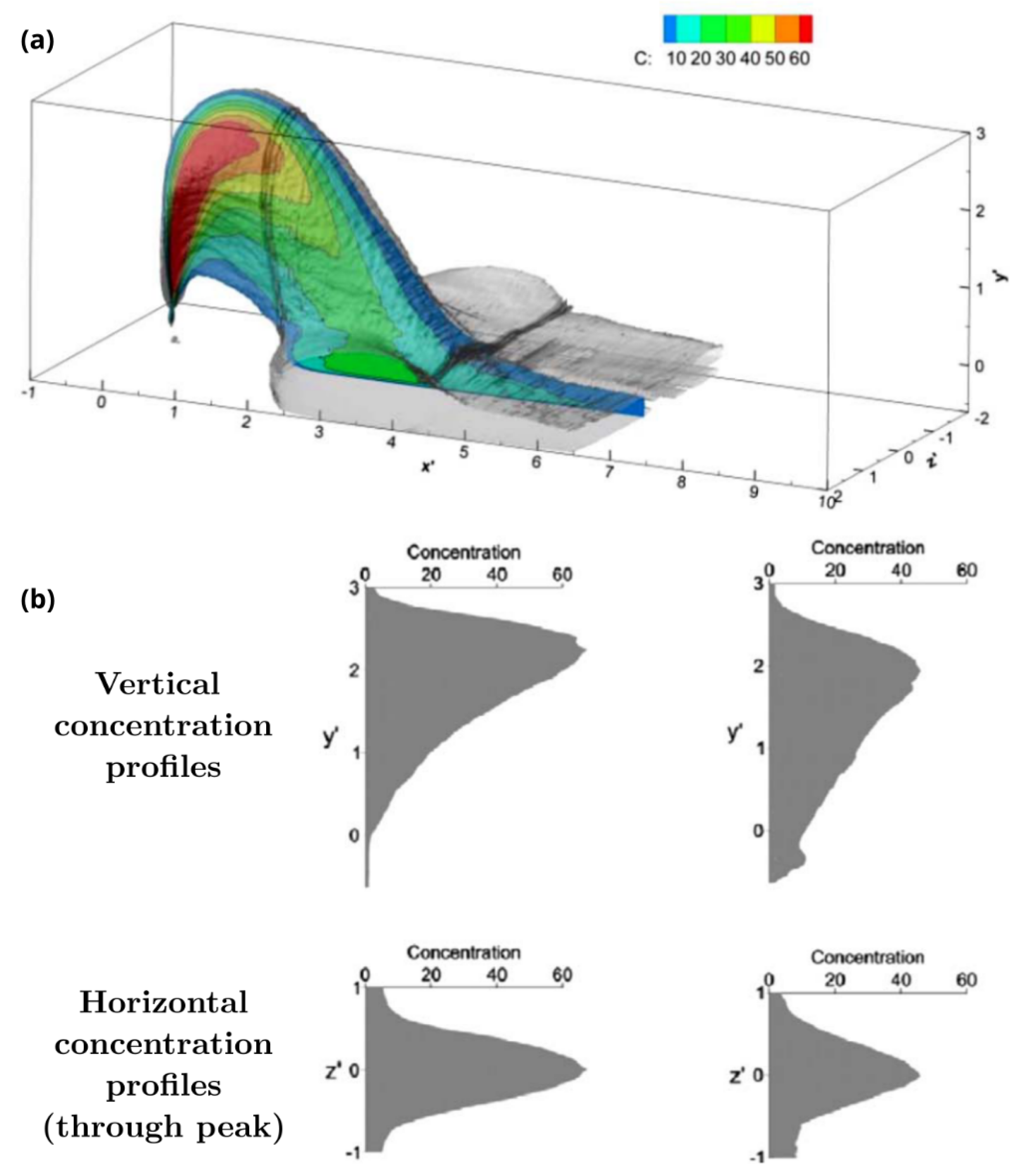
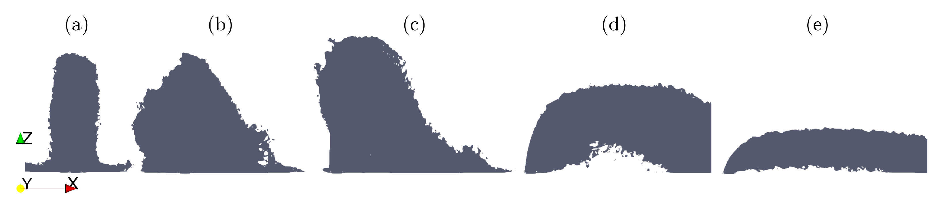
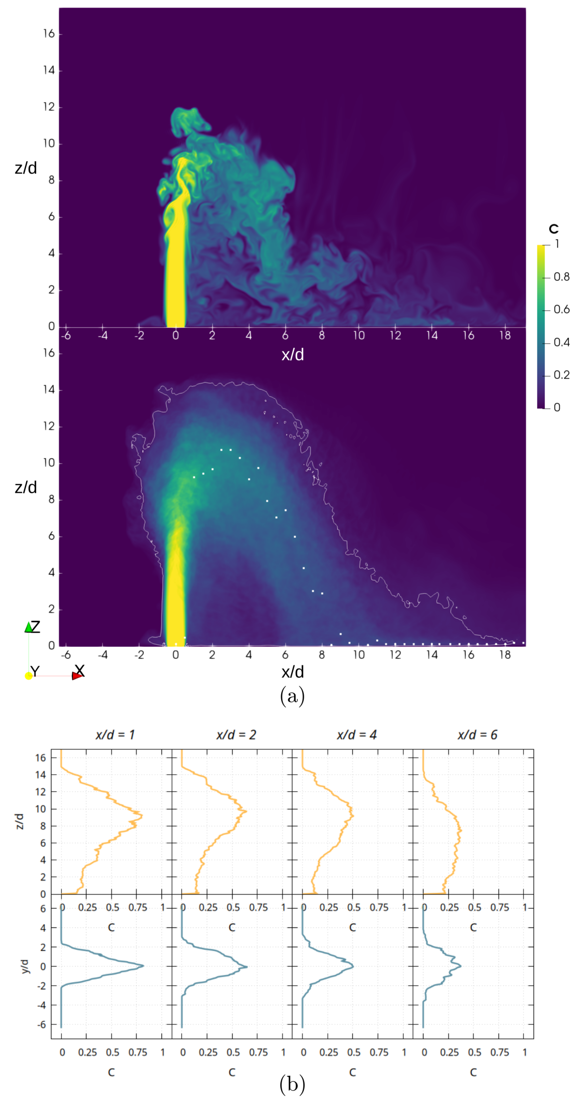
As illustrated in Figure 2, the behavior of the negatively buoyant JICF is strongly dependent on the value of $u_{r}F$. In the absence of a crossflow, the jet falls back on itself, similar to a fountain, and spreads on the bottom as a density current. However, as soon as $u_a>0$, the trajectory of the jet bends in the direction of the ambient flow. It is observed that the jet trajectory reaches a maximum height for values of the crossflow parameter around 0.2 and 0.8, and for $u_{r}F<0.5$, the bottom layer of the jet forms an upstream wedge, whose length decreases as the value of $u_{r}F$ approaches 0.5, as can be inferred from Figure 2 and Figure 3a.

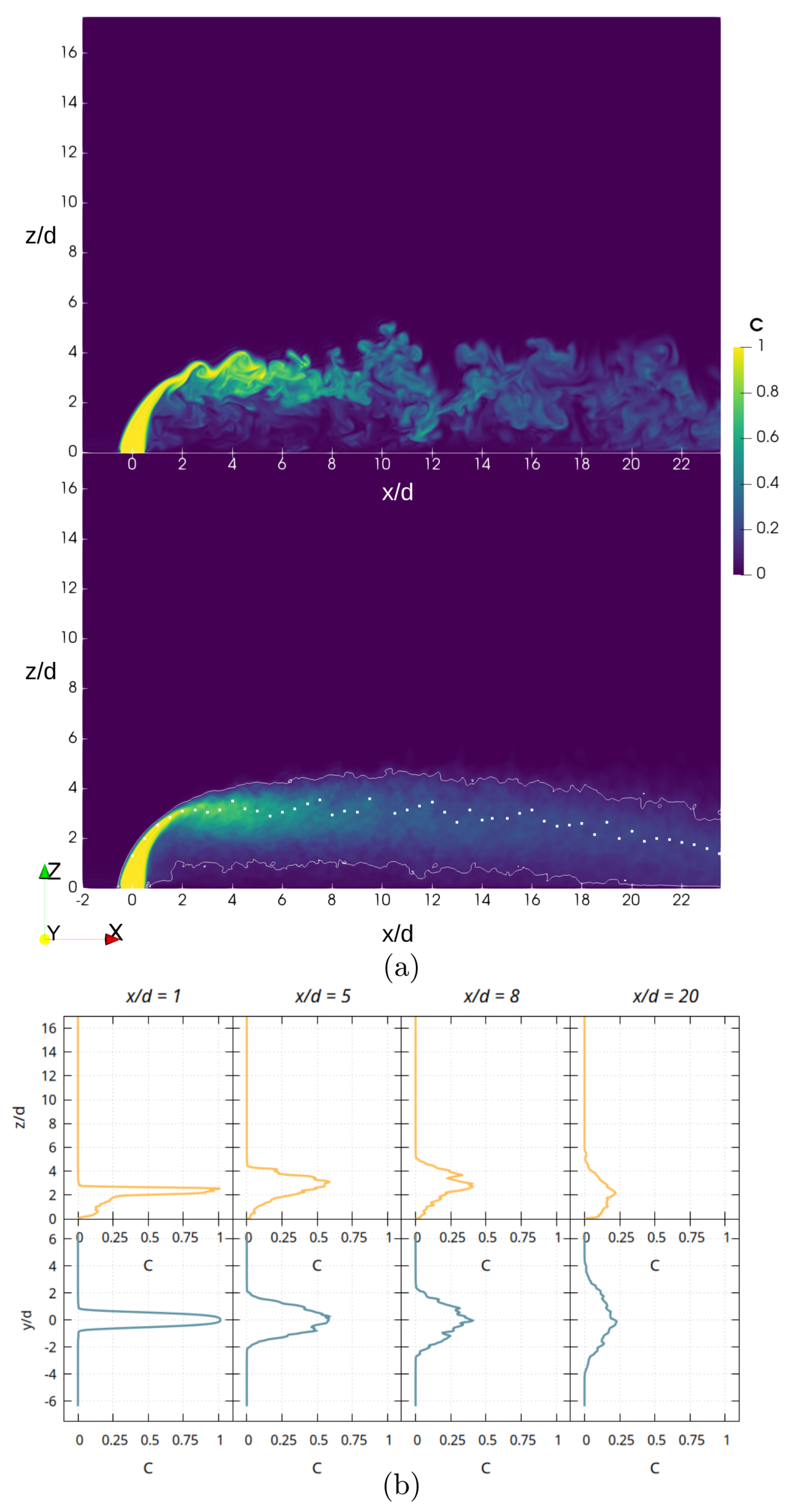
It can be deduced that, for $u_{r}F\ll 1.0$, the current does not significantly affect the jet, which rapidly rises and then falls not very far from the jet nozzle. When $u_{r}F$ becomes approximately equal to 1, this behavior changes, and the descending phase becomes much more gradual while the jet trajectory reaches a lower maximum height. It can be seen from Figure 3b that vertical concentration profiles are especially asymmetrical in the ascending phase due to gravitational instabilities. The horizontal concentration profiles through the peak, on the other hand, are symmetric in both phases. The asymmetry of the vertical concentration profiles will also be less pronounced in the descending phase for jets with $u_{r}F\approx 1.0$ and beyond.

Generally, the jets with a greater ability to diffuse are those with a crossflow parameter $u_{r}F\approx 2.0$. This is due to the fact that, as their trajectory is almost horizontal, they are able to travel across a longer distance before impacting the floor, and they end up being dispersed by ambient turbulence in the receiving waters or being trapped in ambient density stratification, minimizing the impact of the jet fluid on the seabed. This is of particular importance, as the benthic community has limited mobility and is presumably most vulnerable to increased salinity on the sea floor.

Jet trajectories can be defined in a number of ways, and different approaches for their calculation have been followed in the literature. Some are based on velocity maxima [45], while others employ maxima from either the concentration of a passive scalar or from a temperature field [46], sometimes differentiating the two by calling the concentration-based one centerline.

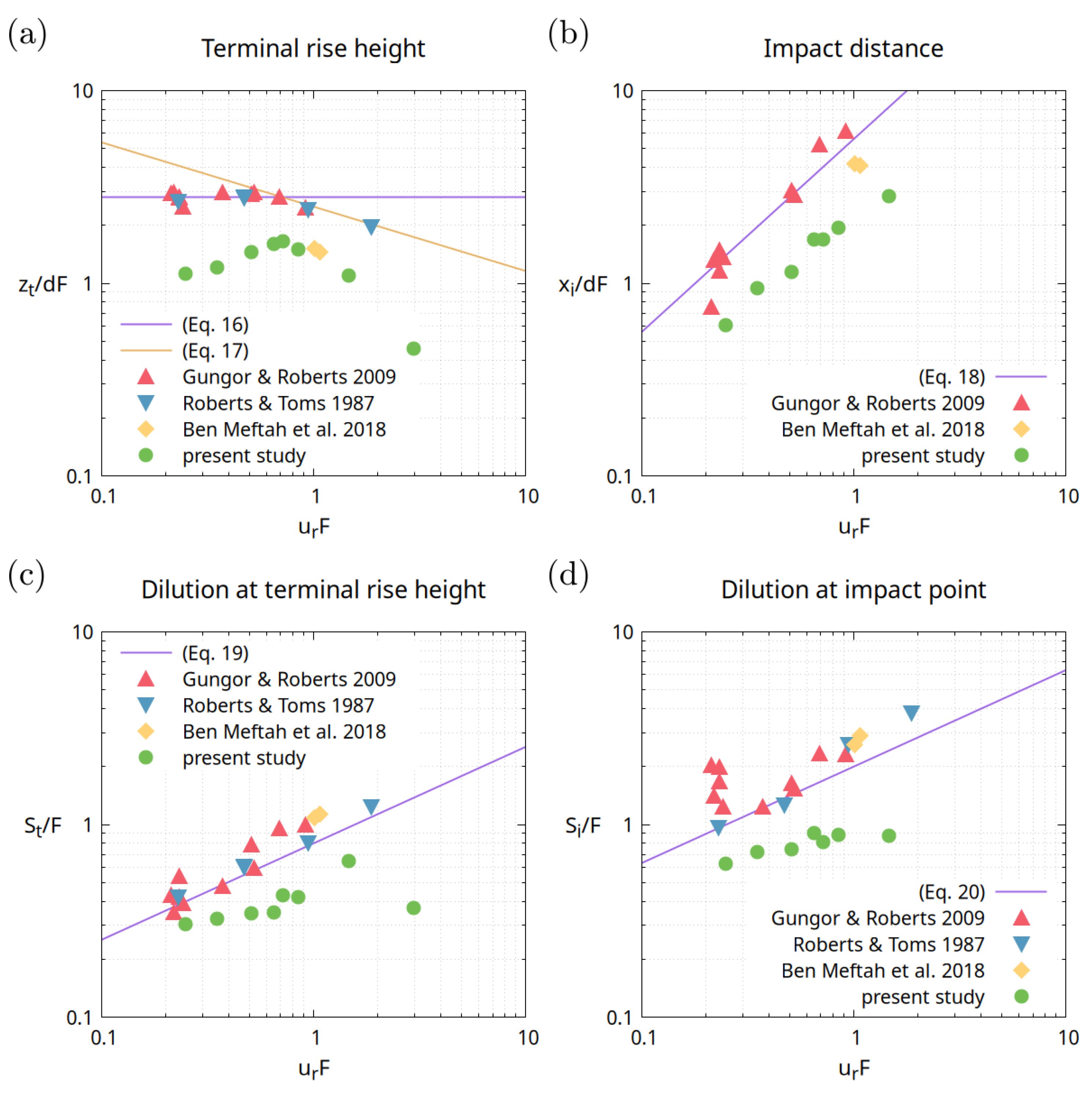
In this work, the jet trajectory of a vertical dense JICF is defined as the curve formed by the locus of maximum saline concentration at the different downstream positions $x/d$, along the axisymmetric plane corresponding to $y/d=0$, following the definition used by Ben Meftah and Mossa [47]. From the jet trajectory, the terminal rise height and impact distance can be extracted. The terminal rise height $z_t/dF$, which is the maximum height the jet reaches along its trajectory, can be expressed with semi-empirical relations derived by Roberts and Toms [48]:

$$\begin{array}{cc}\hfill {\displaystyle \frac{z_t}{dF}}& =2.8\mathrm{for}0.2<u_{r}F<0.8,\hfill \end{array}$$

(16)

$$\begin{array}{cc}\hfill {\displaystyle \frac{z_t}{dF}}& =2.5{\left(u_{r}F\right)}^{-1/3}\mathrm{for}{u}_{r}F>0.8.\hfill \end{array}$$

(17)

From these relations, it is evident that the terminal height reached by a jet is expected to roughly depend solely on its values of $u_{r}F$ and, for jets in a stronger ambient crossflow, F. The impact distance $x_i/dF$ is the downstream distance at which the jet impacts the bottom of the channel, for which Gungor and Roberts [44] derived the relation

$${\displaystyle \frac{x_i}{dF}}=5.6u_{r}F.$$

(18)

Having defined the dilution at a point as $S=(C_0-C_a)/(C-C_a)$, where $C_0$ is the saline concentration at the jet nozzle, and $C_a$ is the ambient saline concentration, Roberts and Toms also introduced semi-empirical power law equations for $S_t/F$, the dilution at the terminal rise height, and $S_i/F$, the dilution at the impact point on the bottom of the channel.

$$\begin{array}{cc}\hfill {\displaystyle \frac{S_t}{F}}& =0.8{\left(u_{r}F\right)}^{1/2},\hfill \end{array}$$

(19)

$$\begin{array}{cc}\hfill {\displaystyle \frac{S_i}{F}}& =2.0{\left(u_{r}F\right)}^{1/2}.\hfill \end{array}$$

(20)

As outlined by Fric and Roshko [49], four fundamental vertical structures are present in a JICF:

• A horseshoe vortex forming upstream of the jet exit;
• Jet shear-layer ring vortices, generated at the windward interface between the jet and the crossflow;
• Unsteady wake vortices beneath the detached jet;
• A counter-rotating vortex pair (CRVP).

All these structures, illustrated in Figure 4, are intertwined as they originate and are affected by the interaction between the crossflow and the jet flow. For a negatively buoyant JICF, it was noted [44,50] that the presence of a CRVP in their flow field emerges in jets whose crossflow parameter is greater than 1.0. This reinforces the statement that negatively buoyant JICF with a higher crossflow parameter tends to have a lower environmental impact, as the CRVP is linked to the mixing of ambient water with the jet fluid in a process called entrainment, where ambient fluid is incorporated in the jet core through “gulps” caused by vortical structures.

4. Numerical Implementation

To conduct the simulations discussed in the following section, a full-LBM-based approach was adopted to solve both the NS equation and the ADE, as described in Section 2. A D3Q27 velocity set (shown in Figure 1) was chosen to solve the hydrodynamics of the system, as it is more appropriate for simulating turbulent flows for isotropy-related reasons, while a D3Q7 lattice was employed for the ADE: it has been shown, in fact, that this type of lattice is sufficient for most diffusion problems [51]. Although anisotropic turbulent diffusion can be relevant in environmental flows, acceptable results can still be obtained by approximating both the diffusion and the eddy viscosity as isotropic [52]. Therefore, this approximation was adopted here for simplicity. As the flows subject to the present study were expected to be turbulent, LES was integrated in the LBM framework, following the procedure detailed above and employing the Smagorinsky model.

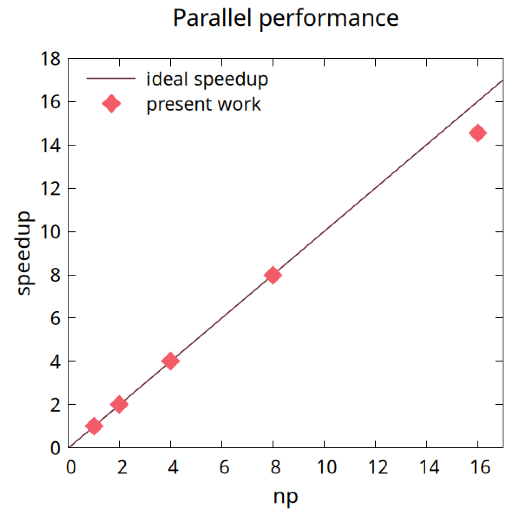
In order to achieve greater numerical stability, the recursive regularization procedure for the collision operator procedure was also carried out. The code employed was developed entirely in-house, in C/C++ language. It was parallel and made use of Message Passing Interface (MPI) libraries for handling communications between different threads. Figure 5 illustrates the speedup (the ratio of the time required to complete a simulation with one MPI process to the time required to complete the same simulation with np MPI processes) of the code for up to $\mathit{np}=16$.

In order to describe the behavior of a vertical dense jet in the presence of an ambient crossflow, the computational domain considered had a cuboid shape to take into account the bending over of the jet in the direction of the crossflow. Specifically, a ratio of 2:1:1 was kept for the length of the system in directions X, Y, and Z, respectively. Unless otherwise specified, the computational grid employed a discretization of 512 points in the streamwise direction (X) and 256 points in the other two directions (Y, Z). The presence of the crossflow was implemented through open boundaries in the streamwise direction X, specifically an inlet where the flow velocity was imposed and an outlet where pressure (density) values were specified. This allowed the flow in the bulk of the domain to be kept at a constant velocity in the absence of the jet. On the floor, which was modeled with a no-slip wall, a round jet inlet was positioned with an imposed uniform velocity profile. The diameter of the nozzle was discretized with 20 grid points and placed at 12.8 diameters downstream of the channel inlet, in the middle of the channel in the Y direction. The top wall was modeled either as a free-slip or as a moving wall with the same velocity imposed in the channel. In the Y direction, periodic boundary conditions were considered, which can be interpreted as a way to model the presence of multiple jets with a spacing equal to the size of the domain in the direction transverse to the ambient flow. A more in-depth description of the boundary conditions employed is given in the following paragraph.

4.1. Boundary Conditions

Boundary nodes in LBM typically require special treatment, as populations streaming inside the domain from boundary nodes are not defined. In this study, the bottom wall of the computational domain was implemented as a simple bounce-back boundary condition based on the idea that populations hitting a rigid wall during propagation are reflected back to where they came from. In order to implement this procedure, one considers that populations leaving the boundary node ${\mathbf{x}}_b$ at time t meet the wall surface at time $t+\Delta t/2$, where they are reflected back with a velocity ${\mathbf{e}}_{\overline{i}}=-{\mathbf{e}}_i$ and arrive at time $t+\Delta t$ back at the node ${\mathbf{x}}_b$ where they came from. For these populations, the streaming step is replaced by

$$f_{\overline{i}}({\mathbf{x}}_b,t+\Delta t)=f_i^{*}(\mathbf{x},t).$$

(21)

While the basic bounce-back principle is used to model stationary walls, the idea behind it can be used to also implement boundary conditions for moving walls. In this case, assuming the wall has a velocity ${\mathbf{u}}_w$, the bounce-back procedure prescribes

$$f_{\overline{i}}({\mathbf{x}}_b,t+\Delta t)=f_i^{*}(\mathbf{x},t)-2w_i{\rho }_w{\displaystyle \frac{{\mathbf{e}}_i·{\mathbf{u}}_w}{c_s^2}},$$

(22)

where ${\rho }_w$ is the density at the wall, which can be extrapolated from the nearest fluid boundary.

Free-slip-type boundaries, which enforce a zero normal fluid velocity $u_n=0$ but place no restrictions on the tangential fluid velocity $u_t$, are implemented with a slight variation on the bounce-back method. Populations leaving a boundary node ${\mathbf{x}}_b$ at time t that meet the free-slip surface at time $t+\Delta t/2$ are reflected specularly, and then they arrive at the node ${\mathbf{x}}_b$ or one of the neighboring ones at time $t+\Delta t$. The standard streaming step for these populations is replaced by

$$f_j\left({\mathbf{x}}_b+{\mathbf{c}}_{j,t}\Delta t,t+\Delta t\right)=f_i^{*}\left({\mathbf{x}}_b,t\right),$$

(23)

where ${\mathbf{c}}_{j,t}={\mathbf{c}}_{i,t}$ is the tangential velocity of the populations, equalling ${\mathbf{c}}_i$ and ${\mathbf{c}}_j$ with their normal velocity set to zero.

The inlet and outlet were obtained as regularized boundary conditions. As the name suggests, they are related to the regularization procedure discussed at the end of Section 2 and specifically to the procedure introduced by Latt and Chopard in [41] and detailed in [53]. It is based on evaluating the non-equilibrium part of the populations based on the knowledge of the populations already known and then reconstructing the missing particle populations in a way that is consistent with the multiscale analysis.

4.2. Domain Size

Given the exploratory nature of this study, aimed at evaluating the potential of the LBM framework to model the behavior of a saline jet in an ambient current, some consideration was made to employ a balanced approach in selecting an appropriate grid size for the simulations presented in the following section.

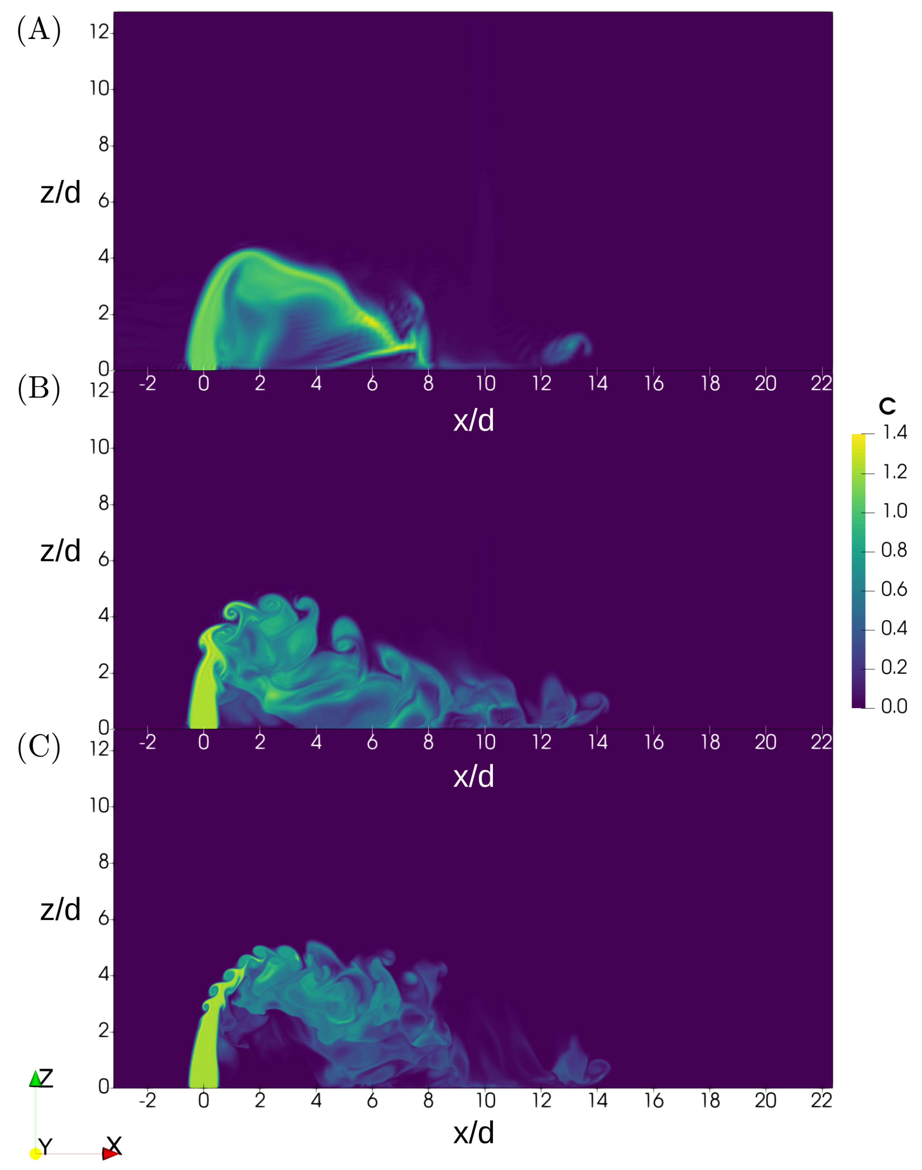
Some tests were performed on a jet with $u_{r}F\approx 1.0$ in order to compare the simulation results of a specific vertical dense JCIF using three differently sized computational domains. Specifically, the behavior of the same vertical dense JICF, with $u_{r}F=1.0$ ($F=4.5$, $Re=3506$, and $u_j/u_a=4.5$), was investigated by running simulations with a domain with a discretization along directions X, Y, and Z, of $256\times 128\times 128$ points (A), $512\times 256\times 256$ points (B), and $1024\times 512\times 512$ points (C). Figure 6 shows the comparison of the instantaneous concentration field in the axisymmetric plane after the same amount of iteration has been carried out in all three cases, each with its own time discretization. Figure 7 compares the streamlines in simulations (A), (B), and (C). It can be seen that for smaller grids, there is a relevant loss of resolution in the vortical structures that appear in the flow, as can be expected. Specifically, the velocity streamlines in simulation (A) highlight that the CRVP is pretty much absent, and the flow in the domain is almost laminar.

Ring vortices are completely absent in this case as well, as can be inferred by both Figure 6 and Figure 7, which also indicate the ability of simulations performed with grid size (B) to correctly describe the formation of vortical structures such as CRVP, ring, and wake vortices, as discussed in more detail in Section 3. The computational domain for simulation (C) seems even more richly populated by turbulent structures, as would be expected from more finely discretized grids.

Despite these differences, the general behavior is consistent throughout the three cases considered. The terminal rise height is roughly the same, and so is the location of the impact with the bottom of the channel, as can be inferred from Figure 6. Due to the jet showing a less turbulent behavior for the lowest resolution grid, the dilution is likely to be underestimated compared with finer grids. Simulation (A) also displays odd values in the concentration map shown in Figure 6: these unphysical values are linked to the insufficient discretization employed, which renders the results inaccurate. Simulations (B) and (C) show better performances in this regard, as the concentration maps relative to these cases display reasonable behavior. In light of this, the medium-sized grid (B) has been deemed to be a reasonable compromise for the scope of this work, as it was still able to capture vortical structures of the JICF with a reduced computational cost.

All the results of the simulations discussed in the following will be presented as dimensionless quantities. Unit conversion between real units and simulation units can be carried out through dimensionless numbers (such as $Re$, $u_r$, F...) and by observing that flows obeying the NS equation are equivalent if they are described by the same dimensionless quantities and the same geometry.

5. Results and Discussion

Several tests were performed on different configurations to observe whether the qualitative behavior of the jet would match the experimental observations made by Gungor and Roberts [44]. Specifically, a set of simulations was carried out, varying the value of the crossflow parameter $u_{r}F$. As discussed in Section 3, the value of this parameter has great importance in enabling the forecast of the potential environmental impact of a jet being released into surface water bodies, as it delineates the descent rate of the vertical jet onto the seabed.

5.1. Jet Behavior

As expected from the discussion in Section 3, the current speed influences the behavior of the jet. Figure 8 shows the time-averaged concentration field in the axisymmetric plane for jets having $u_{r}F=0$ (a), $u_{r}F\approx 0.2$ (b), $u_{r}F\approx 0.5$ (c), $u_{r}F\approx 1.0$ (d), and $u_{r}F\gg 2.0$ (e). The Froude number for these configurations is $F=7.43$, and the jet Reynolds number is $Re\approx 4900$. They are described in detail in the following paragraphs. In Figure 9, Figure 10, Figure 11, Figure 12, Figure 13 and Figure 14, the continuous line contour corresponds to the value of $C=0.08$, which is taken as a reasonable threshold to distinguish between the region of the jet and the ambient flow; moreover, to help visualize the jet, the white dots in Figure 10a, Figure 12a, Figure 13a and Figure 14a mark the trajectory at various distances downstream. The general behavior of the jet at different values of $u_{r}F$ is comparable with the one documented by Gungor and Roberts and illustrated in Figure 2 and will be described in more detail in the following paragraphs.

5.1.1. $u_{r}F=0.0$

If the ambient flow is stagnant, meaning $u_{r}F=0.0$ (corresponding to Figure 8a), the jet undergoes a distinctive behavior: it descends and recoils, creating a flow pattern reminiscent of a fountain (Figure 9). In this scenario, the predominant mixing occurs within the bottom layer of the jet, which spreads radially, similarly to the behavior of a density current, where the fluid moves horizontally due to density differences.

Figure 9. Instantaneous (left) and time-averaged (right) concentration field in the axisymmetric plane ($y/d=0$) for a jet with $u_{r}F=0$. The continuous line contour corresponds to the value of $C=0.08$.

Figure 9. Instantaneous (left) and time-averaged (right) concentration field in the axisymmetric plane ($y/d=0$) for a jet with $u_{r}F=0$. The continuous line contour corresponds to the value of $C=0.08$.

In these conditions, the dilution of the jet is minimal: the dispersal and blending of the jet fluid with the surrounding medium are limited, contributing to a concentrated and less diffused distribution of the passive scalar. It is possible to observe, from Figure 9, that the terminal rise height is around $z_t/d\approx 9.5$, which corresponds roughly to $z_t/\left(dF\right)=2.2$, the expected value for a jet in stagnant water as documented by [54].

5.1.2. $u_{r}F\approx 0.2$

For $u_{r}F\approx 0.2$ (Figure 8b), the trajectory of the jet exhibits a slight deflection, maintaining an almost vertical orientation during its ascent phase and displaying a slightly steeper inclination during descent. Arguably, as can be seen from Figure 10a, there is no distinct separation between these ascent and descent phases, increasing the likelihood of re-entrainment, where the descending flow becomes reintegrated into the ascending flow.

The descent phase begins almost immediately: it can be seen from Figure 10 that the jet has already reached its terminal rise height between 2 and 3 diameters downstream of the nozzle, and it impacts the bottom of the channel around $x/d\approx 4$.

Figure 10. (a) Concentration field in the axisymmetric plane ($y/d=0$) for a jet with $u_{r}F=0.25$ (instantaneous (top) and time-averaged (bottom)). The continuous line contour corresponds to the value of $C=0.08$, while the white dots mark the trajectory at various distances downstream. (b) Vertical concentration profile at $y/d=0$ (orange) and horizontal concentration profiles through the vertical concentration peak (blue) at several distances downstream.

Figure 10. (a) Concentration field in the axisymmetric plane ($y/d=0$) for a jet with $u_{r}F=0.25$ (instantaneous (top) and time-averaged (bottom)). The continuous line contour corresponds to the value of $C=0.08$, while the white dots mark the trajectory at various distances downstream. (b) Vertical concentration profile at $y/d=0$ (orange) and horizontal concentration profiles through the vertical concentration peak (blue) at several distances downstream.

The concentration profiles depicted in Figure 10b conform to the anticipated symmetry in the horizontal profile (taken through the peak in the vertical profile) but display a pronounced asymmetry in the vertical profile, specifically in the descending part of the flow, likely due to the gravitational instability and detrainment. It is interesting to notice the formation of an upstream concentration wedge at the bottom of the channel, the length of which diminishes with the increased strength of the crossflow current, as can be inferred from Figure 11, which shows the length of the wedge for $u_{r}F=0.18$ (top), $u_{r}F=0.28$ (center), and $u_{r}F=0.38$ (bottom). The longest upstream wedge is present for the smallest crossflow parameter, while it tends to disappear the more $u_{r}F$ tends to $0.5$. No CRVP is observed, which is, in fact, expected to appear for higher values of $u_{r}F$.

Figure 11. Upstream wedge formation in jets with $u_{r}F=0.18$ (top), $u_{r}F=0.28$ (middle), and $u_{r}F=0.38$ (bottom) highlighted in the time-averaged concentration field in the axisymmetric plane ($y/d=0$). The continuous line contour corresponds to the value of $C=0.08$.

Figure 11. Upstream wedge formation in jets with $u_{r}F=0.18$ (top), $u_{r}F=0.28$ (middle), and $u_{r}F=0.38$ (bottom) highlighted in the time-averaged concentration field in the axisymmetric plane ($y/d=0$). The continuous line contour corresponds to the value of $C=0.08$.

5.1.3. $u_{r}F\approx 0.5$

When the current speed is increased to $u_{r}F\approx 0.5$, the upstream wedge disappears and is completely absent for $u_{r}F\approx 0.6$ (Figure 12a). As for the case where $u_{r}F\approx 0.2$, the ascending part of the jet is almost vertical, but the descending phase is more gradual here. In light of the definition of the trajectory introduced above, and by comparing Figure 10b and Figure 12b, it can be observed that the impact point of the jet with the bottom of the channel is farther downstream compared with the case where $u_{r}F\approx 0.2$, and it is at around 8 diameters from the jet nozzle.

Similarly to what happens for $u_{r}F\approx 0.2$, the vertical concentration profile in the descending phase displays a strong asymmetry, and the horizontal profile taken through the peak is more symmetrical (Figure 12b). Also, in this case, the detrained flow can be entrained back in the rising jet, and the internal mixing due to the gravitational instability can affect peak concentration, impacting the shapes of the mean concentration profiles. The formation of a CRVP is not observed.

Figure 12. (a) Concentration field in the axisymmetric plane ($y/d=0$) for a jet with $u_{r}F=0.51$ (instantaneous (top) and time-averaged (bottom)). The continuous line contour corresponds to the value of $C=0.08$, while the white dots mark the trajectory at various distances downstream. (b) Vertical concentration profile at $y/d=0$ (orange) and horizontal concentration profiles through the vertical concentration peak (blue) at several distances downstream.

Figure 12. (a) Concentration field in the axisymmetric plane ($y/d=0$) for a jet with $u_{r}F=0.51$ (instantaneous (top) and time-averaged (bottom)). The continuous line contour corresponds to the value of $C=0.08$, while the white dots mark the trajectory at various distances downstream. (b) Vertical concentration profile at $y/d=0$ (orange) and horizontal concentration profiles through the vertical concentration peak (blue) at several distances downstream.

5.1.4. $u_{r}F\approx 1.0$

When $u_{r}F\approx 1.0$, the behavior of the jet begins to show different characteristics (Figure 13). The trajectory of the jet displays a substantial bending, as shown in Figure 13a; the jet impacts the channel bottom at a position significantly downstream of the nozzle, towards the end of the computational domain. The ascent and descent phases are clearly separated, and, unlike the previously analyzed cases, the terminal rise height achieved is significantly lower, which is to be expected, as discussed in Section 3.

By looking at the time-averaged concentration profiles in Figure 13b, it is possible to see that the asymmetry is still very present in the ascending phase in the vertical profile. The descent phase for a jet with $u_{r}F\approx 1.0$ is expected to be characterized by vertical concentration profiles where the asymmetry is less pronounced, as observed around $x/d=8$ in Figure 13b. This is, however, not very clearly captured, probably due to a too-low terminal rise height of the jet, which does not allow it to descend for long enough for the profile to actually become fully symmetrical. In this flow regime, the jet distinctly exhibits its characteristic counter-rotating vortex pair, as will be detailed in Section 5.3.

Figure 13. (a) Concentration field in the axisymmetric plane ($y/d=0$) for a jet with $u_{r}F=1.46$ (instantaneous (top) and time-averaged (bottom)). The continuous line contour corresponds to the value of $C=0.08$, while the white dots mark the trajectory at various distances downstream. (b) Vertical concentration profile at $y/d=0$ (orange) and horizontal concentration profiles through the vertical concentration peak (blue) at several distances downstream.

Figure 13. (a) Concentration field in the axisymmetric plane ($y/d=0$) for a jet with $u_{r}F=1.46$ (instantaneous (top) and time-averaged (bottom)). The continuous line contour corresponds to the value of $C=0.08$, while the white dots mark the trajectory at various distances downstream. (b) Vertical concentration profile at $y/d=0$ (orange) and horizontal concentration profiles through the vertical concentration peak (blue) at several distances downstream.

5.1.5. $u_{r}F\approx 2.0$

If the crossflow is even more intense, for $u_{r}F\approx 2.0$ and beyond, the trajectory of the jet exhibits a substantial bending, becoming almost horizontal (Figure 14a). In fact, as already discussed, jets with higher values of the crossflow parameter tend to be dispersed by ambient turbulence more efficiently, as they do not immediately fall back on the floor.

Figure 14. (a) Concentration field in the axisymmetric plane ($y/d=0$) for a jet with $u_{r}F=2.97$ (instantaneous (top) and time-averaged (bottom)). The continuous line contour corresponds to the value of $C=0.08$, while the white dots mark the trajectory at various distances downstream. (b) Vertical concentration profile at $y/d=0$ (orange) and horizontal concentration profiles through the vertical concentration peak (blue) at several distances downstream.

Figure 14. (a) Concentration field in the axisymmetric plane ($y/d=0$) for a jet with $u_{r}F=2.97$ (instantaneous (top) and time-averaged (bottom)). The continuous line contour corresponds to the value of $C=0.08$, while the white dots mark the trajectory at various distances downstream. (b) Vertical concentration profile at $y/d=0$ (orange) and horizontal concentration profiles through the vertical concentration peak (blue) at several distances downstream.

The descent phase is even more gradual than in the case of $u_{r}F\approx 1.0$, with similar vortical structures. Here, as well, the vertical concentration profiles in the descending phase are supposed to be less asymmetric than the ones in the ascending phase (Figure 14b), although this is not clearly visible due to the proximity to the bottom and the horizontal concentration profile through the peak is symmetrical.

The characteristics of simulated negatively buoyant JICF pertaining to several typical values of the crossflow parameter $u_{r}F$ described above match to a good degree the expectations from literature, as well as the behavior of vertical and horizontal concentration profiles. As detailed in Section 3, in fact, the current speed greatly influences the behavior of the jet. Higher values of $u_{r}F$ were associated with an increased capacity of the jet to travel further downstream and thus to entrain more ambient fluid before impacting the floor. The general behavior of the jet at different values of $u_{r}F$ is comparable with the one documented by Gungor and Roberts and illustrated in Figure 2.

5.2. Terminal Rise Height, Impact Distance, Dilution

In addition to the qualitative observations on the general behavior of vertical dense jets in the presence of an ambient crossflow with varying intensity, detailed in the previous sections, a comparison with experimental measurements and semi-empirical relations was carried out. Specifically, terminal rise height, impact distance, dilution at terminal rise height, and dilution at impact point were extracted from simulated jets corresponding to different values of the crossflow parameter $u_{r}F$. The results are presented in

Table 1. Values of $z_t/dF$, $x_i/dF$, $S_t/F$, and $S_i/F$ obtained for vertical dense JICF with $F=7.43$ with varying values of the crossflow parameter.

${\mathit{u}}_{\mathit{r}}\mathit{F}$	${\mathit{z}}_{\mathit{t}}/\mathit{dF}$	${\mathit{x}}_{\mathit{i}}/\mathit{dF}$	${\mathit{S}}_{\mathit{t}}/\mathit{F}$	${\mathit{S}}_{\mathit{i}}/\mathit{F}$
0.25	1.13	0.61	0.30	0.63
0.35	1.21	0.94	0.32	0.72
0.51	1.45	1.14	0.35	0.75
0.65	1.61	1.68	0.35	0.90
0.72	1.65	1.68	0.43	0.81
0.85	1.50	1.94	0.42	0.89
1.46	1.10	2.83	0.65	0.87
2.97	0.48	-	0.37	-

and plotted in Figure 15 along with experimental results from Gungor and Roberts [44], Roberts and Toms [48], and Ben Meftah et al. [47,50], and semi-empirical relations, i.e., Equations (16)–(20). Values of the impact distance and of the dilution at the impact point are not indicated for the jet with $u_{r}F=2.97$, as jets with higher crossflow parameters tend to have more gradual descent phases and not impact the bottom of the channel before the end of the computational domain.

The results concerning the terminal rise height are presented in Figure 15a. A discrepancy of approximately a factor of two is observed, with the exception of the two jets reported by Ben Meftah et al. [47,50], which exhibit Froude numbers of 7.7 and 9.8—values that are more comparable to those characterizing the jets analyzed in the present study. Nevertheless, the overall trend remains consistent, with higher terminal rise heights observed under weaker ambient flow conditions ( $0.2<u_{r}F<0.8$). In particular, there is a strong agreement in the transition from $u_{r}F<0.8$ to $u_{r}F>0.8$, which is clearly captured by the numerical simulations carried out in the present study.

The analysis of the jet impact distance reveals that the values obtained in the present study are lower than those reported in the literature, as illustrated in Figure 15b. This deviation is nonetheless consistent with the observed terminal rise heights, as a reduced maximum elevation causes the jet to descend and touch the bottom at a more upstream location.

Figure 15c demonstrates good agreement with the trend reported in the literature for dilution at the terminal rise height, although the absolute values obtained in the present study remain lower. This discrepancy is consistent with the reduced terminal heights observed, which lead to a more compact jet structure. As a result, the saline concentration is advected over a shorter trajectory and entrains a smaller volume of ambient fluid. The jet corresponding to $u_{r}F=2.97$ exhibits the largest deviation from the expected results. This can be attributed to the fact that, in this case, the peak rise height occurs significantly further downstream, where the jet has undergone substantial lateral spreading. Additionally, the use of periodic boundary conditions in the transverse direction allows saline concentrations to re-enter the domain from the sides, thereby artificially reducing the dilution values.

Upon impingement on the channel bottom, the jet begins to spread laterally, and due to the periodicity in the transverse direction, the recirculation of jet fluid within the domain leads to an artificial increase in concentration over time, influencing the dilution at the impact point, shown in Figure 15d.

Overall, the simulated jets in the present work systematically underestimate the four quantities, although the key trends are generally well captured. The reason behind this result could be attributed, at least in part, to the limitations of the Smagorinsky subgrid-scale model. Specifically, its tendency to overpredict eddy viscosity in transitional and low-Reynolds number regimes can lead to excessive damping of turbulence, thereby reducing vertical momentum transfer and entrainment essential for jet rise against the crossflow. In addition, physical considerations may contribute to the discrepancies between the results presented in this work and the experimental results in the literature. Indeed, the majority of experimental studies investigating the behavior of negatively buoyant JICF—including those used to derive the semi-empirical relations presented in Equations (16)–(20)—have been conducted for Froude numbers greater than 20 [44,48]. Such conditions minimize the influence of the source volume flux and result in jets with higher-reaching trajectories, thereby facilitating experimental measurements. However, to maintain a manageable computational domain size and consider the connection between the Froude number and the maximum height reached by the jet, the tests presented in this study were carried out with Froude numbers ranging from 2.5 to approximately 10. The results shown in Figure 15 are characterized by $F=7.43$.

5.3. Vortical Structures

It is insightful to investigate the ability of the numerical model to capture the various vortical structures that are typical of buoyant jets in crossflows. A useful way to visualize vortical structures in computational domains is to make use of a quantity called the Q-criterion, which is defined as $\tilde{Q}=\left({\parallel \mathrm{\Omega }\parallel }^2-{\parallel S\parallel }^2\right)/2$, where S and $\mathrm{\Omega }$ are, respectively, the symmetric and antisymmetric parts of the velocity gradient tensor $\nabla \mathbf{u}$. S is the strain rate tensor and areas where the magnitude of $\mathrm{\Omega }$ is larger than the strain rate magnitude (i.e., $\tilde{Q}>0$) correspond to locations of vortices.

The presence of a CRVP for jets with $u_{r}F>1.0$ has been mentioned in Section 3, and it can be inferred by looking at streamlines and vortical structures, as shown in Figure 16 and Figure 17 for jets with $u_{r}F\approx 1.0$ and $u_{r}F\approx 2.0$, respectively. In these two figures, the formation of a CRVP is illustrated, showing its evolution through Q-criterion isocontours (on the left), around which streamlines wrap to indicate the flow direction (in the middle) and the effect of the vortex pair on the instantaneous concentration field (on the right).

The CRVP’s presence can also be inferred by looking at velocity profiles on planes perpendicular to the jet trajectory, where the typical kidney shape can be seen in the inset of Figure 18. From Figure 18, it is also possible to recognize the presence of ring vortices on the leading edge at the boundary between the jet and the ambient flow and wake vortices underneath the jet. Their presence is especially evident on larger grids, as was seen in Figure 7.

Out of the four fundamental vortical structures presented in Section 3, only three were successfully represented. The presence of the CRVP in jets with $u_{r}F>1.0$ indicates a more complex flow structure, introducing rotational elements that influence the trajectory and behavior of the jet as it interacts with the surrounding environment and enhances dilution. Wake vortices underneath the jet were present but very localized, which was possibly linked to the small Froude number F of these simulations, which also results in the jet’s terminal rise height being relatively lower and the jet not leaving enough space underneath to allow for a proper wake development. Ring vortices were visible on the leading edge of the jet. There was, however, no evidence of a horseshoe vortex upstream of the jet nozzle. This could be due to insufficient discretization, especially near the wall in the vertical direction, not allowing this type of vortex to be resolved.

6. Conclusions

This work detailed the simulation efforts using an in-house code based on a full-LBM approach to explore the evolution of vertical dense jets, including their vertical and horizontal concentration profiles, the formation of vortical structures, and the measurement of relevant quantities such as terminal rise height, impact distance, dilution at terminal rise height, and dilution at impact point. These simulations showed a promising level of agreement in terms of expected qualitative behavior derived from experimental observations. The numerical results for relevant quantities were systematically underestimated, although the key trends were correctly identified, and the formation of three of the four fundamental vortical structures of JICF was successfully captured, with the exception of the horseshoe vortex. The results indicate a good foundation for using the LBM approach in capturing the complex dynamics of JICF. In a post-exascale world, where supercomputers are able to perform near or above ${10}^{18}$ floating point operations per second, algorithm scalability is a fundamental asset. Because of this, LBM’s role in HPC applications is becoming more and more prominent. In this context, the findings of this preliminary work confirm it would be worthwhile to further investigate this method’s applicability as a tool to assess the environmental impact of wastewater diffusion in surface water bodies.

The next fundamental steps to improve LBM simulations of vertical dense JICF include implementing mesh refinement strategies, which would enable simulating larger computational domains at reasonable computational cost while allowing for finer grids close to the jet inlet. In addition, employing dynamic subgrid-scale models such as the ones proposed by Germano and Lilly [55,56] may mitigate the limitations of Smagorinsky for transitional or low-Reynolds number regimes. Finally, including a turbulent inflow for the jet inlet might improve jet entrainment and structure, leading to more accurate predictions of dilution. Going forward, it would be valuable to conduct a more extensive comparison between numerical results and experimental data, considering vertical and horizontal profiles of velocity and concentration and turbulent quantities, to assess the accuracy of the simulations and further consolidate LBM as a reliable and robust tool for studying brine outfall dispersion.