Development of an Anisotropic Porous Model of a Single Cow for Numerical Barn Simulations—A Numerical Study

Abstract

Computational fluid dynamics (CFD) can be used to analyze the airflow patterns within a naturally ventilated cattle barn in detail, taking into account the influence of the animals. Typically, animals are modelled either as solid obstacles or as a porous block representing the entire animal-occupied zone (AOZ). In the latter approach, extensive pre-simulations are required to determine the appropriate resistance parameters. This study developed a cow model that captures the general influence of the animals, is easy to implement without the need for extensive pre-simulations, and can be applied to various barn types and herd sizes. It is based on a porous block for a single animal. The anisotropic parameters for pressure drop and heat flux were derived from a simplified 3D cow model under different wind speeds, flow directions, cow positions, and ambient temperatures. These parameters were then incorporated into the newly developed porous cow model using regression curves. A comparison between the solid and porous modelling approaches in a randomly selected AOZ showed good agreement in terms of pressure drop and downstream temperature distribution.

1. Introduction

To understand the emission behaviour of a naturally ventilated dairy barn, it is necessary to know the airflow pattern inside the barn. This has a significant influence on the volume flow rate that goes through the barn and transports the volatile emissions. However, measuring these quantities is very difficult due to the large openings in the side walls [1]. In addition, the flow through the barn is directly influenced by the animals themselves due to their spatial extension and the heat they produce [2].

In recent years, computational fluid dynamics (CFD) has become a very popular tool to support measurements of naturally ventilated dairy barns [2,3,4,5]. This allows the spatial resolution inside the building to be implemented with almost infinite accuracy. Animals can also be modelled. However, modelling them directly would result in a large number of elements, leading to long simulation times and more difficult convergence [2,6]. One approach to reduce the elements and complexity is to model the animal-occupied zones (AOZs) as blocks of porous media, which has proven to be a good compromise between accuracy, computational and modelling time, and results [6,7,8,9].

The authors of [2] were, to the authors’ knowledge, the first to model the coefficients of the AOZ as anisotropic. They found regression curves for the resistance coefficients responsible for the pressure drop, but also for the heat flux coefficients. This allowed them to implement the behaviour of these quantities as a function of different wind speeds and directions. The results were in good agreement with the fully modelled approach.

However, some work needs to be carried out in advance in order to model a complete AOZ as a porous block. For each AOZ, all the necessary parameters for each specific case (i.e., number of animals in the AOZ, flow velocity, outside temperature, and geometric size of the AOZ) must be found before the actual simulation of the barn is carried out [9]. This takes a lot of time and effort and makes it difficult to have case studies for whole barns or comparisons between different barns within a project.

To overcome this, the authors of the present study developed a new approach to model the AOZ. Instead of modelling an entire AOZ as a porous medium, the approach here is to model an individual cow as a porous block and combine these individual cows into the herd within the barn for the final simulation. This eliminates the need to run AOZ-defining simulations in advance once the single-cow model is ready for use. It will only be necessary to implement the porous cow model in the simulation and place the blocks at the cow positions before running simulations with different boundary conditions. The following steps were taken to develop this model:

• Find anisotropic parameters for the pressure drop and heat transfer for a single cow modelled as a porous block as a function of wind speed, cow position, wind direction, and ambient temperature.
• Implement these parameters into the porous media model via regression curves.
• Validate the porous model approach with a random AOZ to compare with modelling using simplified solid cow geometries.

2. Materials and Methods

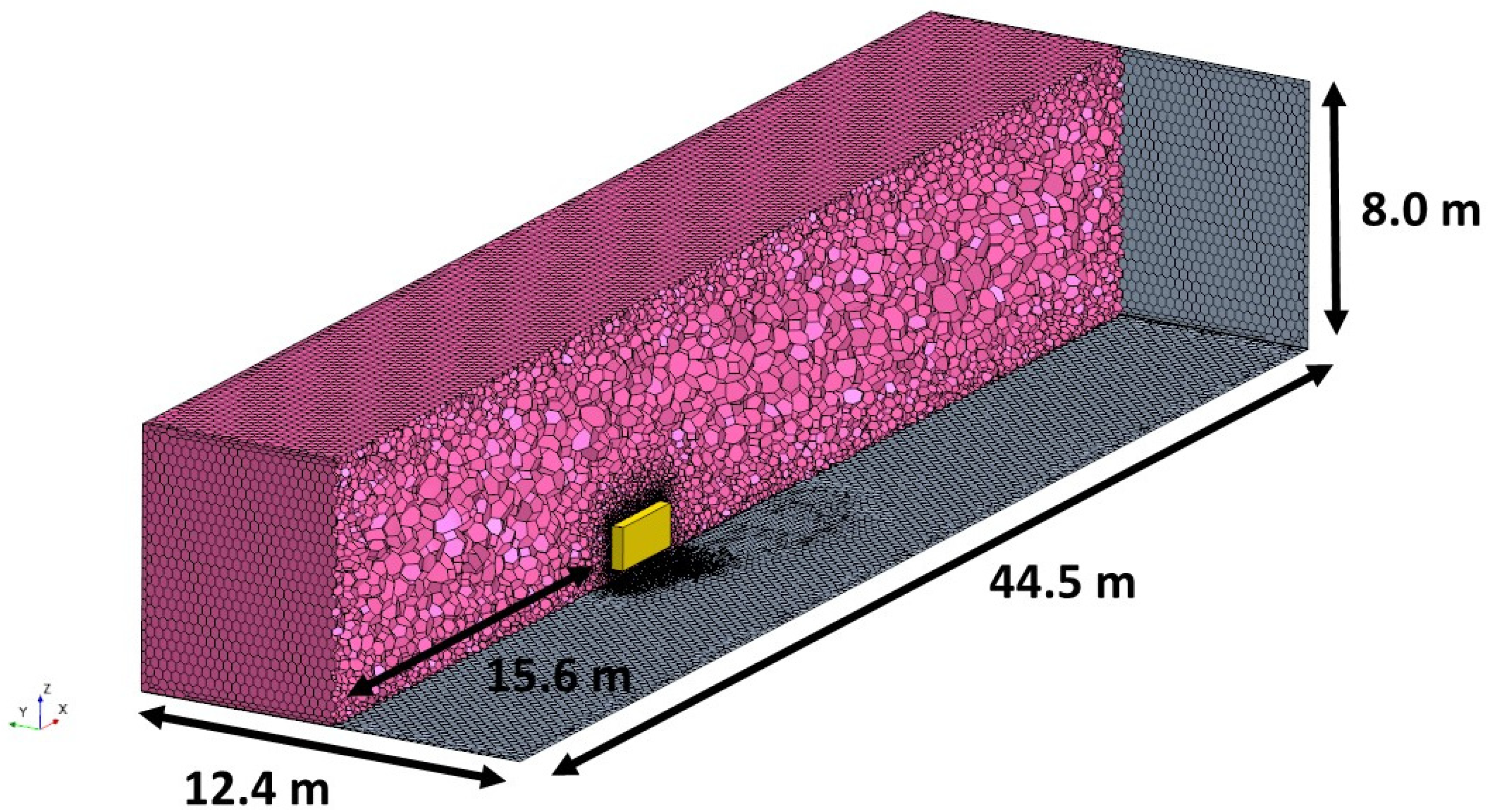
2.1. General Settings for the Simulations

The three-dimensional Reynolds-Averaged Navier–Stokes (RANS) equations were calculated using the commercial software Star-CCM+ in version 15.06.008. Turbulence was modelled using the K-Omega SST model when using a solid model approach. It has advantages over the standard K-Epsilon model in terms of velocity and temperature measurements [10]. This is especially important when evaluating the heat flux of the solid cows to determine the accompanying parameters. With a fine mesh resolution, it is advised to use the K-Omega SST model here [11,12,13]. Using the porous model approach when comparing different AOZs, the turbulence was modelled with the realizable K-Epsilon model for reasons of reaching a better overall convergence. Furthermore, regarding the pressure drop of an AOZ, this turbulence model might be superior to the K-Omega SST model [14]. Meshing was carried out in Star-CCM+. Details of the meshes used are given in the sections below. Time independence (steady state) and a coupled manner of pressure and velocity were further settings for the simulations. A constant density combined with the Boussinesq approximation was chosen to account for buoyancy effects. This is suitable for cases where there is no significant difference between the ambient temperature and the temperature of the heat exchanger [2]. The inlets were modelled as velocity inlets, and the outlets were modelled as pressure outlets with an outlet pressure of 0 Pa. The walls were no-slip walls. Convergence was considered achieved when the global normalized residuals were below 10⁻³ and below 10⁻² for the energy of cows and NH₃, together with no significant change in the monitored coefficients of interest (pressure drop, heat transfer, surface-averaged temperature, and volume flow rate).

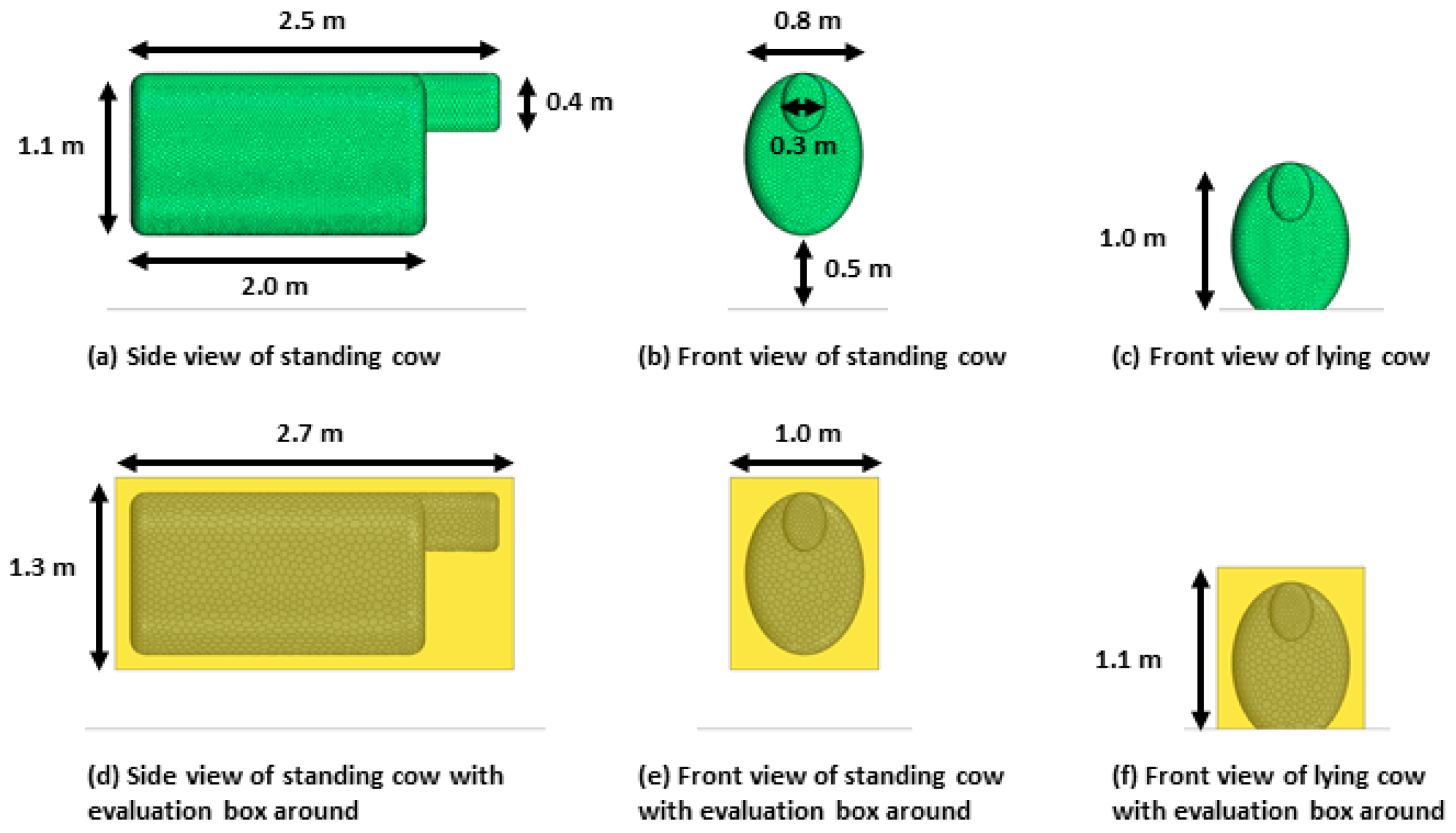
2.2. The Solid and Porous Cow Model

For the solid cow, the authors used a simplified model of the one presented by [7]. It consists of a combination of two differently sized cylinders. Figure 1a–c show its dimensions. Mondaca and Choi [15] showed that the accuracy of the simplified cow model in terms of simulating pressure drop and heat transfer is almost as good as a detailed solid model. Since many simulations have to be performed to find the resistance parameters, the use of the simplified model saves time as it requires fewer elements than the detailed cow model. Following the reasoning of [13], the legs of the standing cow were omitted because the main influence of the individual cow on the flow is considered to come from the body. For the lying cow, the standing cow model was translated by 0.60 m in the negative z-direction. The pressure drop and heat transfer parameters were determined for those two positions. The surface area A in m² exposed to the airflow is 7.6 m² for the standing cow and 6.6 m² for the lying cow.

To evaluate the pressure drop, a box was constructed around the solid cow shown in Figure 1d–f. The sides of the box have a distance of 0.1 m from the outer edges of the cow. They are modelled as internal interfaces so that they do not affect the flow but can act as evaluation planes. This box will later be used for the porous cow model.

The solid cow was used in the simulations to determine the pressure drop and heat dissipation of the single cow. The surface was meshed with polyhedral cells and a target surface size of 0.06 m. Refinements at the edges of the cylinders with a target surface size of 0.025–0.040 m ensured convergence of the solution. To model the porous cow, the block was meshed with polyhedral cells and a target surface size of 0.075–0.125 m.

2.3. Porous Media Modelling

The general approach to finding the coefficients for the pressure drop and heat transfer of the porous model is similar to that of Doumbia et al. [2], but in this case, it is only for a single cow.

Simcenter Star-CCM+ provides two approaches to modelling a porous medium: the superficial velocity formulation and the physical velocity formulation. The former uses a theoretical velocity that takes into account the velocity change due to the area change caused by the porosity. The latter calculates the velocity directly. For the physical velocity formulation, there are two ways of simulating heat transfer. One uses thermal equilibrium between the solid and fluid phases, and the other allows different temperatures of the fluid and solid phases to be taken into account.

The superficial velocity formulation was used to find the resistance coefficients for a given pressure drop. To find the heat transfer coefficients, the authors used the physical velocity formulation with the non-equilibrium state to capture the difference between the air and cow temperatures.

2.3.1. Pressure Drop

Two resistance coefficients are required to model the pressure drop in a porous region: P_v and P_i for the viscous (linear) and inertial (quadratic) resistances, respectively. Simcenter Star-CCM+ adds these coefficients via a source term, f_p, in the momentum equation for the superficial velocity formulation:

$${\mathbf{f}}_{\mathrm{p}}=-\mathbf{P}·{\mathbf{v}}_{\mathrm{S}}=-\left({\mathbf{P}}_{\mathrm{v}}+{\mathbf{P}}_{\mathrm{i}}\left|{\mathbf{v}}_{\mathrm{S}}\right|\right)·{\mathbf{v}}_{\mathrm{S}}$$

(1)

where ${\mathit{v}}_S$ is the theoretical superficial velocity, which is

$${\mathbf{v}}_{\mathrm{S}}=\mathrm{\chi }·\mathbf{v}$$

(2)

with $\chi$ being the porosity as the ratio of the fluid volume V_f to the total volume V of a cell, defined as

$$\mathrm{\chi }={\mathrm{V}}_{\mathrm{f}}/\mathrm{V}.$$

(3)

The resistance tensors P_v and P_i in Equation (1) contain the resistance coefficients for each direction on their main diagonal (P_vx, P_vy, P_vz and P_ix, P_iy, P_iz).

In order to find these coefficients for each cow position, as well as wind direction and wind speed, simulations were first carried out with the solid cow model. The difference between the mass-flow-averaged total pressure behind and in front of the cow was calculated giving the pressure drop for each case [16]. Using this pressure drop as the target pressure drop, simulations were carried out using the porous cow model. A design study within StarCCM+ calculated the pressure drop for certain combinations of selected P_v and P_i. The results, which were within a range of ±10% of the target value, were used in Equation (4) to find the final values of P_v and P_i for each case.

$${\mathrm{P}}_{\mathrm{i}}={\displaystyle \frac{{\sum }_{\mathrm{j}=1}^{\mathrm{n}}\left({\mathrm{P}}_{\mathrm{i},\mathrm{j}}\cdot \frac{1}{\left|\frac{{\mathrm{d}\mathrm{P}}_{\mathrm{j}}}{\mathrm{d}\mathrm{P}}-1\right|}\right)}{{\sum }_{\mathrm{j}=1}^{\mathrm{n}}\left(\frac{1}{\left|\frac{{\mathrm{d}\mathrm{P}}_{\mathrm{j}}}{\mathrm{d}\mathrm{P}}-1\right|}\right)}}\mathrm{and}{\mathrm{P}}_{\mathrm{v}}={\displaystyle \frac{{\sum }_{\mathrm{j}=1}^{\mathrm{n}}\left({\mathrm{P}}_{\mathrm{v},\mathrm{j}}\cdot \frac{1}{\left|\frac{{\mathrm{d}\mathrm{P}}_{\mathrm{j}}}{\mathrm{d}\mathrm{P}}-1\right|}\right)}{{\sum }_{\mathrm{j}=1}^{\mathrm{n}}\left(\frac{1}{\left|\frac{{\mathrm{d}\mathrm{P}}_{\mathrm{j}}}{\mathrm{d}\mathrm{P}}-1\right|}\right)}}$$

(4)

Here, dP_j is the resulting pressure drop of the jth design case in Pa, dP is the target value for the particular combination of cow position, wind speed, and flow direction in Pa, and P_i,j and P_v,j are the resistance coefficients used for each jth design case. These values were then combined in a regression curve for each cow position and wind direction so that the resistance coefficients are a function of wind speed. Figure 2 gives an overview of this procedure.

The measurements of the simulation domain and the corresponding mesh used to find the above parameters are shown in Figure 3. The mesh was created using polyhedral cells. The air flows in the positive x-direction. For the different wind directions (see below), the cow was rotated by 90°.

A mesh study was performed for each simulation to ensure that the correct mesh-independent value was obtained. From this study, the mean of the resulting dP values represents the final result for each case.

The simulations were carried out for the two cow positions: “standing” and “lying”. For each position, different flow velocities (in m·s⁻¹) were chosen: 0.5, 1.0, 2.0, 3.0, and 4.0. They are based on those used by [2,13]. Furthermore, these simulations were performed for two different flow directions, “front” and “cross”, which refer to the relative orientation to the cow’s body. “Front” means that the flow is parallel to the dorsal line, and “cross” refers to a flow that is perpendicular to the dorsal line of the cow. This gives a total of 20 simulations.

2.3.2. Heat Transfer

In order to model the heat transfer in a porous medium, two parameters must be implemented into the model: the heat transfer coefficient, h_c, in W·m⁻²·K⁻¹ and the heat emitted by the cow, Q, in W. The procedure for finding these and implementing them into the model is similar to that described above for finding the resistance coefficients. However, these two parameters depend on the ambient temperature. Therefore, the same boundary conditions as for finding the pressure drop (wind speed, cow position, and flow direction) were used for two different ambient temperatures: T₀ = 20 °C and T₀ = 0 °C.

To account for the cow’s skin, a 3 mm virtual shell was added to the cow’s surface. Here, the specific heat was set to 3472 J·kg⁻¹·K⁻¹ [2], and the thermal conductivity was set to 0.04972 W·m⁻¹·K⁻¹ [13]. The temperature of the cow was T_cow = 38 °C [2].

The heat transfer coefficient can then be derived from the equation for the Nusselt number, Nu, which is the ratio of convective to conductive heat transfer according to Equation (5) [17].

$$\mathrm{N}\mathrm{u}={\mathrm{h}}_{\mathrm{c}}·\mathrm{L}/\mathrm{\lambda }$$

(5)

The characteristic length, L, of a cow is calculated by using the cow’s heart girth, HG, as a function of the cow’s weight and dividing it by π [13]. It was set to be the same in all cases to make the results more comparable. Heinrichs et al. [18] found a linear relationship between heart girth and body weight in Holstein heifers. Therefore, L can be calculated from Equation (6) below. Wang et al. [13] assumed a body weight of w = 625 kg. Since in our case the body length of the cow model is 2.5 m instead of 2.2 m, the body weight used was adjusted by this factor of 2.5/2.2 to give w = 710 kg. This led to the following characteristic length:

$$\mathrm{L}={\displaystyle \frac{\mathrm{H}\mathrm{G}}{\mathsf{\pi }}}={\displaystyle \frac{1}{\mathsf{\pi }}}·{\displaystyle \frac{\mathrm{w}+324.52}{417.5}}\approx 0.789\mathrm{m}$$

(6)

The thermal conductivity λ of the cow in Equation (5) was set to be λ(20 °C) = 0.0256 W·m⁻¹·K⁻¹ and λ(0 °C) = 0.0242 W·m⁻¹·K⁻¹.

Finally, the simulations with the solid cow model led to several regression curves for the heat transfer coefficient as a function of wind speed for each cow position and wind direction.

To find the missing heat flux, simulations were then carried out using the porous cow model. For this, two additional parameters had to be specified: the porosity χ (Equation (3)) and the interaction area density (Equation (7)). The former depends on the position of the cow as the occupied volume of the cow (V − V_f) differs between a standing and lying cow in the block. For the lying cow, it was χ_lying = 0.54, and for the standing cow, χ_standing = 0.6. The interaction area density (IAD), a ratio of the surface area of the porous phase A_porous in m² to the volume of the porous block V in m³, was IAD_lying = 2.57 m⁻¹ and IAD_standing = 2.17 m⁻¹.

$$\mathrm{I}\mathrm{A}\mathrm{D}={\mathrm{A}}_{\mathrm{p}\mathrm{o}\mathrm{r}\mathrm{o}\mathrm{u}\mathrm{s}}/\mathrm{V}$$

(7)

The already known parameters (P_i, P_v, and h_c) were implemented in the porous cow model. Iteratively, the heat flux coming from the porous block was changed for each case until the volume-averaged parameter, “temperature of cow”, matched 38 °C. This was carried out again for the two different ambient temperatures T₀ = 0 °C and T₀ = 20 °C. The procedure is summarized in Figure 4.

The simulation domain is shown in Figure 5. The mesh consists of a structured mesh region and an unstructured mesh region in a box directly around the cow to capture the turbulence. The fine resolution on and around the cow’s body, combined with a wall y⁺-value of less than one on its surface, ensures good heat transfer between the solid and the fluid [2].

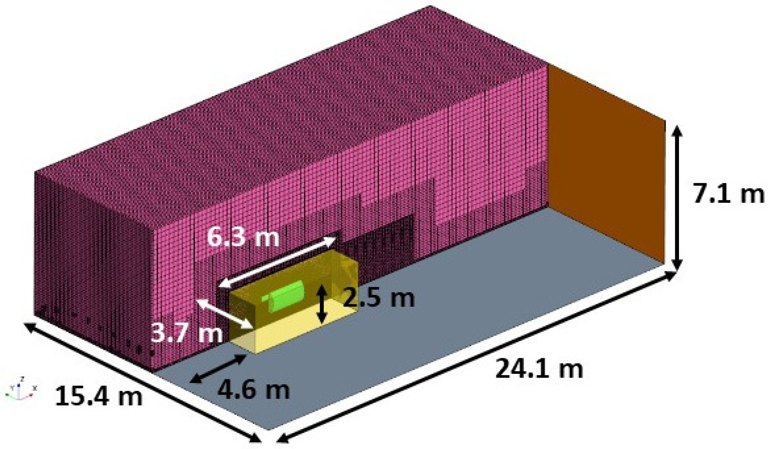
2.4. Validation with a Small AOZ

A small AOZ of ten cows was created to test the performance of the porous cow model. Six cows were lying on the floor, and four cows were standing. This follows the 60/40 ratio for the natural lying and standing behaviour of the cows [2]. They are randomly positioned at different angles to the incoming airflow. For the air, an ambient temperature of T₀ = 9 °C was chosen to also test the interpolation. In addition, different inlet velocities were chosen to account for the velocity dependence of the regression curves. The inlet velocities are 0.5 m·s⁻¹, 1.5 m·s⁻¹, and 3.0 m·s⁻¹.

All simulations were carried out with the solid and porous cows in a steady state. The numerical models and meshing methods are those described above. Figure 6 shows the simulation domain and the measurements. The height of the simulation domain in the z-direction is 7.9 m, and the height of the AOZ box is 1.7 m.

To compare the results, the authors looked at the temperature distribution on the outlet surface and on a horizontal plane through the simulation domain. The pressure drop across the entire AOZ using the mass-flow-averaged total pressure was also examined and compared. Moreover, the evaluation of the pressure drop behind the AOZ for different distances to the end of the AOZ was investigated. Therefore, a distance measure was used, which is defined in Equation (8) as follows:

$${\displaystyle \frac{\mathrm{d}\mathrm{W}}{\mathrm{W}}}={\displaystyle \frac{\mathrm{S}-\mathrm{W}}{\mathrm{W}}}$$

(8)

Here, W is the width of the AOZ in the x-direction, and S is the distance in the x-direction from the beginning of the AOZ. A visualization can be seen in Figure 7.

3. Results and Discussion

3.1. Results for Pressure Drop

Figure 8 shows the results for the pressure drop per length in Pa·m⁻¹ of the single solid cow model as a function of the cow position, flow direction, and wind speed.

For all cow positions and wind directions, the pressure drop increases with increasing flow velocity. This behaviour was also observed by [2]. The pressure drop is highest for the lying cow in cross flow and lowest for the standing cow in front flow. In general, it is higher for the cross flow for both cow positions. This is due to the greater surface area exposed to the airflow. This leads to higher turbulence behind the cow and therefore to a higher pressure drop [13]. In all cases, the pressure drop for the lying cow exceeds that of the standing cow, especially at the higher velocities in the cross flow. This could be due to its position within the boundary layer on the ground. This leads to a lower total pressure downstream of the cow, resulting in a higher pressure drop.

Figure 9 shows the resulting resistance coefficients, P_i and P_v, for the porous cow model as a function of the simulated pressure drop. It can be seen that the resistance values for the cross flow are higher than those for the front flow. This is due to the higher pressure drop they have to account for. For higher flow velocities, the P_v values appear to plateau. This could be due to the decreasing influence of viscosity versus inertia.

In general, the curves reflect the behaviour of the pressure drop found with the solid cow model. The corresponding logarithmic trend lines for the porous cow are shown in

Table 1. Trend lines for the porous resistance coefficients depending on cow posture, wind speed, and flow direction.

Cow Position and Flow Direction	Trend Line	R2
Lying, cross	${\mathrm{P}}_{\mathrm{i},\mathrm{l}\mathrm{c}}=0.15\cdot \mathrm{l}\mathrm{n}\left({\mathrm{v}}_{\mathrm{y}}\right)+0.33$	0.98
	${\mathrm{P}}_{\mathrm{v},\mathrm{l}\mathrm{c}}=0.16\cdot \mathrm{l}\mathrm{n}\left({\mathrm{v}}_{\mathrm{y}}\right)+0.31$	0.98
Standing, cross	${\mathrm{P}}_{\mathrm{i},\mathrm{s}\mathrm{c}}=0.11\cdot \mathrm{l}\mathrm{n}\left({\mathrm{v}}_{\mathrm{y}}\right)+0.28$	0.91
	${\mathrm{P}}_{\mathrm{v},\mathrm{s}\mathrm{c}}=0.11\cdot \mathrm{l}\mathrm{n}\left({\mathrm{v}}_{\mathrm{y}}\right)+0.28$	0.89
Lying, front	${\mathrm{P}}_{\mathrm{i},\mathrm{l}\mathrm{f}}=0.02\cdot \mathrm{l}\mathrm{n}\left({\mathrm{v}}_{\mathrm{x}}\right)+0.04$	0.97
	${\mathrm{P}}_{\mathrm{v},\mathrm{l}\mathrm{f}}=0.02\cdot \mathrm{l}\mathrm{n}\left({\mathrm{v}}_{\mathrm{x}}\right)+0.04$	0.97
Standing, front	${\mathrm{P}}_{\mathrm{i},\mathrm{s}\mathrm{f}}=0.01\cdot \mathrm{l}\mathrm{n}\left({\mathrm{v}}_{\mathrm{x}}\right)+0.04$	0.98
	${\mathrm{P}}_{\mathrm{v},\mathrm{s}\mathrm{f}}=0.02\cdot \mathrm{l}\mathrm{n}\left({\mathrm{v}}_{\mathrm{x}}\right)+0.04$	0.96

. The associated R² values indicate a good fit for each selected trend line.

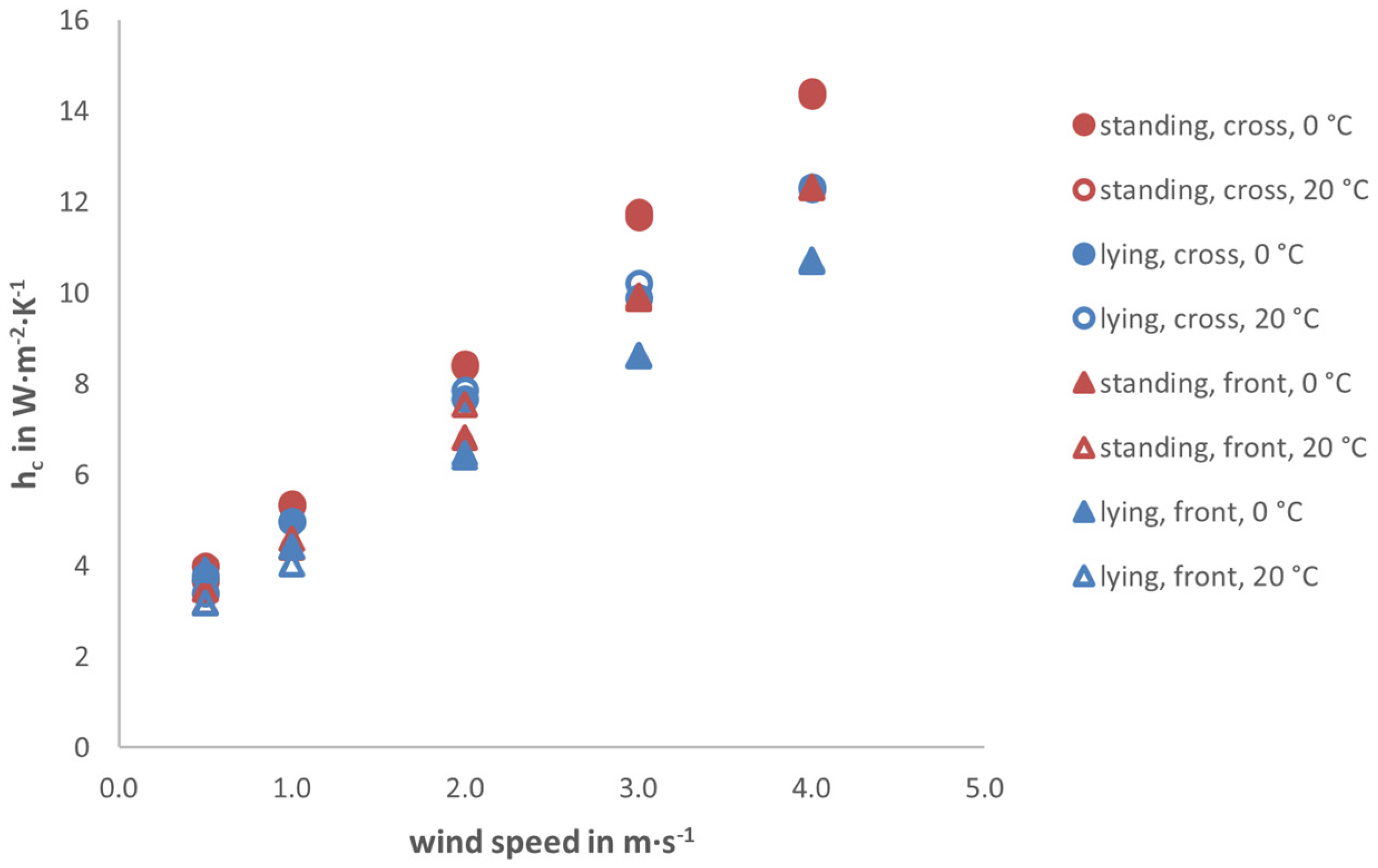
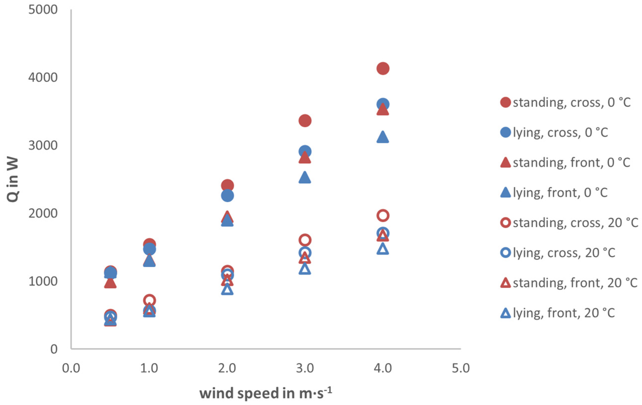
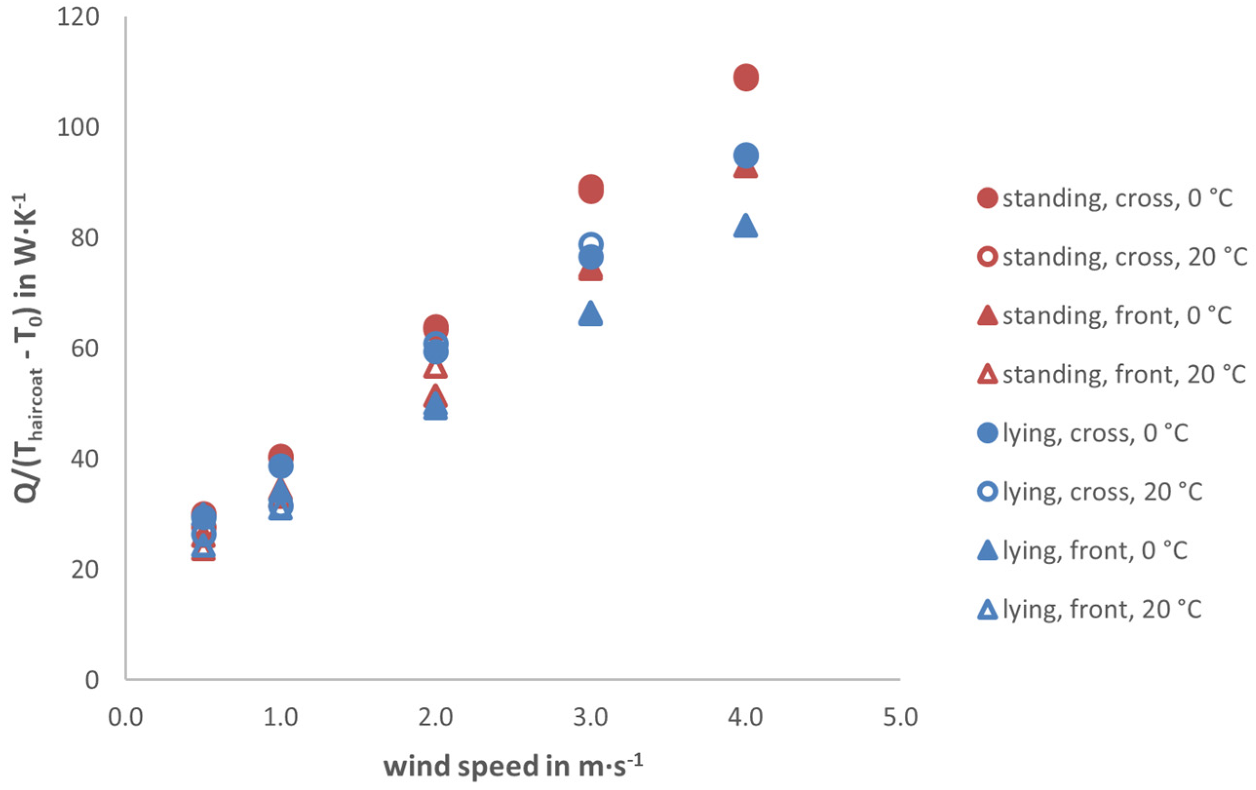
3.2. Results for Heat Transfer

The results for the Nusselt number of the solid cow model as a function of cow posture, wind speed, and flow direction are shown in Figure 10 for the two ambient temperatures of T₀ = 0 °C and T₀ = 20 °C, respectively.

The Nusselt number is highest for a standing cow in a cross flow and lowest for a lying cow in a front flow. The other two combinations of cow position and wind direction are in between. They show almost the same values per ambient temperature. It can also be seen that the Nusselt number increases with increasing wind speed. This means that the amount of convective heat transfer increases, which was also observed by Wang et al. [13]. In addition, the Nusselt number is always slightly higher for the lower ambient temperature. This shows that there is a higher heat flux between the environment and the heat exchanger when there is a higher temperature difference between them.

Wang et al. [13] found a relationship between the Nusselt number and the Reynolds number (i.e., the flow velocity) for a single cow depending on the position of the cow and the wind direction for an ambient temperature of 25 °C. The results shown in Figure 10 are in the same range. Similarly, the cross-flow cases are the ones with the higher Nusselt number due to the higher turbulence intensity leading to a higher heat transfer rate [19].

Furthermore, the magnitude of the values is similar to that of [13], although slightly higher. The characteristic length was calculated using the modified body weight, which might still bias the results. In particular, the lying cow is designed in a different way. Here, the standing cow model was transferred in the z-direction, whereas [13] used a completely different cow model for this case with different measurements but still with the same weight and therefore the same characteristic length. In addition, Wang et al. [13] used 38.7 °C as the haircoat temperature, whereas in this paper, 38 °C was used as reported by [20].

With the aforementioned relationship between the Nusselt number, Nu, and h_c (see Equation (5)), it is now possible to derive the h_c distribution for the two temperature roots. This can be seen in Figure 11.

These parameters show a linear increase with increasing flow velocity. The values vary between 3.18 W·m⁻²·K⁻¹ for the lying cow facing a front flow of 0.5 m·s⁻¹ at 20 °C and 14.42 W·m⁻²·K⁻¹ for a standing cow in a cross flow of 4.0 m·s⁻¹ at the same temperature. These values are in the range of those reported by [2] for a whole AOZ. The influence of the change in ambient temperature can hardly be seen in the resulting heat transfer coefficient values. For this reason, only the variations in cow position and direction of flow are taken into account for the regression formulae. This leads to the equations for the heat transfer coefficient, h_c, listed in

Table 2. Trend lines for the heat transfer coefficient, h_c, in W·m⁻²·K⁻¹ for different cow postures and flow directions.

Cow Position and Flow Direction	Trend Line	R2
standing, cross	${\mathrm{h}}_{\mathrm{c},\mathrm{s}\mathrm{c}}=3.05\cdot \left|{\mathrm{v}}_{\mathrm{y}}\right|+2.33$	0.99
lying, cross	${\mathrm{h}}_{\mathrm{c},\mathrm{l}\mathrm{c}}=2.49\cdot \left|{\mathrm{v}}_{\mathrm{y}}\right|+2.50$	0.99
standing, front	${\mathrm{h}}_{\mathrm{c},\mathrm{s}\mathrm{f}}=2.60\cdot \left|{\mathrm{v}}_{\mathrm{x}}\right|+1.99$	0.99
lying, front	${\mathrm{h}}_{\mathrm{c},\mathrm{l}\mathrm{f}}=2.09\cdot \left|{\mathrm{v}}_{\mathrm{x}}\right|+2.32$	0.99

. These results represent the mean value of the linear trends for a combination of cow position and flow direction for the respective temperatures from Figure 11. The high R² values confirm the linear progression already seen in Figure 11.

Following the procedure outlined in Figure 4, the trend lines for the h_c distribution were implemented in the porous cow model. This allowed the corresponding heat flux to be identified for the different boundary conditions. Figure 12 shows the results.

The linear progression of the Nusselt number of the solid cow model (see Figure 10) can also be seen here. The heat flux at the lower ambient temperature is higher than at the higher ambient temperature. The range is from 428 W (standing, front, 20 °C, 0.5 m·s⁻¹) up to 4134 W (standing, cross, 0 °C, 4.0 m·s⁻¹).

In order to make the heat independent of the ambient temperature T₀, it was related to the difference between this parameter and the cow’s haircoat temperature T_haircoat [13]. The resulting distribution for the porous cow model can be seen in Figure 13.

Similar to the heat transfer coefficient, one trend line for each combination of cow posture and flow direction was derived from the dataset. The results are listed in

Table 3. Trend lines for heat flux Q/dT in W·K⁻¹ for different cow postures and flow directions.

Cow Position and Flow Direction	Trend Line	R2
standing, cross	${\mathrm{Q}/\mathrm{d}\mathrm{T}}_{\mathrm{s}\mathrm{c}}=23.19\cdot \left|{\mathrm{v}}_{\mathrm{y}}\right|+17.49$	0.99
lying, cross	${\mathrm{Q}/\mathrm{d}\mathrm{T}}_{\mathrm{l}\mathrm{c}}=19.62\cdot \left|{\mathrm{v}}_{\mathrm{y}}\right|+18.01$	0.99
standing, front	${\mathrm{Q}/\mathrm{d}\mathrm{T}}_{\mathrm{s}\mathrm{f}}=19.67\cdot \left|{\mathrm{v}}_{\mathrm{x}}\right|+14.79$	0.99
lying, front	${\mathrm{Q}/\mathrm{d}\mathrm{T}}_{\mathrm{l}\mathrm{f}}=16.06\cdot \left|{\mathrm{v}}_{\mathrm{x}}\right|+17.86$	0.99

. Again, the associated R² values show a good fit to the linear progression.

3.3. Results for the Validation with a Small AOZ

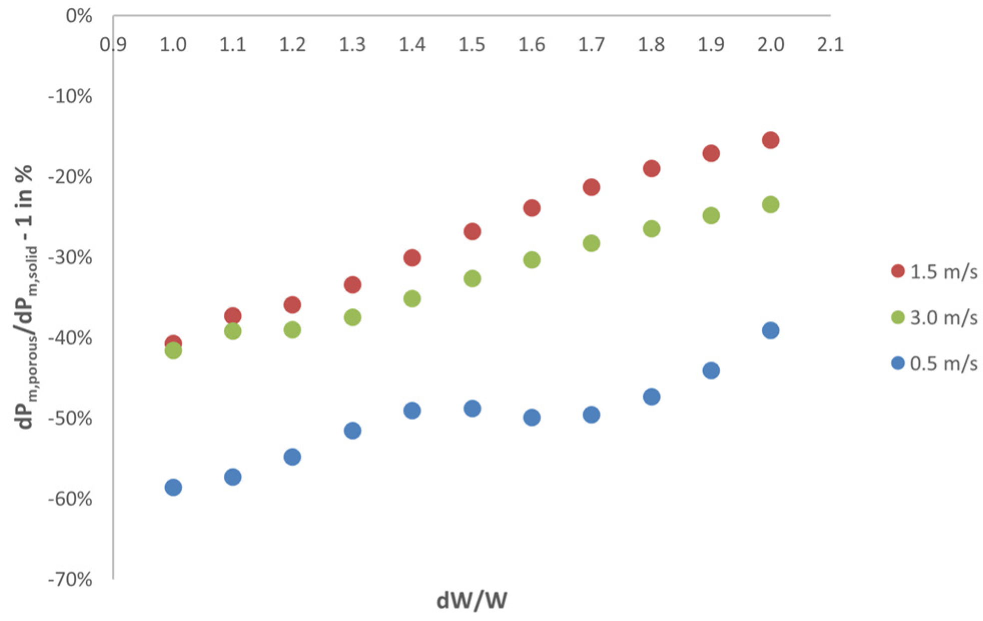
3.3.1. Pressure Drop over the AOZ

When validating the pressure drop, the error between the two model approaches represents the suitability of the model. According to [21], a good agreement is given when the error is less than 10% at most measured points. Agreement is acceptable when the error is between 10% and 30%, marginal when the error is between 30% and 50%, and poor when the error is greater than 50% at most measured points. We have used this definition to grade the results.

Figure 14 shows the development of the relation of the pressure drop behind the AOZ between the solid and the porous model approach. On the x-axis, the distance behind the AOZ is expressed as dW/W (Equation (8)).

The developments of the deviation for the cases with 1.5 and 3.0 m·s⁻¹ are very similar. They decrease from an underestimation of 41% and 42% to an underestimation of 14% and 23%, respectively. Using the suitability measures from [21], the agreement improves from marginal to acceptable. For the case with a flow velocity of 0.5 m·s⁻¹, the deviation changes from −59% to −39%; thus, the agreement changes from poor to marginal. Due to the low flow velocity, the case is dominated by natural convection. The pressure drop for the single-cow model was developed without the influence of temperature; therefore, it is only valid for cases where forced convection is dominant. The development of a pressure drop curve, taking into account the temperature differences between the cow and the surroundings, especially in low-wind-speed situations, should be a task for future improvements of the model.

Figure 15 shows the flow field through the AOZ for the inflow velocity of 3 m·s⁻¹.

It can be seen that the AOZ with the porous cow model cannot capture the strong reversed flows behind the solid modelled cows, as indicated by a very low velocity magnitude near 0 m·s⁻¹. Therefore, the pressure drop evaluated in the close vicinity of the AOZ differs largely between the two model approaches. However, further downstream behind the AOZ, the velocity distribution is very similar between the two model approaches, as can be seen from the pressure distribution in Figure 14.

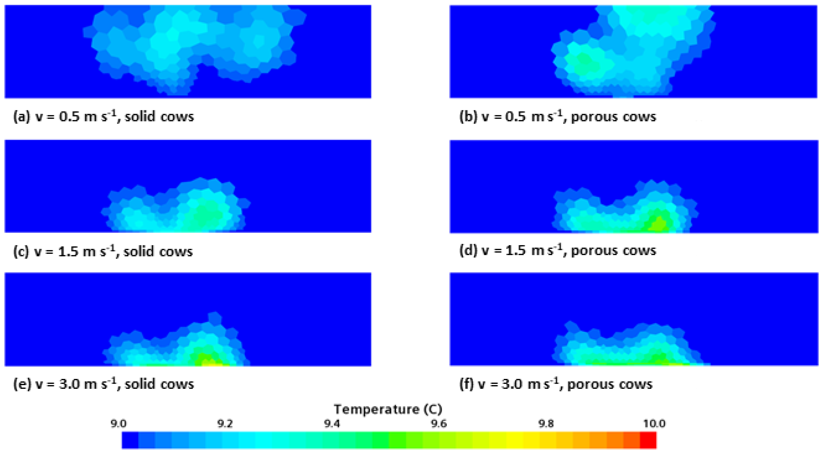
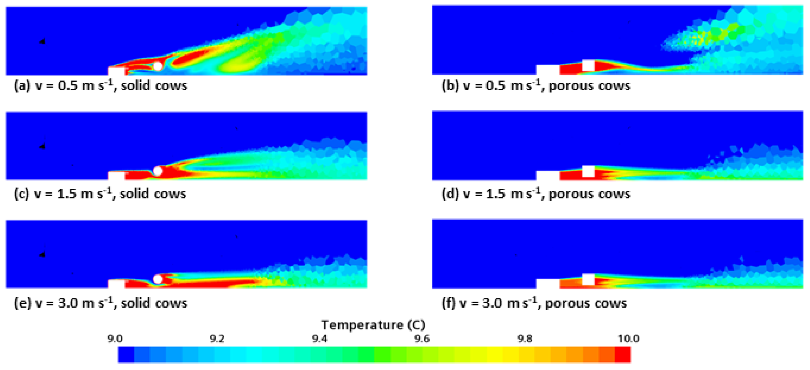
3.3.2. Heat Transfer of the AOZ

The results show very small differences between the solid and the porous cow approaches over the entire velocity range. This shows that interpolation between the 0 °C and 20 °C trend lines gives the corresponding trend lines for the simulated temperature of T₀ = 9 °C. The general behaviour (the higher the flow velocity, the lower the temperature) is also captured by the porous model. However, in all three cases, the porous approach slightly overestimates the temperature at the outlet.

Figure 16 shows the temperature distributions at the outlet of the AOZ simulation domain. On the left-hand side, Figure 16a,c,e show the temperature distribution with the solid cows, and on the right-hand side, Figure 16b,d,f show the distribution with the porous cow models.

It can be seen that the general behaviour of the temperature distribution is maintained by the porous model approach. The higher the flow velocity, the lower the area of high temperature. In addition, as the flow velocity increases, the area of high temperature becomes flatter, which accounts for the straighter streamlines in high velocity flows. However, as the flow velocity increases, a hot spot appears in the temperature distribution of the porous approach (which is especially visible for 1.5 m·s⁻¹). This is due to the lack of turbulent mixing behind the cows. With the solid approach, the cows form a solid obstacle to the flow, which can lead to stalling at sharp edges. It also creates eddies that lead to mixing. This does not happen with the porous approach. The porous block is not a solid obstacle. It simulates the pressure drop and heat transfer according to the parameters found above, but it does not force the creation of turbulent eddies. Figure 17 visualizes this difference between the two model approaches. The mixing, due to turbulence when modelling with the solid cows, can be seen on the left. For the solid cow model, the temperature seems to decrease faster (i.e., closer to the end of the AOZ) than for the porous model approach. For the solid cow model the coloring indicates a temperature around 9.5 °C (green) whereas in the same area of the porous cow model towards the righ-hand side of the figure (b), the temperature is closer to 9.8–10 °C (orange to red coloring).

This effect of the lack of mixing can also be seen when looking at a plane parallel to the flow at y = 12.56 m through the simulation domain. Figure 18 shows this for the case discussed above.

It can be seen that the general behaviour of the temperature distribution is well captured by the porous cows. The flattening of the spatial extent and the generation of the hot spot area can also be seen. Looking at the distribution for the low flow velocity (first row), large differences are visible as the wake region with the porous cow model seems to be non-uniform compared to the one with the solid cow model. To illustrate this, Figure 19 shows a plot of an iso-surface for a temperature of T = 9.5 °C for the two cases. The evaluation plane at y = 12.56 m, as mentioned above, is marked with a solid line for both situations.

It becomes evident that the wake region is very different depending on the model approach for the cows. However, as mentioned above, this case is dominated by natural convection, which is a complicated flow situation on its own. Therefore, it is recommended to further develop the coefficients for the porous cow model so that it can capture cases with natural convection in a better way.

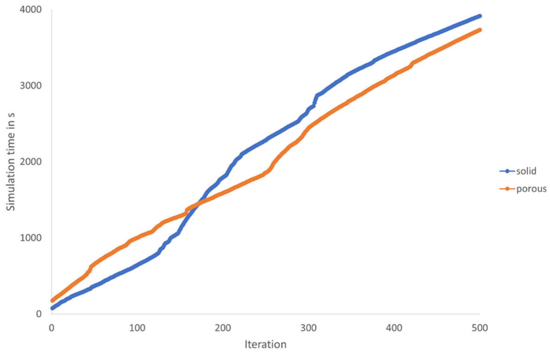
3.3.3. Computational Time and Mesh Size

To obtain another measure of comparison between the two approaches, the computational time and the mesh size were evaluated for the case of 1.5 m·s⁻¹. The mesh count for the two cases is 6,461,440 cells with the solid cow approach and 3,145,117 cells for the porous approach, thus being halved from one model to another. It should be mentioned that the advantages regarding the mesh count should increase further with the number of cows in the model. The number of surface elements in the case used for the solid standing cow model was 20,817. For the porous standing cow model, it was 6348 elements. For the lying cows, the numbers of the elements used were 18,368 and 5744, respectively. For both cow positions, the porous cow model splits the element numbers into thirds approximately. Therefore, the total saving of elements increases with the number of cows in the simulation domain from one model approach to the other.

Figure 20 shows the total simulation time for the two cases. Five hundred iterations take 3915 s with the solid cow approach and 3733 s with the porous cow approach. This is an improvement of 5%.

4. Conclusions

Our study was the first to develop a porous model for a single cow. It was derived from simulations with a single solid cow model. Trend lines were found for the pressure drop and heat transfer coefficients as a function of cow position, wind speed and direction, and ambient temperature for heat transfer. Finally, it was possible to model cow herds with different numbers of animals in a very simple and convenient way to account for their influence.

The single porous cow model approach was validated with simulations using a small random AOZ with single solid cow models. A good agreement was obtained between the two model approaches. It is evident that the single porous cow approach provides a good method for integrating the general influence of the animals into the numerical simulations in terms of pressure drop and heat flux. Furthermore, it is now very convenient to change the number of animals, as it is not necessary to determine the parameters for pressure drop and heat transfer for each AOZ before the actual simulation. It is only necessary to implement the number of animals (porous blocks) in the simulation domain. With the porous model approach, 67% of elements for modelling the cows and approximately 5% of computational time could be saved when simulating a small AOZ of ten animals. The total number of saved elements should increase with the number of cows in the simulation domain. A comparison of the computational time for larger AOZs is up to future research projects. In general, with this model approach, comparisons between whole barns or just cases with different management patterns, animal numbers, or boundary conditions in a naturally ventilated cattle barn can be made in a simpler way.

However, the single porous cow model approach is not suitable for a detailed investigation of the flow pattern and temperature distribution within the AOZ or directly around it. The lack of solid cow geometry leads to simplifications in the vicinity of the animals. Therefore, evaluations should be carried out in a more general and volumetric manner.

The author suggests further investigations of this model. Among other things, wind tunnel tests with cow models and a precise evaluation of pressure drop and heat transfer in the vicinity of a single cow and a herd are conceivable.

References

1. Janke, D.; Yi, Q.; Thormann, L.; Hempel, S.; Amon, B.; Nosek, Š.; van Overbeke, P.; Amon, T. Direct Measurements of the Volume Flow Rate and Emissions in a Large Naturally Ventilated Building. Sensors 2020, 20, 6223. [Google Scholar] [CrossRef] [PubMed]
2. Doumbia, E.M.; Janke, D.; Yi, Q.; Amon, T.; Kriegel, M.; Hempel, S. CFD modelling of an animal occupied zone using an anisotropic porous medium model with velocity depended resistance parameters. Comput. Electron. Agric. 2021, 181, 105950. [Google Scholar] [CrossRef]
3. Bjerg, B. Modelling and Design of the Microclimate in Livestock Housing. In Encyclopedia of Smart Agriculture Technologies; Zhang, Q., Ed.; Springer International Publishing: Cham, Switzerland, 2022; pp. 1–15. ISBN 978-3-030-89123-7. [Google Scholar]
4. Saha, C.K.; Yi, Q.; Janke, D.; Hempel, S.; Amon, B.; Amon, T. Opening Size Effects on Airflow Pattern and Airflow Rate of a Naturally Ventilated Dairy Building—A CFD Study. Appl. Sci. 2020, 10, 6054. [Google Scholar] [CrossRef]
5. Tomasello, N.; Valenti, F.; Cascone, G.; Porto, S.M.C. Development of a CFD Model to Simulate Natural Ventilation in a Semi-Open Free-Stall Barn for Dairy Cows. Buildings 2019, 9, 183. [Google Scholar] [CrossRef]
6. Gautam, K.R.; Rong, L.; Iqbal, A.; Zhang, G. Full-scale CFD simulation of commercial pig building and comparison with porous media approximation of animal occupied zone. Comput. Electron. Agric. 2021, 186, 106206. [Google Scholar] [CrossRef]
7. Bustos-Vanegas, J.D.; Hempel, S.; Janke, D.; Doumbia, M.; Streng, J.; Amon, T. Numerical simulation of airflow in animal occupied zones in a dairy cattle building. Biosyst. Eng. 2019, 186, 100–105. [Google Scholar] [CrossRef]
8. Wu, W.; Zhai, J.; Zhang, G.; Nielsen, P.V. Evaluation of methods for determining air exchange rate in a naturally ventilated dairy cattle building with large openings using computational fluid dynamics (CFD). Atmos. Environ. 2012, 63, 179–188. [Google Scholar] [CrossRef]
9. Iqbal, A.; Gautam, K.R.; Zhang, G.; Rong, L. Modelling of animal occupied zones in CFD. Biosyst. Eng. 2021, 204, 181–197. [Google Scholar] [CrossRef]
10. Stamou, A.; Katsiris, I. Verification of a CFD model for indoor airflow and heat transfer. Build. Environ. 2006, 41, 1171–1181. [Google Scholar] [CrossRef]
11. Rong, L.; Nielsen, P.V.; Bjerg, B.; Zhang, G. Summary of best guidelines and validation of CFD modeling in livestock buildings to ensure prediction quality. Comput. Electron. Agric. 2016, 121, 180–190. [Google Scholar] [CrossRef]
12. Zhai, Z.J.; Zhang, Z.; Zhang, W.; Chen, Q.Y. Evaluation of Various Turbulence Models in Predicting Airflow and Turbulence in Enclosed Environments by CFD: Part 1—Summary of Prevalent Turbulence Models. HVACR Res. 2007, 13, 853–870. [Google Scholar] [CrossRef]
13. Wang, X.; Zhang, G.; Choi, C.Y. Effect of airflow speed and direction on convective heat transfer of standing and reclining cows. Biosyst. Eng. 2018, 167, 87–98. [Google Scholar] [CrossRef]
14. Wu, X.; Shi, Z.; Li, H. Study on the air resistance of pigs in groups based on open-source CFD code: Influence of stocking density and live weight. Biosyst. Eng. 2022, 220, 1–18. [Google Scholar] [CrossRef]
15. Mondaca, M.; Choi, C. An Evaluation of Simplifying Assumptions in Dairy Cow Computational Fluid Dynamics Models. Trans. ASABE 2016, 59, 1575–1584. [Google Scholar] [CrossRef]
16. Siemens Digital Industries Software. How to Monitor the Pressure Drop. Available online: https://support.sw.siemens.com/knowledge-base/KB000036373_EN_US (accessed on 25 April 2023).
17. Marek, R.; Nitsche, K. Praxis der Wärmeübertragung Grundlagen—Anwendungen-Übungsaufgaben; Carl Hanser Verlag GmbH & Co KG: München, Germany, 2015; ISBN 978-3-446-46124-6. [Google Scholar]
18. Heinrichs, A.J.; Rogers, G.W.; Cooper, J.B. Predicting body weight and wither height in Holstein heifers using body measurements. J. Dairy Sci. 1992, 75, 3576–3581. [Google Scholar] [CrossRef] [PubMed]
19. Li, H.; Rong, L.; Zhang, G. Study on convective heat transfer from pig models by CFD in a virtual wind tunnel. Comput. Electron. Agric. 2016, 123, 203–210. [Google Scholar] [CrossRef]
20. Mader, T.L.; Davis, M.S.; Kreikemeier, W.M. Case Study: Tympanic Temperature and Behavior Associated with Moving Feedlot Cattle. Prof. Anim. Sci. 2005, 21, 339–344. [Google Scholar] [CrossRef]
21. Zhang, Z.; Zhang, W.; Zhai, Z.J.; Chen, Q.Y. Evaluation of Various Turbulence Models in Predicting Airflow and Turbulence in Enclosed Environments by CFD: Part 2—Comparison with Experimental Data from Literature. HVACR Res. 2007, 13, 871–886. [Google Scholar] [CrossRef]
Figure 1. Measurements of the solid cow model (ac); evaluation box of the solid cow and porous block of the porous cow model (df).
Fluids 10 00142 g001
Figure 2. Flow chart for finding the resistance coefficients of the single porous cow model depending on cow position, wind direction, and speed.
Fluids 10 00142 g002
Figure 3. Measurements and volume mesh of the simulation domain for finding the pressure drop of the solid cow model and for the design study for determining the resistance coefficients of the porous cow model.
Fluids 10 00142 g003
Figure 4. Flow chart for finding the heat transfer coefficient, hc, in W·m−2·K−1 and the heat flux, Q, in W of the single porous cow model depending on cow position, wind direction, and speed.
Fluids 10 00142 g004
Figure 5. Measurements and volume mesh of the simulation domain for finding the Nusselt number, Nu, of the single solid cow model.
Fluids 10 00142 g005
Figure 6. Dimensions and surface mesh of the simulation domain for the comparison of the solid and porous cow models in a small AOZ: (a) view of the whole simulation domain; (b) detailed view of the AOZ.
Fluids 10 00142 g006
Figure 7. Definition of variables S and W for the derivation of parameter dW/W.
Fluids 10 00142 g007
Figure 8. Pressure drop per length in Pa·m−1 depending on cow position, flow direction, and wind speed for the solid cow model.
Fluids 10 00142 g008
Figure 9. Resulting values for resistance coefficients for the porous cow model: (a) inertial resistance coefficient Pi in kg·m−4; (b) viscous resistance coefficient Pv in kg·m−3·s−1.
Fluids 10 00142 g009
Figure 10. Relationship for the solid cow model between the Nusselt number, Nu, and wind speed for different cow postures, flow directions, and ambient temperatures.
Fluids 10 00142 g010
Figure 11. Relationship between heat transfer coefficient hc in W·m−2·K−1 and wind speed for two ambient temperatures, T0 = 0 °C and T0 = 20 °C, and different cow postures and flow directions.
Fluids 10 00142 g011
Figure 12. Relationship between the emitted heat of the porous cow model, Q, in W, depending on cow posture, wind speed, flow direction, and ambient temperature.
Fluids 10 00142 g012
Figure 13. Distribution of the heat dissipation of the porous cow model in W·K−1 depending on cow posture, wind speed, flow direction, and ambient temperature.
Fluids 10 00142 g013
Figure 14. Change in the deviation of the pressure drop, dP, across the AOZ as a function of the distance downstream of the AOZ for different flow velocities; 1.0 dW/W is at the end of the AOZ.
Fluids 10 00142 g014
Figure 15. Flow field through the AOZ for a wind speed of 3 m·s−1 for an ambient temperature of 9 °C at a height of 0.6 m: (a) solid cow model approach; (b) porous cow model approach.
Fluids 10 00142 g015
Figure 16. Comparison of temperature distribution on the simulation domain outlet for different inflow velocities through the AOZ at T0 = 9 °C: left-hand side (a,c,e), solid cow approach; right-hand side (b,d,f), porous cow approach; top row (a,b), 0.5 m·s−1; middle row (c,d), 1.5 m·s−1; bottom row (e,f), 3 m·s−1.
Fluids 10 00142 g016
Figure 17. Visualization of the flow stream through the small AOZ with respect to the temperature in °C at a height of z = 0.6 m for a flow velocity of 1.5 m·s−1 and an ambient temperature of T0 = 9 °C: (a) solid cow model; (b) porous cow model.
Fluids 10 00142 g017
Figure 18. Comparison of temperature distribution on a plane (y = 12.56 m) for different inflow velocities through the AOZ at T0 = 9 °C: left-hand side (a,c,e), solid cow approach; right-hand side (b,d,f), porous cow approach; top row (a,b), 0.5 m·s−1; middle row (c,d), 1.5 m·s−1; bottom row (e,f), 3 m·s−1.
Fluids 10 00142 g018
Figure 19. Iso-surface at T = 9.5 °C and an inflow velocity of 0.5 m·s−1 through the AOZ where T0 = 9 °C: (a) solid cow approach; (b) porous cow approach.
Fluids 10 00142 g019
Figure 20. Comparison of simulation time in s for the two model approaches of solid and porous cows; v = 1.5 m s−1.
Fluids 10 00142 g020