Abstract
Waves on graphs are a current subject of research interest. As opposed to flows on graphs, the reflection–transmission of waves at the graph’s vertex is a problem that needs to be further modelled mathematically. The literature on the reflection and transmission of waves at a vertex is scarce. Some articles are reviewed and discussed. Water waves are a good topic for comparing different mathematical models, from hyperbolic conservation laws to weakly nonlinear, weakly dispersive systems of partial differential equations on a two-dimensional fattened (thick) graph and the respective one-dimensional graph-model reduction. In this study, we present a particular water wave model in which junction angles are systematically included in the mathematical model. Comparing the solutions with the fattened-graph model gave rise to a more general compatibility condition at the vertex. Current research topics of interest are outlined at the end.
1. Introduction
Water waves are a topic of great importance in environmental modelling, as well as in the mathematical modelling and theory of partial differential equations (PDEs). Applications range from surface and internal waves in the ocean to waves in rivers or canal networks. Water waves are also of great importance in Mathematics, where they can represent many challenging problems in a range of areas, from Analysis to mathematical modelling and computing. As an area of PDEs, they can range from hyperbolic conservation laws to nonlinear, dispersive wave equations. From linear to nonlinear equations, constant or variable coefficients, containing local or nonlocal (differential or pseudo-differential) operators, may be present. Namely, a rich and broad area of PDEs, in which water waves on graphs is quite unexplored, will be reported here.
Irrespective of the fluids’ application, flow on graphs is a topic of current mathematical interest. It falls in a category of problems which has attracted a great deal of attention recently: quantum graphs. Quantum graphs are defined as metric graphs equipped with a differential equation along it’s edges [1,2,3]. Very recently, Goodman et al. [4] published an article pointing to a MATLAB (version R2023b) package for computations on quantum graphs, mostly specialized for elliptic problems. Goodman et al. present a brief introduction to quantum graphs, containing many references to recent work. The mathematical literature on wave propagation on graphs is not as abundant as for flows on graphs [5,6] or steady waves on graphs [1]. It is almost inexistent for wave reflection and transmission at the forked region.
The present article calls attention to wave models on graphs, discussing two modelling levels, where solutions of 2D thick graphs (fattened graphs) and 1D graphs should be compared. As displayed in Figure 1, the thick-graph domain has a small lateral width B when compared to the wavelength (or pulse-width) . The 1D graph, depicted in red, has a vertex (a node) where compatibility conditions need to be imposed.
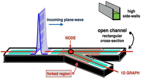
Figure 1.
A schematic picture for the geometrical setting of this water-waves problem: a 2D open channel has a water-wave pulse propagating towards the forked region from the left. The black side-walls of the channel are provided for better visualization. The reduced 1D model is defined on the graph (in red) with a dot at its vertex (node), which will be denoted as P.
Another important point calls attention to diverse applications of waves in graphs. To the best of our knowledge, there are no articles in the literature which present a systematic modelling of branching angles into the 1D-graph’s PDEs. Actually, the majority of the models encountered in the literature do not take angles into account, which for water waves, among other applications, is very important to consider. Moreover, we are not aware of any article that performs a comprehensive comparison between solutions of the parent 2D system of PDEs with those of the reduced 1D system. As reported below, some authors comment on the importance of such a comparative study. The solutions for the reflection–transmission of waves at the forked region are not always in agreement. By comparing solutions on different domains (2D×1D) Nachbin and Simões [7] deduced a new compatibility condition that generalizes the (well-established) Neumann–Kirchhoff conditions [1,3].
2. The Mathematical Background of Water Waves on Graphs
In this section, we present the basic equations for water waves on graphs and review some of the existing articles relating to fluid dynamics on graph-like domains. We also discuss some articles of interest from waves on graphs that are not fluid dynamics-related.
In 1981, Wu [8] worked with Euler equations using the potential theory framework by considering an inviscid fluid flow to be incompressible and irrotational in an open channel. The 3D fluid domain is displayed in detail in the upper-right of Figure 1. The open channel has a rectangular cross-section with high side-walls so that there is no spillage from the channel. The velocity potential satisfies the 3D Laplace equation in , the time-dependent fluid body (in green), together with two nonlinear free surface conditions along the wave elevation . At the impermeable side walls and flat bottom, a homogeneous Neumann condition has to be satisfied. The velocity field in the bulk of the fluid is given by . The 3D potential theory equations are [8,9]:
The (outward) normal derivative in (4) indicates a lack of flow through the impermeable boundaries. Initial conditions are provided along the free surface where the evolution operators are imposed: is the initial free surface disturbance, defining the initial domain configuration , while is the Dirichlet data for the harmonic function to be defined in the bulk.
Through a depth-averaged asymptotic model reduction of the Euler equations, Wu [8] formulated the following weakly nonlinear, weakly dispersive Boussinesq system:
For simplicity, we have used the notation and denoted the reduced potential as . The reduced potential is not a harmonic function, or else the term in (5) would vanish. Therefore it is different from full velocity potential given earlier in system (1)–(4). It is a reduced velocity potential in the sense that the 2D horizontal velocity field is given by . The system has been normalized to have a unit shallow water speed.
This Boussinesq system (5) and (6) was used in the only paper on forked channel regions we are aware of, for nonlinear, dispersive water waves. Shi et al. [10] considered a Y-shaped thick-graph, as depicted in Figure 1. No systematic reduction to a 1D graph-model was attempted in [10], or elsewhere. It is also worth mentioning an earlier work by the group [11] which focused on solitary waves on significantly curved channels. Using Cartesian coordinates, the authors were only able to perform numerical simulations for branching angles that were multiples of . In these cases, the finite difference nodes fell properly along the walls of the secondary channel reaches, as depicted in the schematic Figure 2. Otherwise, one needed to scale the - grid accordingly with the branching angle of the reach. But in the case of two branching reaches at different angles, this strategy would fail.
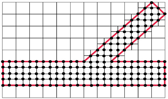
Figure 2.
A schematic picture for a finite difference grid in the physical domain. The red lines depict the channel boundaries while the black circles the nodes for the finite difference scheme.
At the corners of the branching region, one has singularities. In their appendix, Shi et al. [10] report an averaging strategy at corner nodes of the branching region, in order to deal with the lack of a well-defined normal state for the Neumann condition at the side walls. The averaging strategy, using two other neighboring nodes, worked well for channels of moderate width. As the channel widths became smaller, numerical spikes were observed in the simulations. These spikes remained localized near the corner, and would not propagate away.
Next, we present a series of model reductions. We restrict Equations (5) and (6) to a one-dimensional domain:
Then, we differentiate (8) with respect to x. By the definition of the velocity potential, we substitute , and the system can be rewritten as follows:
This is a nonlinear, dispersive Boussinesq system. This system can be further specialized to unidirectional waves, propagating to the right [9]. To obtain the leading order in nonlinearity and dispersion, one can formulate the Korteweg–de Vries (KdV) equation
or the Benjamin–Bona–Mahony (BBM) equation
Equations (11) and (12) allow for solitary (travelling) waves solutions. System (9) and (10) allows for solitary waves in an approximate fashion [11]. Let the total water depth be , where we can set as the normalized undisturbed depth. Drop the (third-order) dispersive term in (10) to obtain the hyperbolic system
We have therefore briefly outlined a modelling hierarchy which started with a 3D, fully dispersive, nonlinear potential theory formulation, and ended with a 1D hyperbolic system. This hyperbolic system is the starting point for our review on a few references for water waves on graphs.
2.1. Fluid Flow Problems on a Graph
We begin by reviewing a few papers we have encountered which relate to fluid flow on graphs. The shallow water (long wave) model presented by Jacovkis [6] was the starting point for our interest in this topic. Two typical junction configurations are considered as shown in Figure 3.
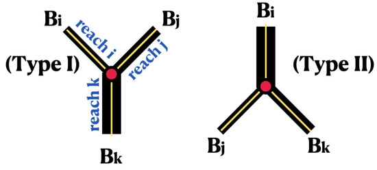
Figure 3.
Two typical junction configurations are considered. A converging junction is indicated as type I and a diverging junction as type II. The reaches’ widths are respectively denoted by , which can be different from each other. The thinner yellow lines represent the graph’s edges. The thicker black rectangles highlight the different widths associated with each reach of the 1D model. The (red) circle indicates the vertex P where compatibility conditions must be applied to the graph solutions along the one-dimensional segments.
Jacovkis [6] considers the following PDE-system of conservation laws:
As opposed to the process described above for the hyperbolic system, now, the wave speed is not normalized and will depend on g, which is the acceleration due to gravity. This is a dimensional version and the shallow water speed is , which is not necessarily equal to 1. This is a strictly hyperbolic system with two real eigenvalues for the system’s matrix
Consider junction configurations such as those displayed in Figure 3. Jacovkis presents a theorem for the linear model in the subcritical regime, where one characteristic points upstream while the other points downstream. The slope of the characteristics are given by the eigenvalues and , where U and H are (constant) reference values for the velocity and depth. The linear shallow water system has the form
Along each reach, we consider the initial conditions
where x is a local coordinate within the respective reach. The Neumann–Kirkhhoff compatibility conditions are as follows:
At the vertex P, the respective reach coordinate is , and . The widths of the respective reaches are displayed in Figure 3 and denoted by , index . Conservation of mass is given by (20), while a first approximation for conservation of momentum is expressed by the continuity of water elevation (21). For simplicity, we now drop the tilde from the velocity and water height perturbations and . Jacovkis considers a type-I junction, as depicted in Figure 3, in order to present the following theorem.
Theorem 1
([6]). Consider the linear shallow water system (18), with initial conditions (19) along each reach, satisfying the Neumann–Kirchhoff compatibility conditions (20) and (21) at the junction point P, together with boundary conditions
at each open extreme point of the Y-shaped network. This problem has a unique solution , at each reach, provided that the following condition apply:
- (i)
- and all the are and consistent with the initial conditions at ;
- (ii)
- the matrix A has real eigenvalues ;
- (iii)
- and are 0/1 binary variables, such that .
- The solution exists for all times .
We outline some points from the proof, which are relevant for our discussion. The matrix A is diagonalizable, with
System (18) can be rewritten as two decoupled wave equations for each component of , where :
Consider the Neumann–Kirchhoff compatibility conditions (20) and (21) at the vertex P, with reaches i and j merging onto reach k, in the Y-configuration, type-I. We state that , and are incoming modes at the vertex, while , and are the respective outgoing modes. The compatibility conditions yield a functional relation between input and output from the vertex P:
The input (incoming modes) appear on the right. Recall that , and are the widths of the respective reaches . It is straightforward to show that theses matrices are nonsingular, so that one can write
is a scattering matrix for the vertex, mapping incoming information to outgoing information. The linear system of Equation (25) indicates that the linear hyperbolic system, defined on this Y-shaped channel region, has a solution. Mathematically, the compatibility conditions allow us to connect the solutions from three different half-lines (semi-infinite reaches).
But this model does not have any information regarding the angles between reaches at the junction. This is an interesting wave model on a graph, which is well defined mathematically, but incomplete with regard to the effect of angles. For example, the model cannot properly account for the back-flow promoted by wave reflection at the junction. The following simple discussion, to the best of our knowledge, is not considered in the work of Jacovkis [6], nor elsewhere in the literature.
Consider three type-I junctions, as depicted in Figure 4. The configuration of the Y-shaped domain, whether it is symmetric or not, should play a role in the flow distribution along the reaches. Also, this should be applicable for wave reflection, as opposed to a pure streaming flow. As an extreme, consider case (A), which is depicted in Figure 4, and case (C). The incoming reaches (both i and j) have half the width of the outgoing reach k. Imagine case (A) with a very small angle upstream (between reaches i and j). For this case, we should not expect back-flow (wave reflection), as opposed to a T-shaped configuration, where there should be a nontrivial flow upstream. Consider expression (26) with the incoming vector given by . Namely, the flow arriving from reaches i and j is the same (at all times), while there is no upstream flow arriving from reach k. For the case (say, with and , for simplicity) it is straightforward to show that the outgoing vector given by (26) is .
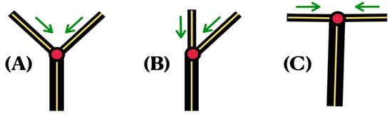
Figure 4.
Three converging-junction configurations: (A) symmetric Y-shaped; (B) asymmetric Y-shaped; (C) T-shaped. The arrows indicate data which enter the vertex P from upstream, without any flow coming from downstream. In all cases, let .
Waves merging onto reach k should generate quite different reflections (and back-flow) in these two extreme cases, as well as the asymmetric case (B) of Figure 4. Comparisons between the 2D fattened-graph model and the 1D simplification help to resolve modelling issues. This was taken into account by Nachbin and Simões [7] for the weakly nonlinear, weakly dispersive PDEs. In Jacovkis [6], as well as many other references, no information relating to angles is built into the models, nor are comparisons drawn between 1D graph-solutions with those of the parent 2D model. It is worth mentioning the paper by Caputo et al. [12], where the authors compared the results of the 2D shallow water equations with its restriction on a graph for a T-junction. The authors report that for the linear case, the Stoker conditions hold, indicating continuity of the wave elevation at the junction point of three reaches with the same width. A wave propagates up the vertical part of the T branch into the two horizontal reaches of the T. The effective width of the fluid domain doubles. Therefore, it is unclear how the wave heights remain the same as they propagate away from each other, while conserving the total excess mass.
The asymmetric configuration of Figure 4B has been addressed through a complex-variables formulation by Milne-Thomson [13]. It is revealing regarding the effect of the branching angle. The 2D shallow water system is of the form
The corresponding linear system is given by
For the fattened (2D) graph-like domain, impose the very simple regime of a steady flow , with no wave elevation, so that . For this regime, system (27)–(29) reduces to the incompressibility condition . Adding the hypothesis of an irrotational flow, , allows for the existence of a velocity potential , such that . Incompressibility implies that the velocity potential is a harmonic function, which has the stream function as its harmonic conjugate, where . Using a complex potential , with , leads to a complex velocity which automatically satisfies the constraints for an incompressible, irrotational flow, due to the Cauchy–Riemann equations for and . Milne-Thomson [13] then uses a sequence of conformal-mapping compositions to express the solution for the streaming flow in an asymmetric junction with angle , as shown in Figure 5. Very quickly, at a small distance away from the branching region, the flow aligns uniformly, parallel to the side walls which have no lateral variations. Milne-Thomson [13] provides the following equation that relates the three limiting uniform speeds along each reach:
Define and consider the case , which yields from the conservation of mass. Equation (30) becomes
This nonlinear equation for the speed ratio in the main reach depends nontrivially on the branching angle . The respective values of are displayed in the top part of Table 1, given a few values of the branching angle. We may also consider the case , which yields . Equation (30) becomes
The respective values of are displayed in the bottom part of Table 1. For simplicity, let , so that columns 5 and 6 in Table 1 give the speeds along the main reach, after the branching point, as well as in the secondary reach. When all reaches have the same width, L, and the branching angle is small, the speed after the forked region falls to half of the incoming value, as shown in the first row of Table 1. In the schematic, Figure 6 the total channel width doubles at the forked region, and therefore the speed is halved so that the flux is maintained. When the widths of the secondary reaches reduce by half (right of Figure 6), the total width remains unchanged, and therefore all speeds are (effectively) the same as shown in the first row of the bottom part of Table 1. In both cases, the speeds and change as the branching angle increases. This shows that the streaming flow, through a (harmonic) velocity potential, captures the effect of a branching angle. Nevertheless, as the angle increases further, the speed in the secondary reach becomes larger than in the main reach. As the angle increases, the flow separatrix, depicted in Figure 5, moves downwards, promoting a smaller flux along the lower part of the channel. We have an ideal fluid that slides along boundaries. No vorticity generation mechanism is present, which likely would occur near the outer corner of the inclined secondary reach. This model also has its limitations, but captures angle variations at the forked region. In our wave model [7], in contrast, we observe that as the angle increases, the preferred wave direction is through the main reach. This will be shown in Section 3.
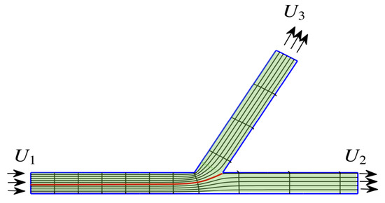
Figure 5.
Streaming flow past an asymmetric forked region at angle . The incoming reach has a width of , while the other two reaches have, respectively, widths of and . The separatrix (red curve), emanating from the forking corner, divides the laminar flow region into two parts: the bottom part, flowing towards the main reach, and the top part flowing towards the secondary reach.

Table 1.
Parameters: .
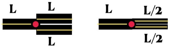
Figure 6.
Two test cases of Table 1, in the small angle limit. Left: when , the total width of the channel doubles. Right: when , the total width of the channel remains the same.
In 2008, Bona and Cascaval [14] presented an analysis of weakly nonlinear, weakly dispersive water waves on 1D graphs. The main application mentioned was blood flow in a branching blood system. The model chosen was the Benjamin–Bona–Mahony (BBM) equation. This is a unidirectional long-wave model which allows for solitary wave propagation. It is a regularized version of the Korteweg–de Vries (KdV) equation. The BBM’s dispersion relation is a Padé approximation of the potential theory’s full dispersion relation [9], which is better equipped to handle the short waves of the solution’s Fourier spectrum.
Let represent the free surface displacement at location x and time t. The BBM equation is defined as [14]
with the Neumann–Kirchhoff conditions at the vertex P, of the flipped Y-domain (type-II in Figure 3):
As mentioned by the authors, in comparison with the KdV equation, the BBM equation seems more amenable to the functional analysis performed, since the number of boundary conditions needed for well-posedness over finite intervals is two, whereas the KdV requires three boundary conditions. The solitary wave profiles for both equations are similar, even though the KdV is an integrable system and the BBM is not.
The above BBM model has no information regarding the angle at a vertex. The authors mention that angles should play a role in the solution, and this is a topic of future interest. A preliminary 1D numerical study is presented at the end of their paper, with the solution displaying reflected waves at the vertex. Wave reflection should be better modeled by a bidirectional PDE system, such as a Boussinesq system. No comparisons are mentioned with 2D solutions in a fattened-graph domain. The functional-analytic study presented [14] is nontrivial and important, and it is necessary to consider the function-space analysis on the half-line for each reach. The authors draw conclusions about the well-posedness of the solutions in its current configuration. As discussed above, the model has limitations but establishes an important step in understanding mathematical aspects of this nontrivial problem of nonlinear evolution equations on a nonstandard domain.
In 2014, Bressan et al. [5] reviewed flows on networks with examples such as traffic flow and blood flow. Their mathematical framework is achieved through conservation laws, in the form of a balance equation such as
where , x is the one-dimensional spatial variable, f is the flow, and g is the forcing term. Results on the existence for solutions are presented for scalar conservation laws as well as systems of conservation laws, where u, f and g are vector quantities. In most cases, the conservation law is equipped with algebraic conditions at the vertices of a directed graph. The authors mention that in most applications considered, there is a preferred direction for the network flow. Section 3.1 in [5], which relates to traffic flow on road networks, reviews different unidirectional traffic flow models and different nodal conditions at the single vertex of the model. The authors comment that the existence and well-posedness properties for the Cauchy problem of incoming roads on a vertex, together with outgoing roads, depend on the choice of the nodal (compatibility) conditions at . The Cauchy problem considers Equation (36) defined on the half-line , together with Equation (36) defined on .
The review in [5] does not discuss information on angles between edges or comparisons with their parent 2D thick-graph model. Bressan et al. present an interesting and extensive analytical review of 1D hyperbolic graph-models. For example, in Section 8 [5] on Future perspectives (page 101), the authors call attention to the importance of imposing proper coupling conditions between different branches of the graph. The consistency of the coupling conditions between edges is very important, where consistency infers comparing with solutions of the full multidimensional problem. Proving that a reduced model is consistent with the higher dimensional one is, in general, an open problem from the rigorous analysis point of view [5]. The rigorous analysis presented in [5] regards 1D solution properties, which are important and nontrivial. Our approach has been to investigate the consistency between the two-level models (1D × 2D) using PDE modelling and theory together with scientific computing. This has led to a novel nonlinear coupling condition at the vertex of the graph. This was performed in Nachbin and Simões [7], where comparisons between the reduced 1D model and the parent model led to a novel and more accurate compatibility condition between edges. This will be discussed in the Results Section 3.
2.2. Non-Fluid Mechanics-Related Problems
Below, we comment on some recent review articles for waves on graphs. We highlight points that call attention to current mathematical problems of interest.
Kuchment [2,3] has written a few review articles (in 2002 and 2008) on quantum graph models for waves in thin structures. We recall the general definition for a quantum graph as a metric graph equipped with a differential equation along its edges, as the present case of water waves. One of the author’s main interests relates to the spectral behavior of some self-adjoint operators on a graph-like domain. It is challenging to understand the convergence of the spectral features in the limiting case when the thin graph-like structure collapses onto a 1D graph, which Kuchment calls a one-dimensional singular variety, also known as the singular nature residing on the presence of a vertex. Mathematically speaking, Kuchment analyses differential operators, such as a Laplace operator, or a Schrödinger operator, with Dirichlet or Neumann boundary conditions, defined on a narrow branching domain. This leads to highly nontrivial problems depending on the graph topology. These questions have attracted the attention of many researchers. Kuchment remarks that vertex conditions can be imposed in different forms, mostly through the Neumann–Kirchhoff condition and some of its variations. The choice of a vertex (compatibility) condition involves prescribing how waves scatter at each vertex. Wave scattering at a vertex sets a difference between flow problems through a vertex, where reflection or a backward flow are less likely to be established by a compatibility condition. This is an important point that we were able to address in the water wave problem by providing vertex conditions together with information on the angle between the respective edges [7].
A recent (2022) review article by Kairzhan, Noja and Pelinovsky [1] considers standing waves of the nonlinear Schrödinger equation on star-shaped quantum graphs. The authors review the existence and stability results for standing waves trapped on quantum graphs. They consider some variations in the Neumann–Kirchhoff condition and mention that angles do not play a role in their applications. Restricting a differential operator to the intervals defined by each edge is trivial. Kairzhan et al. [1] call attention to the ambiguity that can arise through the choice of the compatibility conditions and also that the modelling choices made should be based on the underlying physical problem. This is along the lines of our modelling investigation for the water waves problem. On the other hand, the authors admit that it is unclear which conditions at nodes are appropriate for a good agreement with solutions of the concrete underlying problem. There are different choices that can render a mathematically well-posed problem. But a realistic reduced modelling from the higher-dimensional problem to the one-dimensional metric graph is a fundamental step [1].
The work by Kevrekidis et al. [15] considers matter waves on Y-junctions. The authors also comment on several points which are currently of interest, with an effort to model junction angles. A potential-like term is introduced in a discrete (lattice) nonlinear Schrödinger equation in order to numerically study the effects of graph-asymmetry and of branching angles. This term at the junction is responsible for guiding localized solitary-wave excitations that are studied in the context of optical lattices in Bose–Einstein condensates. They find that the fraction of transmitted condensate may strongly depend on the angle. The authors also comment on the subtleties of one-dimensionality versus small but finite edge-width. And they note that dimensionality comparisons are important and a topic of future investigation.
Many comments from the related works mentioned above corroborate with the direction we have been pursuing: a better understanding of angle modelling for waves on graphs and the effects of dimensionality through a thin fattened-graph and its companion 1D graph. Is the vanishing-edge-width regime a singular limit? In which cases do solutions of the 2D system converge to solutions of the 1D graph? Angles and different compatibility conditions should play a role and need to be investigated more carefully. These are some of the fundamental questions we want to address in ongoing and future work. Water waves represent a proper mathematical setup for this study, where angle modelling, nonlinearity and other features can be added to the PDE study in a natural, physically motivated fashion.
3. Results
In this section, we review our results on weakly nonlinear, weakly dispersive water waves on graphs [7,16]. In particular, we describe how we introduce information about the angles of a forked region in a systematic fashion. The mathematical modelling which improved the compatibility conditions on the vertex of a 1D graph grew out of comparisons with the parent 2D fattened-graph simulations.
In a more general framework, Nachbin and Simões [7,16] used Wu’s Boussinesq system (5) and (6) together with a Schwarz–Christoffel mapping [17], in order to conformally map the physical fluid domain onto a uniform strip. As depicted schematically in Figure 7, the (MATLAB; version R2023b) Schwarz–Christoffel Toolbox [17] maps the canonical domain (on the right) onto the physical domain (on the left). The canonical domain is defined in the complex w-plane (), while the physical domain is defined in the complex z-plane (). The Schwarz–Christoffel mapping is tailored for mapping polygonal-shaped domains; in this case, the forked region shown in Figure 7. The geometrical singularities at the corners of the physical domain are changed in the canonical domain. The outer corner is straightened out and the Jacobian of the coordinate transformation is zero at that point [18]. Clearly, the mapping is not conformal at that point, since it does not preserve the angle. At the inner corner, the Jacobian blows up [18].
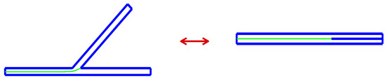
Figure 7.
This is a schematic picture of the Schwarz–Christoffel (SCh) conformal mapping between the physical domain (left) and the canonical domain (right). The physical forked domain is defined in the complex z-plane while the canonical (computational) domain is defined in the complex w-plane. The SCh mapping is defined as . The inverse function maps the forked region onto a uniform strip with a slit. The slit (defined in blue) arises from the conformal mapping having fractional exponents, and therefore a complex function with a branch cut [18]. The slit is connected to the domain’s separatrix, depicted in light green.
In order to avoid the presence of these singularities in our computational domain, we map a (z-plane) domain with a slightly larger width than the desired physical domain. This wider region is shown in Figure 8. We then evaluate the Jacobian on grid points away from the boundary and the singularity. These grid points are those within the forked region bounded by the thick black lines, as depicted in Figure 8. This strategy was tested numerically for both a sharp turn [16] as well as the forked region [7].
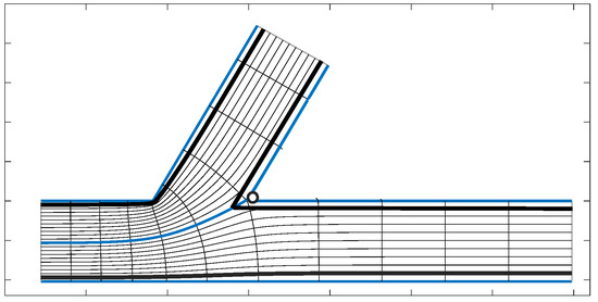
Figure 8.
In order to deal with the conformal mapping’s singularity, we consider a slightly wider forked channel to be mapped by onto a uniform strip in the canonical w-plane, as shown in Figure 7. The Jacobian of this mapping blows up at the corner highlighted with a circle. To avoid the singularity, the physical domain is defined by the slightly smaller region within the region bounded by the thicker inner curves. The mapping’s separatrix is depicted emanating from the singular point. For the numerical simulations, the values of the Jacobian are finite and taken from this inner region, which has the singularity nearby, but outside the domain of interest. This is depicted in Figure 9.
Using the Schwarz–Christoffel Toolbox [17] we evaluate and plot the Jacobian of an asymmetric forked region, as shown in Figure 9. Note that the singularity is felt near the branching region, shown by a spike. But the spike is finite, since the singularity is outside the domain. Away from the forked region, the Jacobian very quickly reaches plateaus of constant value. This is related to the discussion presented together with Figure 5. The roles played by the coordinates and , as functions of the inverse mapping , are analogous to the roles played by and in the steady streaming flow presented by Milne-Thomson [13]. Note that in Figure 5, a short distance away from the forked region, the streamlines (aligned with the walls), together with potential level-curves, form a Cartesian grid. This means that the Jacobian matrix away from the forked region is a constant multiple of the identity. Namely, it is a rotation and/or rescaling of the standard Cartesian coordinates.
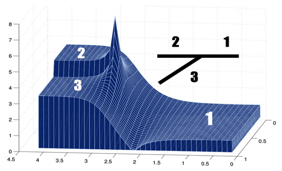
Figure 9.
The Jacobian produced by the Schwarz–Christoffel Toolbox [17]: , by the Cauchy–Riemann equations. At the corner between reaches 1 and 3, the Jacobian is zero. At the corner between reaches 2 and 3, the Jacobian blows up [18].
Bearing the above conformal mapping in mind, we apply this curvilinear, orthogonal change of coordinates to the Boussinesq system formulated by Wu, which we repeat here for convenience:
Recall that the is not a harmonic function, or else the term in the first equation would be zero. This Boussinesq system is not invariant under the Schwarz–Christoffel change of variables. But the -coordinate system is boundary-fitted and the respective Jacobian encodes geometrical angle-information in an algebraic form, through variable coefficients in the system of PDEs. Under the conformal change of coordinates, the variable-coefficient Boussinesq system takes the form
The Jacobian of the Schwarz–Christoffel mapping is given by . As a boundary-fitted coordinate system, it is easy to impose the Neumann conditions along the walls of the secondary reaches. Therefore, forked regions with reaches of different angles are easily treated in our numerical computations, with the discretization being in the (Cartesian) canonical variables. An outline of the numerical scheme used is provided in Section 4.
For the regime of interest (long waves in narrow channels), the 2D fattened-graph simulations displayed solutions which are essentially one-dimensional [7] when they are away from the forked region. The narrow channel is a wave-guide and the water waves propagate as a plane-waves along each reach. The Neumann conditions along the side walls act in this regard, aligning the wavefront with the propagation direction of the reach. This means that away from the forked region, we can disregard lateral variations of the wave. In other words, the -dependence of solutions of the Boussinesq system (37) and (38) can be dropped. With this in mind, a 1D water-wave graph-model was deduced by Nachbin and Simões [7] along the axial direction of the reaches:
The bars denote that these functions do not depend on ; only on . The 1D horizontal velocity along the channel axis is denoted by = , while the wave elevation by . The lateral averaging of the Jacobian is denoted by . In this 1D equation, the Jacobian is taken as a piecewise-constant coefficient which encodes angle-information.
By observing the 2D fattened-graph solution, we see that continuity of the wave elevation does not hold, as clearly depicted in Figure 10. There is a sudden change in wave height at the forking point, and therefore a Rankine–Hugoniot jump condition was imposed in [7]. This jump condition gave rise to our compatibility condition, generalizing the established Neumann–Kirchhoff condition. Writing Equation (40) in divergence form leads to a Rankine–Hugoniot jump condition [7] which is deduced from a stationary shock at the vertex. Rankine–Hugoniot conditions along each reach connection (1-2; 1-3) yield the nonlinear compatibility conditions (41) and (42), which generalize the Neumann–Kirchhoff condition:
is the fluid flux at a given point of the graph, in canonical coordinates. At the vertex P, condition (43) implies conservation of mass, where the indicates the respective endpoint of reach . When the nonlinear terms are discarded from (41) and (42), the Neumann–Kirchhoff condition [1,3] is recovered, which is also called the Stoker condition mentioned by Jacovkis [6]. The Neumann–Kirchhoff condition imposes the continuity of the solution at the graph’s vertex: . Nachbin and Simões [7] (Figure 7) present a numerical simulation with the Neumann–Kirkhhoff (Stoker) condition for a moderate angle of . We compare the 2D solution with the 1D graph-solution. The agreement for the reflected and transmitted waves is not very good. This is particularly true for the reflected wave. Then, in Figure 8 [7], using the new compatibility conditions with the same data as before, the 1D-2D wave reflection-and-transmission agreement is excellent. The new compatibility conditions are further numerically validated by comparing 1D with 2D solutions for different sets of angles and widths [7], in symmetric and asymmetric junctions. A mean-square error analysis for the wave elevation is presented in Figure 11 [7]. It considers different channel widths (all three reaches with or all with ), as well as different forking angles ( and ). This comprehensive 1D-2D comparison of solutions in both directions, for several different junction configurations, is not found in the literature of waves on graphs, including water waves.
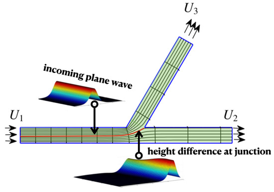
Figure 10.
Snapshots of the abrupt wave-height change while passing through the forked region. The background displays the streaming flow solution [13], which allows less flow () through the horizontal reach. A plane waves approaches the forked region from the left, as shown in the left snapshot. At the forked region, the other snapshot displays a larger wave propagating through the main reach, while a smaller wave is about to propagate through the secondary reach. The two wave profiles, depicted in the snapshots, are from 2D Boussinesq computations by Simões [19]. These wave snapshots clearly illustrate that the Neumann–Kirchhoff condition, which requires continuity of the wave elevation at the forking point, is not a proper condition in this case.
4. Numerical Method for the 2D Boussinesq System
We briefly review the numerical method developed by Nachbin and Simões [16] and used for forked regions in [7]. It is convenient to write system (37) and (38) as follows:
We use centered finite differences for all spatial derivatives, where the grid functions are denoted accordingly, as for example, , at mesh points . Then,
Let the right-hand side of (44) be denoted by and the right hand side of (45) be denoted by :
Define the auxiliary function , which we will use to evolve our ODE system. This function arises from the the time-derivative term in Equation (45). After the ODE solver’s time step, the potential is recovered by solving an elliptic equation at each time step. We start with a predictor scheme for the wave elevation and the auxiliary function:
These values provide an initial guess for the (implicit) corrector scheme. The corrector scheme, at the iteration step , is given by
The iterations are performed until
Once is obtained, we recover the potential from the discrete elliptic problem
with trivial Neumann boundary conditions along the walls. Further details can be found in the work of Nachbin and Simões [16].
The 1D Boussinesq graph-model uses a similar predictor–corrector scheme, also defining an auxiliary function to deal with the dispersion term. Details of the implementation of the compatibility condition are given in the appendix of Nachbin and Simões [7].
5. Discussion and Future Work
Flows on graphs are an interesting research problem discussed in a diverse range of mathematical literature, including some review articles that have been published recently. Here, we commented on two of these articles [1,3]. In contrast with flow on graphs, we called attention to the problem of waves on graphs, where one needs to deal with the reflection and transmission of waves through the vertex of the graph. Existing wave models lack information about the junction’s angles as well as comparisons with the (parent) 2D fattened-graph model. This has an impact on the reflection–transmission dynamics at the vertex of the reduced 1D graph model, and how it compares to the 2D mesoscale model.
As described in Section 2, there are many mathematical problems of interest in the literature which are currently being investigated. These range from PDE modelling, numerical methods and simulations to theoretical studies. In this manuscript, we addressed some issues that are not fully resolved. In order to address some of these interesting questions, we plan to step back from the weakly nonlinear, weakly dispersive Boussinesq system and study (nondispersive) hyperbolic systems. As mentioned in Section 2, this means working with the 2D shallow water equations. To the best of our knowledge, there has not been a comprehensive comparison between thick-Y-graph solutions with that of the reduced (variable angle) 1D tree-like graph, exploring a variety of junction configurations. Also, angles have never been considered systematically in 1D hyperbolic fluid-flow models, and certainly not for shallow water waves on graphs. We believe that linearized systems should take into account junction configurations within the equations. This is currently being addressed in a research project.
Another modelling ingredient of interest is channels with different cross-sections. The Boussinesq model considered in this paper is for a rectangular cross-section, which does not vary along the canal. These are two modelling variations to be considered: (i) non-rectangular cross sections; (ii) spatially varying cross sections.
By no means do we intend to exhaust the list of possibilities, but another topic of interest is the consideration of different types of solutions. Up to now, we have only studied solitary waves. With solitary waves, we observed [7] that the accuracy of the compatibility conditions (41) and (42) deteriorated for an asymmetric junction, as the forking angle was approximately . We want to take a closer look to understand why this loss of accuracy takes place between the 1D and the 2D models.
Funding
The author is on leave from the Instituto de Matemática Pura e Aplicada (IMPA), Brazil. This research was partially funded by the Conselho Nacional de Desenvolvimento Científico e Tecnológico (PQ1D 307078/2021-3) and by Fundação Carlos Chagas Filho de Amparo à Pesquisa do Estado do Rio de Janeiro (CNE E-26/201.156/2021), Brazil.
Conflicts of Interest
The author declares no conflicts of interest.
References
- Kairzhan, A.; Noja, D.; Pelinovsky, D.E. Standing waves on quantum graphs. J. Phys. A Math. Theor. 2022, 55, 2430001. [Google Scholar] [CrossRef]
- Kuchment, P. Graph models for waves in thin structures. Waves Random Media 2002, 12, R1–R24. [Google Scholar] [CrossRef]
- Kuchment, P. Quantum graphs: An introduction and a brief survey. Proc. Symp. Pure Math. 2008, 77, 291–314. [Google Scholar]
- Goodman, R.H.; Conte, G.; Marzuola, J.L. QGLAB: A MATLAB package for computations on quantum graphs. SIAM J. Sci. Comput. 2025, 47, B428–B453. [Google Scholar] [CrossRef]
- Bressan, A.; Canić, S.; Garavello, M.; Herty, M.; Piccoli, B. Flows on networks: Recent results and perspectives. EMS Surv. Math. Sci. 2014, 1, 47–111. [Google Scholar] [CrossRef]
- Jacovkis, P.M. One-dimensional hydrodynamic flow in complex networks and some generalizations. SIAM J. Appl. Math. 1991, 51, 948–966. [Google Scholar] [CrossRef]
- Nachbin, A.; Simões, V.S. Solitary waves in forked channel regions. J. Fluid Mech. 2015, 51, 544–568. [Google Scholar] [CrossRef]
- Wu, T.Y. Long waves in ocean and coastal waters. J. Engng Mech. ASCE 1981, 107, 501–522. [Google Scholar] [CrossRef]
- Whitham, G.B. Linear and Nonlinear Waves; John Wiley & Sons: Hoboken, NJ, USA, 1974. [Google Scholar]
- Shi, A.; Teng, M.H.; Sou, I.M. Propagation of solitary waves in branching channels. J. Engng Mech. ASCE 2005, 131, 859–871. [Google Scholar] [CrossRef]
- Shi, A.; Teng, M.H.; Wu, T.Y. Propagation of solitary waves through significantly curved shallow water channels. J. Fluid Mech. 1998, 362, 157–176. [Google Scholar] [CrossRef]
- Caputo, J.-G.; Dutykh, D.; Gleyse, B. Coupling Conditions for Water Waves at Forks. Symmetry 2019, 11, 434. [Google Scholar] [CrossRef]
- Milne-Thomson, L.M. Theoretical Hydrodynamics, 5th ed.; Dover Publications: New York, NY, USA, 1968. [Google Scholar]
- Bona, J.L.; Cascaval, R.C. Nonlinear dispersive waves in trees. Canad. Appl. Math. Quart. 2008, 16, 1–18. [Google Scholar]
- Kevrekidis, P.G.; Frantzeskakis, D.J.; Theocharis, G.; Kevrekidis, I.G. Guidance of matter waves through Y-junctions. Phys. Lett. A 2003, 317, 513–522. [Google Scholar] [CrossRef]
- Nachbin, A.; Simões, V.S. Solitary waves in open channels with abrupt turns and branching points. J. Nonlinear Math. Phys. 2012, 19, 1240011. [Google Scholar] [CrossRef]
- Driscoll, T.A.; Trefethen, L. Schwarz–Christoffel Mapping; Cambridge University Press: Cambridge, UK, 2002. [Google Scholar]
- Howell, L.H. Schwarz-Christoffel Methods for Multiply-Elongated Regions; Lawrence Livermore National Laboratory (LLNL): Livermore, CA, USA, 1994. [Google Scholar]
- Simões, V.S. Evolution of Solitary Waves in Channels with Abrupt Turns and Branching Points. Ph.D. Thesis, Instituto de Matemática Pura e Aplicada (IMPA), Rio de Janeiro, Brazil, 2013. [Google Scholar]
Disclaimer/Publisher’s Note: The statements, opinions and data contained in all publications are solely those of the individual author(s) and contributor(s) and not of MDPI and/or the editor(s). MDPI and/or the editor(s) disclaim responsibility for any injury to people or property resulting from any ideas, methods, instructions or products referred to in the content. |
© 2025 by the author. Licensee MDPI, Basel, Switzerland. This article is an open access article distributed under the terms and conditions of the Creative Commons Attribution (CC BY) license (https://creativecommons.org/licenses/by/4.0/).