Steady Particulate Taylor-Couette Flow with Particle Migration

Abstract

Steady Taylor-Couette flow of a particle-fluid suspension with non-neutrally buoyant particles between two coaxial rotating cylinders is studied with a novel two-fluid model. It is shown that steady particle distribution in particulate Taylor-Couette flow can exist in the case when the solid walls are permeable where the particles and the fluid can be sucked or injected with equal but opposite normal fluxes. With this assumption, an explicit formula is derived for the axisymmetric steady radial distribution of particles with particle migration in the dilute limit. Detailed results for several cases of major interest show that the local rate of particle migration depends largely on the local azimuthal speed, and the steady volume fraction of particles typically attains its maximum (or minimum) at the location of minimum (or maximum) local azimuthal speed. In particular, with a wider gap between two cylinders and a Stokes number of particles around the order of unity, the non-monotonic radial distribution of particle volume fraction with interior local maximum and/or minimum can occur when the inner cylinder rotates with the outer cylinder fixed or when the two cylinders counter-rotate with equal but opposite angular velocities.

1. Introduction

Taylor-Couette (TC) flow of an incompressible viscous fluid between two coaxial rotating cylinders is a fundamental research topic in fluid dynamics with wide industrial applications [1,2,3,4]. More recently, remarkable research effort has been made to study particulate TC flow of a particle-laden viscous fluid between two coaxial rotating cylinders [5,6,7,8,9,10,11], with particular interest in the migration of dispersed particles and its effect on stability and laminar-turbulent transition of TC flow, and many studies have focused on the neutrally buoyant particles whose mass density is identical to the mass density of the carrier fluid. In particular, inspired by the earlier work of Segre and Silberberg [12] on Poiseuille pipe flow of a Newtonian fluid (see recent work [13] for related works in non-Newtonian fluids), which indicated that the dispersed neutrally buoyant particles slowly move to a circular ring of the radius about 0.6 the pipe radius (called “Segre-Silberberg radius”), recent works have largely focused on the influence of the migration and spatial distribution of neutrally buoyant particles on the stability of particulate pipe flow [14,15,16] and particulate TC flow [7,8,11,17,18]. However, to the best of our knowledge, fewer studies [5,6,9,19,20,21,22,23,24,25] have examined the particle migration of non-neutrally buoyant particles heavier or lighter than the carrier fluid, and steady particle spatial distribution of particulate TC flow is rarely discussed in existing literature.

The present work attempts to study steady particulate TC flow with particle migration. A novel two-fluid model proposed by the present author is used to derive explicit solution for steady radial particle distribution of TC flow of particle-fluid suspensions in the dilute limit with particles heavier or lighter than the carrier fluid. As shown in Section 2, the present model is featured by a relatively concise formulation which makes it possible to achieve explicit formula for steady spatial distribution of particulate TC flow with non-neutrally buoyant particles. In Section 3, the model is applied to develop explicit expression for steady particle distribution of particulate TC flow under the assumption that the particles and the fluid can be sucked or injected on the permeable walls with equal but opposite normal fluxes. The predicted results are discussed in Section 4 for several cases of major interest, with qualitative comparison to some known results. The main conclusions are summarized in Section 5.

2. Equations of the Present Model with Particle Migration

With the present model, hydrodynamics of an incompressible Newtonian fluid with distributed solid spherical particles of radius r_S is governed by the modified form of Navier-Stokes equations:

$$\rho (\mathit{x},t){\displaystyle \frac{\mathrm{d}{\mathit{v}}_{\mathrm{m}}}{\mathrm{d}t}}=\rho (\mathit{x},t)\left[{\displaystyle \frac{\partial {\mathit{v}}_{\mathrm{m}}}{\partial t}}+\left({\mathit{v}}_{\mathrm{m}}·\nabla \right){\mathit{v}}_{\mathrm{m}}\right]=-\nabla p+\nabla ·\left(\mu (\mathit{x},t)\left[\nabla \mathit{v}+{\left(\nabla \mathit{v}\right)}^{\mathrm{T}}\right]\right),$$

(1)

$$\mathrm{d}\mathrm{i}\mathrm{v}\mathit{v}=0,$$

(2)

$${\displaystyle \frac{\partial }{\partial t}}\rho \left(\mathit{x},t\right)+\mathrm{d}\mathrm{i}\mathrm{v}\left[\rho \left(\mathit{x},t\right){\mathit{v}}_{\mathrm{m}}\right]=0.$$

(3)

where x and t are spatial coordinates and time, p(x, t) is the pressure field of the particle-fluid suspension, v(x, t) is the velocity field of the suspension (defined as the velocity field of the geometrical center of the representative unit cell of suspension), v_m(x, t) is the velocity field of the mass center of the representative unit cell (defined by (A3) in Appendix A), d/dt denotes the material derivative of the associated velocity field along its own streamlines, the effective density ρ(x, t) (per unit volume) of the suspension is given by (A2) in Appendix A, ρ_S and ρ_f are the densities of the particles and the carrier fluid, respectively, δ(x, t) is the volume fraction of particles, μ is the effective viscosity of the suspension which can be estimated by Einstein’s formula $\mu ={\mu }_{\mathrm{f}}\left(1+2.5\delta \right)$, based on the viscosity μ_f of the carrier fluid and the volume fraction of particles, and $\nabla$ and ${\nabla }^2$ are the gradient and Laplacian operators, respectively. In general, if the particle volume fraction δ(x, t) changes with spatial position and time due to particle migration, the mass density ρ(x, t) and the effective viscosity μ (then the coefficients a and b defined below in (5)) can depend on spatial position and time.

An additional relationship between v_m(x, t) and v(x, t) is given as:

$${\mathit{v}}_{\mathrm{m}}+a{\displaystyle \frac{\mathrm{d}{\mathit{v}}_{\mathrm{m}}}{\mathrm{d}t}}=\mathit{v}+b{\displaystyle \frac{\mathrm{d}\mathit{v}}{\mathrm{d}t}},$$

(4)

$$a=\left(1+{\displaystyle \frac{\rho (\mathit{x},t)}{{2\rho }_{\mathrm{S}}}}\right){\displaystyle \frac{2{\rho }_{\mathrm{S}}{r}_{\mathrm{S}}^2}{9\mu (\mathit{x},t)}},b=a\left({\displaystyle \frac{{\rho }_{\mathrm{f}}}{\rho (\mathit{x},t)}}+{\displaystyle \frac{3\left({\rho }_{\mathrm{S}}-{\rho }_{\mathrm{f}}\right)\delta (\mathit{x},t)}{\rho (\mathit{x},t)+2{\rho }_{\mathrm{S}}}}\right).$$

(5)

Here, d/dt denotes the material derivative of the associated velocity field along its own streamlines, the coefficients a and b are derived by considering the Stokes drag and the forces acting on dispersed particles due to added mass and fluid acceleration [26,27], which are expected to be dominant over other forces (such as the lift forces) for non-neutrally buoyant particles in the dilute limit, see Appendix A for a derivation of Equations (1)–(5).

It is stated that the second terms inside the brackets in the expressions of a and b in (5) will be absent (then $a={\displaystyle \frac{2{\rho }_S{r}_{\mathrm{S}}^2}{9\mu }},b=\left({\displaystyle \frac{{\rho }_{\mathrm{f}}}{\rho }}\right)a$) if only the Stokes drag is considered, and a = b and v_m(x, t) = v(x, t) when either δ = 0 or ρ_S = ρ_f (“neutrally buoyant particles”) and then the present model for v(x, t) reduces to single-phase models [28,29] (see Equation (A1) in Appendix A). Here, it should be stated that the migration of neutrally buoyant particles (${\rho }_{\mathrm{S}}={\rho }_{\mathrm{f}}$) requests a more complete description of various lift forces acting on dispersed particles [30,31,32,33] which requests non-trivial numerical computation and have not been considered by the present model, and therefore the present model and derived formulas are not intended to be applied for the migration of neutrally buoyant particles.

3. Steady Particulate Taylor-Couette Flow with Non-Neutrally Buoyant Particles

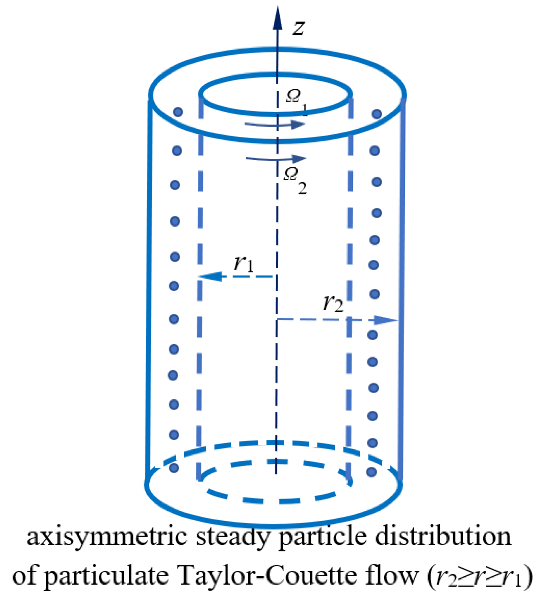
Let us consider the steady axisymmetric flow of an incompressible viscous fluid with axisymmetrically distributed particles between two infinitely long coaxial rotating cylinders, as shown in Figure 1. With the cylindrical coordinates (r, θ, z), the particle-fluid suspension occupies the space (r₁ ≤ r ≤ r₂, -∞ ≤ z ≤ +∞), and the inner and outer cylinders, of radii r₁ and r₂, rotate at two counter-clockwise angular velocities Ω₁ and Ω₂, respectively.

For the axisymmetric steady TC flow between two infinitely long cylinders in the cylindrical coordinates (r, θ, z), the flow is independent on (θ, z, t) and we seek for the solution with (u = w = 0, w_m = 0) and

$$\mathit{v}=\left(0,v\left(r\right),0\right),{\mathit{v}}_{\mathrm{m}}=\left(u_{\mathrm{m}}\left(r\right),v_{\mathrm{m}}\left(r\right),0\right),p\left(r\right),\delta \left(r\right).$$

(6)

where p(r) is the pressure field, (u, v, w) are the (r, θ, z) components of the velocity filed v of the suspension, while (u_m, v_m, w_m) are the (r, θ, z) components of the velocity field v_m of the mass center of representative unit cell, δ(r) is the particle volume fraction to be determined, and therefore the effective viscosity and mass density μ(r) and ρ(r) of the suspension which depend on δ(r) vary with the radial coordinate r. In particular, the volume-averaged radial velocity of the suspension $u=\delta u_{\mathrm{S}}+u_{\mathrm{f}}\left(1-\delta \right)=0$ implies that the radial flux $\delta u_{\mathrm{S}}$ of the particles is equal but opposite to the radial flux $\left(1-\delta \right)u_{\mathrm{f}}$ of the fluid and therefore the amplitude of radial velocity u_f of the fluid is vanishingly small as compared to the radial velocity u_S of the particles in the dilute limit (as δ is vanishingly small).

Note that

$$\nabla \mathit{v}{+\left(\nabla \mathit{v}\right)}^{\mathrm{T}}=\left[\begin{array}{ccc}0& \left(v_{,\mathrm{r}}-{\displaystyle \frac{v}{r}}\right)& 0\\ \left(v_{,\mathrm{r}}-{\displaystyle \frac{v}{r}}\right)& 0& 0\\ 0& 0& 0\end{array}\right],\nabla ·\left(\mu \left(r\right)\left[\nabla \mathit{v}+{\left(\nabla \mathit{v}\right)}^{\mathrm{T}}\right]\right)=\left[\begin{array}{c}0\\ \left({\displaystyle \frac{2}{r}}+{\displaystyle \frac{\partial }{\partial r}}\right)\left[\mu \left(r\right)\left(v_{,\mathrm{r}}-{\displaystyle \frac{v}{r}}\right)\right]\\ 0\end{array}\right].$$

(7)

It is verified that three of the eight Equations (1)–(4) are met identically by (6) and the other five give the following 5 nonlinear equations for (v, u_m, v_m, p, δ) as the functions of the variable r.

$$\rho \left[u_{\mathrm{m}}{\displaystyle \frac{\partial u_{\mathrm{m}}}{\partial r}}-{\displaystyle \frac{v_{\mathrm{m}}^2}{r}}\right]=-p_{,r},$$

(8)

$$u_{\mathrm{m}}{\displaystyle \frac{\partial \rho }{\partial r}}+\rho {\displaystyle \frac{1}{r}}{\left(r{u}_{\mathrm{m}}\right)}_{,r}=0,$$

(9)

$$\rho u_{\mathrm{m}}\left[{\displaystyle \frac{\partial v_{\mathrm{m}}}{\partial r}}+{\displaystyle \frac{v_{\mathrm{m}}}{r}}\right]=\left({\displaystyle \frac{2}{r}}+{\displaystyle \frac{\partial }{\partial r}}\right)\left[\mu \left(v_{,\mathrm{r}}-{\displaystyle \frac{v}{r}}\right)\right],$$

(10)

$$u_{\mathrm{m}}+a\left[u_{\mathrm{m}}{\displaystyle \frac{\partial u_{\mathrm{m}}}{\partial r}}-{\displaystyle \frac{v_{\mathrm{m}}^2}{r}}\right]=b\left({\displaystyle \frac{-v^2}{r}}\right),$$

(11)

$$v_{\mathrm{m}}+a\left[u_{\mathrm{m}}{\displaystyle \frac{\partial v_{\mathrm{m}}}{\partial r}}+{\displaystyle \frac{u_{\mathrm{m}}{v}_{\mathrm{m}}}{r}}\right]=v.$$

(12)

Kinematic boundary conditions on the normal velocity (based on the volume conservation of the particle-fluid suspension) and no-slip boundary conditions on two tangential velocities imposed on the velocity field v(x, t) of the suspension on the two rotating cylinders are met by (6) with

$${\left.v\right|}_{r=r_1}={\Omega }_1{r}_1,{\left.v\right|}_{r=r_2}={\Omega }_2{r}_2.$$

(13)

As shown below, all flow fields can be determined uniquely by Equations (1)–(4) with the above boundary conditions imposed on the velocity field v(x, t) of the suspension without additional boundary conditions on other velocity fields.

It should be stated that, instead of the above boundary conditions adopted by the present model, a different version of boundary conditions has been adopted in some two-fluid models of particle-laden fluids in Eulerian description. Specifically, the Saffman model [34] and its extended versions [35,36,37,38,39] have adopted the zero-velocity conditions (v_f = 0) of the velocity field v_f(x, t) of the carrier fluid (instead of the velocity field v(x, t) of the suspension) on fixed solid boundary. The two versions of the boundary conditions do not impose the zero-normal flux condition on the dispersed particles, and therefore the particle accumulation (suction) or invasion (injection) (with $\delta u_{\mathrm{S}}\ne 0$) on the solid boundary is allowed (see e.g., Michael and Norey [35] for TC flow with the Saffman model, where it is assumed that the particles can be deposited on the solid wall and the particles deposited on the solid wall can move into the TC system between the two cylinders). Particle accumulation/sedimentation on the solid boundaries could be a realistic physical phenomenon [5,35,40], although accurate description of particle accumulation on solid boundary requests extensive Lagrangian modeling of individual particles, which is beyond the scope of the two-fluid models in Eulerian description. On the other hand, if the zero-normal flux condition of particles is requested to be met on all sidewalls, the present model could be upgraded with a refined description of forces acting on dispersed particles (such as Faxen viscous force [5,22,32,41]), which adds higher-order terms to (A6), (A7), and (4) and makes it possible to impose additional zero-normal flux condition to the dispersed particles on solid boundary. It should be stated that this issue of the present model ($\delta u_{\mathrm{S}}\ne 0$ on the solid boundary, shared by the Saffman model and its many extended versions) does not appear in some important problems (such as stability of parallel plane or pipe flow, where the zero-normal velocity boundary condition of the carrier fluid or the suspension implies that the normal velocity of the particles vanishes on the solid boundary, see e.g., [34,39,42,43]), and particularly its influence on the flow field could be insignificant for a particle-laden fluid in the dilute limit.

Before our discussion on steady spatial distribution of particles, it is noted that exact solution of (9) gives $\left(r\rho u_{\mathrm{m}}\right)=\mathrm{c}\mathrm{o}\mathrm{n}\mathrm{s}\mathrm{t}\mathrm{a}\mathrm{n}\mathrm{t},$ and it follows from u = 0 and (A4) that $\rho u_{\mathrm{m}}=\left({\rho }_{\mathrm{S}}-{\rho }_{\mathrm{f}}\right)\delta u_{\mathrm{S}}$. Since the radial flux of the particles is equal but opposite to the radial flux of the fluid, u = 0 and u_m ≠ 0 can coexist for the non-neutrally buoyant particles $\left({\rho }_{\mathrm{S}}\ne {\rho }_{\mathrm{f}}\right)$ with the non-zero normal flux $\delta u_{\mathrm{S}}\ne 0$ of particles on the permeable solid walls [3,44,45,46,47,48,49]. Therefore, if the solid walls are impermeable and the zero-normal flux boundary condition $\delta u_{\mathrm{S}}=0$ of dispersed particles is imposed on the two cylinders, we shall have u_m ≡ 0 identically between the two cylinders. It is easily verified from (11) and (12) that u_m ≡ 0 implies that v = v_m and $\delta \left(r\right)\equiv 0$, and the non-trivial spatial distribution $\delta \left(r\right)\ne 0$ of particles cannot exist. It concludes that the non-trivial steady distribution of particles can exist only if $\delta u_{\mathrm{S}}\ne 0$ is allowed on the cylinders which means that the solid walls are permeable [3,44,45,46,47,48,49] and the particles and the fluid can be sucked or injected on the permeable cylinder walls with equal but opposite normal fluxes. The present paper is based on this assumption.

In what follows, we shall focus on Equations (9)–(12) for the three velocity fields and the particle distribution (v, u_m, v_m, δ), and the pressure p(r) can be determined from (8) once (u_m, v_m) are known. For a clear fluid (δ = 0) without dispersed particles, we have [1,2]

$$\delta =0:u_{\mathrm{m}}\left(r\right)=0,{v_{\mathrm{m}}\left(r\right)=v\left(r\right)=v}_0\left(r\right)=Ar+{\displaystyle \frac{B}{r}},$$

$$A={\displaystyle \frac{r_1^2{\Omega }_1-r_2^2{\Omega }_2}{r_1^2-r_2^2}},B={\displaystyle \frac{r_1^2{r}_2^2\left({\Omega }_2-{\Omega }_1\right)}{r_1^2-r_2^2}}.$$

(14)

Let us write the particle-disturbed flow fields as

$$v\left(r\right)=v_0\left(r\right)+v_1\left(r\right),u_{\mathrm{m}}\left(r\right)=u_{1m}\left(r\right),v_{\mathrm{m}}\left(r\right)=v_0\left(r\right)+v_{1\mathrm{m}}\left(r\right),\delta =\delta \left(r\right).$$

(15)

It follows from the boundary conditions (13) that

$${\left.v_1\right|}_{r=r_1}=0,{\left.v_1\right|}_{r=r_2}=0.$$

(16)

Here, let us focus on the dilute limit of particle-laden fluids when the volume fraction of particles is vanishingly small. Therefore, it is assumed that the disturbed velocity fields (v₁, u_1m, v_1m) due to dispersed particles are small as compared to the original flow field of a clear fluid without particles and the volume fraction δ(r) is much smaller than unity. With the Einstein formula $\mu ={\mu }_{\mathrm{f}}\left(1+2.5\delta \right)$, up to the first power of δ(r), the δ–dependent coefficients (μ, ρ, a, b) are expanded as:

$${\displaystyle \frac{\mu }{{\mu }_{\mathrm{f}}}}=1+2.5\delta \left(r\right),$$

$$\rho ={\rho }_{\mathrm{f}}\left[1+{\displaystyle \frac{\left({\rho }_{\mathrm{S}}-{\rho }_{\mathrm{f}}\right)}{{\rho }_{\mathrm{f}}}}\delta \left(r\right)\right],$$

$$a=a_0\left(1-\left[2.5-{\displaystyle \frac{\left({\rho }_{\mathrm{S}}-{\rho }_{\mathrm{f}}\right)}{{\rho }_{\mathrm{f}}+2{\rho }_{\mathrm{S}}}}\right]\delta \left(r\right)\right),a_0=\left(1+{\displaystyle \frac{{\rho }_{\mathrm{f}}}{{2\rho }_{\mathrm{S}}}}\right){\displaystyle \frac{2{\rho }_{\mathrm{S}}{r}_{\mathrm{S}}^2}{9{\mu }_{\mathrm{f}}}},$$

$$b=a_0\left[1-\left(\left[2.5-{\displaystyle \frac{\left({\rho }_{\mathrm{S}}-{\rho }_{\mathrm{f}}\right)}{{\rho }_{\mathrm{f}}+2{\rho }_{\mathrm{S}}}}\right]+2{\displaystyle \frac{{\left({\rho }_{\mathrm{S}}-{\rho }_{\mathrm{f}}\right)}^2}{{\rho }_{\mathrm{f}}\left({\rho }_{\mathrm{f}}+2{\rho }_{\mathrm{S}}\right)}}\right)\delta \left(r\right)\right].$$

(17)

Substituting (15) and (17) into (9)–(12) and ignoring all nonlinear terms of (v₁, u_1m, v_1m) and δ(r), the linear equations for (v₁, u_1m, v_1m) and $\delta \left(r\right)$ give

$${\left(r{u}_{1\mathrm{m}}\right)}_{,r}=0,$$

(18)

$$2A{\rho }_{\mathrm{f}}{u}_{1\mathrm{m}}={\mu }_{\mathrm{f}}\left({\displaystyle \frac{2}{r}}+{\displaystyle \frac{\partial }{\partial r}}\right)\left[\left(v_{1,\mathrm{r}}-{\displaystyle \frac{v_1}{r}}\right)\right]-5B{\mu }_{\mathrm{f}}\left({\displaystyle \frac{2}{r}}+{\displaystyle \frac{\partial }{\partial r}}\right)\left[{\displaystyle \frac{\delta \left(r\right)}{r^2}}\right],$$

(19)

$$u_{1\mathrm{m}}-{\displaystyle \frac{a_0}{r}}\left[2v_0{v}_{1\mathrm{m}}\right]=-{\displaystyle \frac{a_0}{r}}\left[2v_0{v}_1-\left(2{\displaystyle \frac{{\left({\rho }_{\mathrm{S}}-{\rho }_{\mathrm{f}}\right)}^2}{{\rho }_{\mathrm{f}}\left({\rho }_{\mathrm{f}}+2{\rho }_{\mathrm{S}}\right)}}\right)v_0^2\delta (r)\right],$$

(20)

$$v_{1\mathrm{m}}=v_1-2A{a}_0{u}_{1\mathrm{m}}.$$

(21)

And the pressure field p(r) can be determined from (8) once (u_m(r), v_m(r), and δ(r)) are known.

It is easily verified from (20) and (21) that if u_1m = 0, we have v₁ = v_1m and $\delta \left(r\right)=0.$ It is the case when r₁ = 0 (then (18) gives u_1m = 0). In what follows, let us consider TC flow with two cylinders r₁ > 0. Thus, (18) gives u_1m = X/r with a constant X (which represents the magnitude of the steady particle distribution, as shown below), and v₁(r) can be determined by two no-slip boundary conditions (16) and

$$u_{1\mathrm{m}}={\displaystyle \frac{X}{r}},\left({\displaystyle \frac{{\mathrm{d}}^2{v}_1}{\mathrm{d}{r}^2}}+{\displaystyle \frac{1}{r}}{\displaystyle \frac{\mathrm{d}{v}_1}{\mathrm{d}r}}-{\displaystyle \frac{v_1}{r^2}}\right)={\displaystyle \frac{{2AX\rho }_{\mathrm{f}}}{{r\mu }_{\mathrm{f}}}}+5B\left({\displaystyle \frac{2}{r}}+{\displaystyle \frac{\partial }{\partial r}}\right)\left[{\displaystyle \frac{\delta \left(r\right)}{r^2}}\right].$$

(22)

Explicit expression for δ(r) ≥ 0 in the dilute limit is determined from (20) and (21) by

$$u_{1\mathrm{m}}\left[1+4A{v}_0{\displaystyle \frac{a_0^2}{r}}\right]=\left(2{\displaystyle \frac{{\left({\rho }_{\mathrm{S}}-{\rho }_{\mathrm{f}}\right)}^2}{{\rho }_{\mathrm{f}}\left({\rho }_{\mathrm{f}}+2{\rho }_{\mathrm{S}}\right)}}\right)v_0^2{\displaystyle \frac{a_0}{r}}\delta (r).$$

(23)

Evidently, v₁m(r) can be determined from (21) once v₁(r) is determined. In particular, the expression for steady particle distribution given by (22) and (23) remains unchanged if the no-slip boundary conditions for the two tangential velocity components are imposed on the velocity field v_f of the carrier fluid (adopted by Saffman model and its extended versions) instead of the velocity field v of the suspension (assumed by the present model).

It is seen from (A4), (A8), and (22) that, up to the lowest-order approximation, the condition (∂δ/∂t = 0) for steady particle distribution is met by u_1m = X/r. Specifically, Equation (9) or its linearized version (18) ensures that, up to the lowest-order approximation, the volume fraction of particles at any location will not change with time, although the particle migration is not ceased due to the radial velocity field $u_{\mathrm{S}}\left(r\right)={\displaystyle \frac{\rho u_{1\mathrm{m}}\left(r\right)}{\delta \left(r\right)\left({\rho }_{\mathrm{S}}-{\rho }_{\mathrm{f}}\right)}}$ of dispersed particles. This explains why the coefficient X represents the magnitude of the steady particle distribution, and why such non-trivial steady spatial distribution does not exist when the inner cylinder is absent (X = 0). As stated previously, particle accumulation on solid boundary could be a realistic physical phenomenon [5,35,40], although a more accurate description requests numerical modeling in Lagrangian description of individual particles and usually beyond the scope of the two-fluid models in Eulerian description.

Clearly, the homogeneous Equation (22) has two independent solutions (r, 1/r), and an explicit particular solution of (22) can be obtained using the method of variation of parameters, as explained in [50]. For instance, for two co-rotating cylinders with Ω₁ = Ω₂ and B = 0, (22) has a particular solution $v_1^{*}\left(r\right)={\displaystyle \frac{{AX\rho }_{\mathrm{f}}}{{\mu }_{\mathrm{f}}}}\left[r\mathrm{l}\mathrm{n}r\right]$, and we have

$$B=0:v_1\left(r\right)={\displaystyle \frac{{AX\rho }_{\mathrm{f}}}{{\mu }_{\mathrm{f}}}}r\left[\mathrm{l}\mathrm{n}{\displaystyle \frac{r}{r_1}}+{\displaystyle \frac{r_2^2\mathrm{l}\mathrm{n}\frac{r_2}{r_1}}{\left(r_2^2-r_1^2\right)}}\left({\displaystyle \frac{r_1^2}{r^2}}-1\right)\right].$$

(24)

4. Discussions

TC flow causes particle migration and could possibly lead to a non-trivial steady axisymmetric spatial distribution of particles. Here, our interest focuses on the steady radial distribution δ(r) of particles determined by (23). In a recent study on TC flow with uniform distribution of particles without particle migration [50], it is shown that, up to the first-order solutions, the radial velocity u_S(r) of dispersed particles is determined by (with a₀ and v₀(r) defined in (14) and (17))

$$\mathrm{u}\mathrm{n}\mathrm{i}\mathrm{f}\mathrm{o}\mathrm{r}\mathrm{m}\delta :u_{\mathrm{S}}(r)=\left({\displaystyle \frac{\rho \left({\rho }_{\mathrm{S}}-{\rho }_{\mathrm{f}}\right)}{{\rho }_{\mathrm{f}}\left({\rho }_{\mathrm{f}}+2{\rho }_{\mathrm{S}}\right)}}\right){\displaystyle \frac{{2a}_0{v}_0^2\left(r\right)}{\left[r+{4A{a}_0^{2}v}_0\left(r\right)\right]}}.$$

(25)

Thus, the speed of u_S(r) is roughly dominated by the square of the mean azimuthal speed v₀(r) and its direction is determined by the signs of $\left({\rho }_{\mathrm{S}}-{\rho }_{\mathrm{f}}\right)$ and $\left[1+4A{v}_0{\displaystyle \frac{a_0^2}{r}}\right]$. Although Formula (25) is derived based on the assumption that particle migration is ignored and the volume fraction of particles is uniform, as seen below, it helps understand the final steady distribution of particles under the present assumption of dilute particulate flow.

It is noticed that, depending on the values of (r₁, r₂) and (Ω₁, Ω₂), $\left[1+4A{v}_0{\displaystyle \frac{a_0^2}{r}}\right]$ on left-hand side of (23) can change its sign (for instance, it is the case for examples 3 and 4 discussed below), and consequently u_1m(r) given by (22) has a discontinuity at the location determined by the root of $\left[1+4A{v}_0{\displaystyle \frac{a_0^2}{r}}\right]$ at which u_1m(r) changes its sign. Since steady spatial distribution of particles is determined by particle migration, and the latter is inactive when the particle Stokes number S_t (defined by the ratio of the Stokes relaxation time ${\displaystyle \frac{2{\rho }_{\mathrm{S}}{r}_{\mathrm{S}}^2}{9{\mu }_{\mathrm{f}}}}$ to the characteristic time of the flow, as shown in (29)) is much small or large than unity [50]. Therefore, we are particularly interested in the cases of Stokes number of the order of unity. As shown by (14), (17), and (29), Aa₀ scales with the Stokes number S_t of particles. Let us discuss the following four different cases of TC flow for the values of Aa₀ of the order of unity. It is seen from the definition that the size of particles determines the Stokes number which plays a key role in particulate flow.

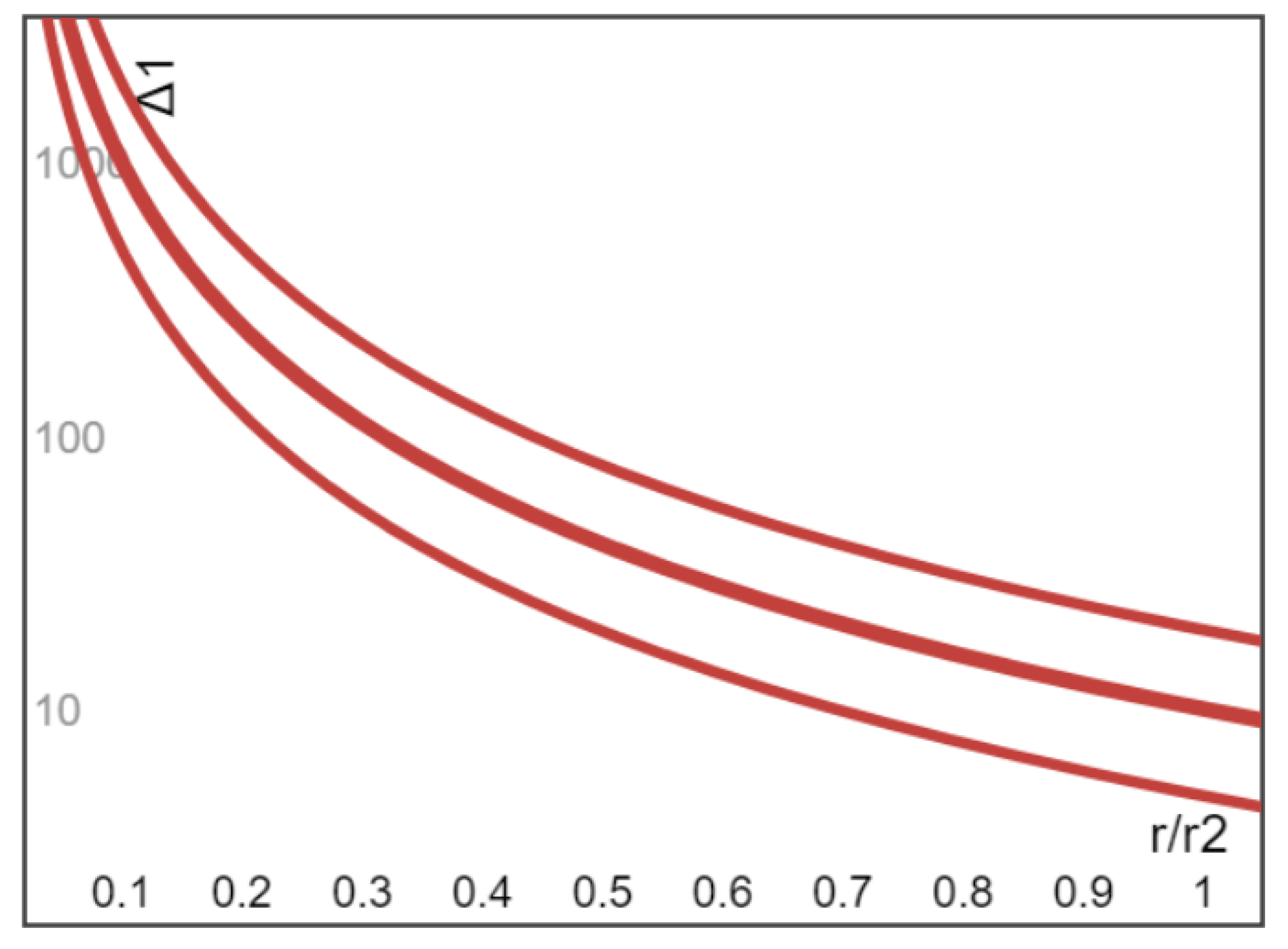
Example 1

(Ω₂ = Ω₁ > 0). Let us begin with the case of co-rotating cylinders (Ω₂ = Ω₁), thus it follows from (23) that the dimensionless particle distribution Δ₁(r) defined below with δ(r) ≥ 0 is given by

$$A={\Omega }_1,B=0,{\mathsf{\Delta }}_1\left(r\right)\equiv 2{\displaystyle \frac{{\left({\rho }_{\mathrm{S}}-{\rho }_{\mathrm{f}}\right)}^2}{{\rho }_{\mathrm{f}}\left({\rho }_{\mathrm{f}}+2{\rho }_{\mathrm{S}}\right)}}\left({\displaystyle \frac{A\delta \left(r\right)}{X}}{r}_2^2\right)={\displaystyle \frac{\left(1+4{\left(A{a}_0\right)}^2\right)}{\left({Aa}_0\right){\left(\frac{r}{r_2}\right)}^2}}.X>0.$$

(26)

The radial variation of Δ₁(r) vs (r/r₂) is plotted in Figure 2 for three values of Aa₀ = 0.1 (middle bold curve), 1.0 (lowest curve), and 5.0 (highest curve). Unlike a uniform distribution of particles [50], the non-uniformity of δ(r) has an effect on the rate of particle migration and leads to a non-uniform loss rate of the particles. As a result, the magnitude of the loss rate of particles for the co-rotating TC flow (Ω₂ = Ω₁) increases with azimuthal speed for increasing r, all particles moving to the outer cylinder are eventually deposited at r = r₂ and no longer remain inside the suspension, therefore final steady distribution δ(r) inside the suspension is a decreasing function of r. For example, it is seen from Figure 2 that when r₁ = 0.5r₂ with Aa₀ = 1, the particle volume fraction near the inner cylinder is a few times higher than the particle volume fraction near the outer cylinder.

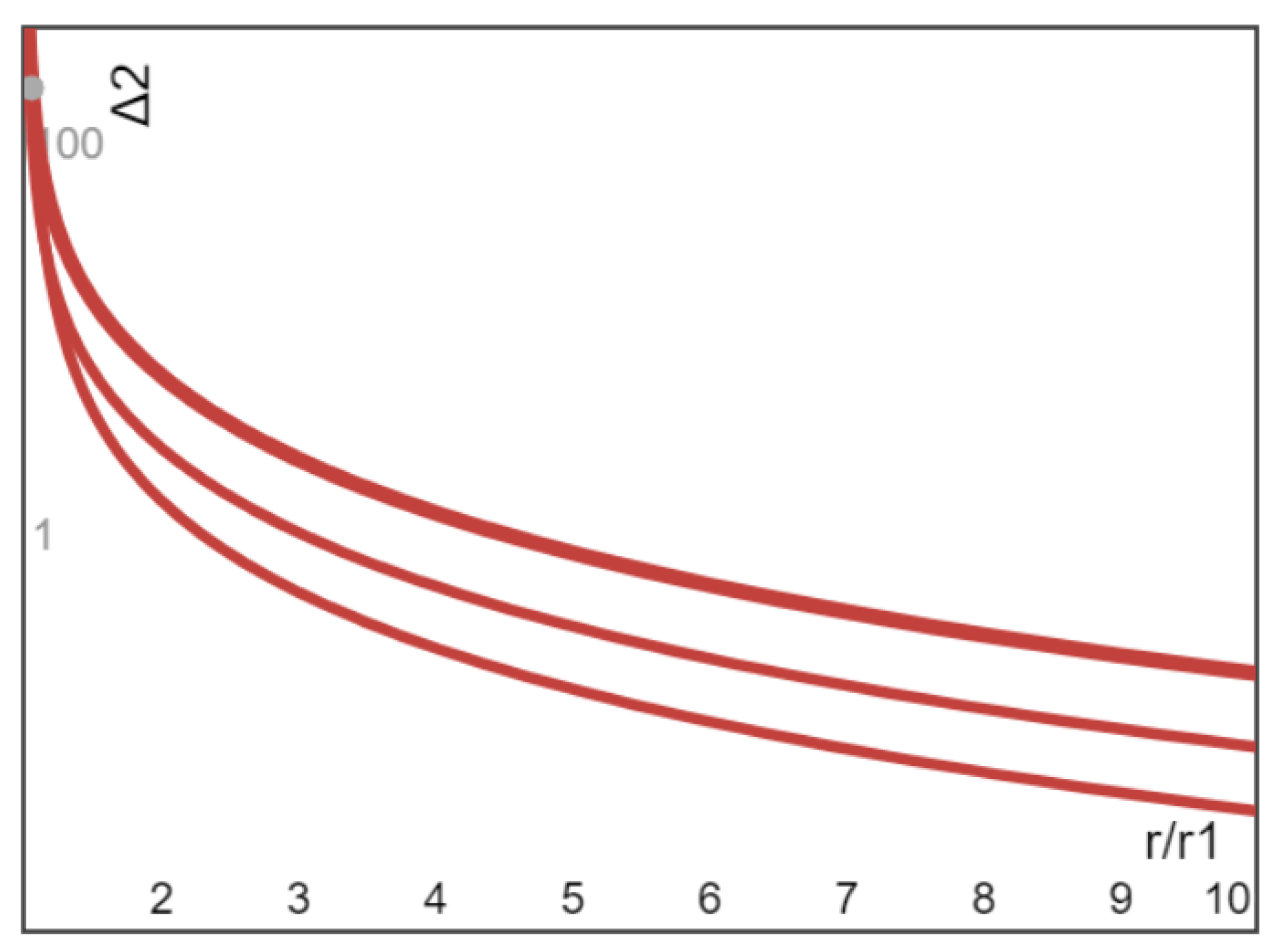
Example 2

(Ω₁ = 0, Ω₂ > 0). If the outer cylinder rotates with the inner cylinder fixed (Ω₁ = 0), we have the dimensionless particle distribution Δ₂(r) with δ(r) ≥ 0 given by

$$A={\displaystyle \frac{-r_2^2{\Omega }_2}{r_1^2-r_2^2}},B=-A{r}_1^2,{\Delta }_2\left(r\right)\equiv 2{\displaystyle \frac{{\left({\rho }_S-{\rho }_f\right)}^2}{{\rho }_f\left({\rho }_f+2{\rho }_S\right)}}\left({\displaystyle \frac{A\delta \left(r\right)}{X}}{r}_1^2\right)={\displaystyle \frac{\left(1+4{\left(A{a}_0\right)}^2\left[1-\left(\frac{r_1^2}{r^2}\right)\right]\right)}{\left({Aa}_0\right){\left(\frac{r}{r_1}\right)}^2{\left[1-\left(\frac{r_1^2}{r^2}\right)\right]}^2}},X>0.$$

(27)

The radial variation of Δ₂(r) for Example 2 (Ω₁ = 0) vs. (r/r₁) is plotted in Figure 3 for three values of Aa₀ = 0.5 (lowest curve), 2.0 (middle curve), and 5.0 (highest bold curve). Similar to Example 1 shown in Figure 2, because the loss rate of δ(r) monotonically increases with azimuthal speed for increasing r, from the fixed inner cylinder to the rotating outer cylinder, final steady distribution of particles inside the suspension is a decreasing function of r. For instance, it is seen from Figure 3 that when r₂ = 2r₁, the particle volume fraction near the fixed inner cylinder is about two orders of magnitude higher than the particle volume fraction near the rotating outer cylinder.

Examples 1 and 2 discussed above have $\left[1+4A{v}_0{\displaystyle \frac{a_0^2}{r}}\right]>0$ and therefore u_1m(r) given by (22) is smooth between the two cylinders with the same coefficient X for the entire domain. Now let us discuss two examples for which $\left[1+4A{v}_0{\displaystyle \frac{a_0^2}{r}}\right]$ can have a root r = r_c and change its sign at the location r = r_c.

Example 3

(Ω₂ = 0, Ω₁ > 0). For instance, for TC flow driven by rotating inner cylinder as the outer cylinder is fixed (Ω₂ = 0), an important case of particulate TC flow addressed in literature [5,6,11,22,23,25]. In this case, we have the dimensionless particle distribution Δ₃(r) with δ(r) ≥ 0 given by

$$A={\displaystyle \frac{r_1^2}{\left(r_1^2-r_2^2\right)}}{\Omega }_1,B=-A{r}_2^2,{Av}_0\left(r\right)=-r{A}^2\left[\left({\displaystyle \frac{r_2^2}{r^2}}\right)-1\right]<0,$$

$${\mathsf{\Delta }}_3\left(r\right)\equiv 2{\displaystyle \frac{{\left({\rho }_{\mathrm{S}}-{\rho }_{\mathrm{f}}\right)}^2}{{\rho }_{\mathrm{f}}\left({\rho }_{\mathrm{f}}+2{\rho }_{\mathrm{S}}\right)}}\left({\displaystyle \frac{-A\delta \left(r\right)}{X}}{r}_2^2\right)={\displaystyle \frac{\left(1+4{\left(A{a}_0\right)}^2\left[1-\left(\frac{r_2^2}{r^2}\right)\right]\right)}{\left(-{Aa}_0\right){\left(\frac{r}{r_2}\right)}^2{\left[\left(\frac{r_2^2}{r^2}\right)-1\right]}^2}},X>0\left(r>r_{\mathrm{c}}\right),X<0(r<r_{\mathrm{c}}).$$

(28)

The Stokes number S_t, the inner Reynolds number R_ei, and the S_t-(Aa₀) relation for this case are given by [25,43]

$$\begin{gathered} S_t=\left({\displaystyle \frac{{\rho }_{\mathrm{S}}}{{18\rho }_{\mathrm{f}}}}\right)\left({\displaystyle \frac{4r_{\mathrm{S}}^2}{{\left[r_2-r_1\right]}^2}}\right)R_{ei},R_{ei}=\left({\displaystyle \frac{r_1{\Omega }_1\left(r_2-r_1\right){\rho }_{\mathrm{f}}}{{\mu }_{\mathrm{f}}}}\right), \\ {S}_t={-a}_{0}A{\displaystyle \frac{\left(r_2+r_1\right)}{r_1}}. \end{gathered}$$

(29)

The radial variation of Δ₃(r) given by (28) vs. (r/r₂) is plotted in Figure 4 for four values of $\left|{Aa}_0\right|$ = 0.2, 0.5, 1.0, and 1.5. It is seen from Figure 4 that for relatively larger values of r/r₂, because the loss rate of δ(r) monotonically increases with azimuthal speed, unlike the Examples 1 and 2 for which azimuthal speed increases with r, the azimuthal speed for Example 3 (Ω₂ = 0) decreases with r and the loss rate of particles decreases with increasing r and attains its maximum at the rotating inner cylinder and its minimum at the fixed outer cylinder, and consequently final steady distribution of particles inside the suspension is an increasing function of r. For instance, it is seen from Figure 4 that it is the case when $\left|{Aa}_0\right|$ = 0.2 and r₁/r₂ > 0.3714 (which gives Stokes number S_t between 0.4 and 0.74), we have $\left[1+4A{v}_0{\displaystyle \frac{a_0^2}{r}}\right]>0$, the particle volume fraction near the fixed outer cylinder can be a few orders of magnitude higher than the particle volume fraction near the rotating inner cylinder. Similarly, when $\left|{Aa}_0\right|$ = 0.5 and r₁/r₂ > 0.7 (which gives Stokes number S_t between 1 and 1.2), we have $\left[1+4A{v}_0{\displaystyle \frac{a_0^2}{r}}\right]>0$ and the particle volume fraction near the fixed outer cylinder is a few orders of magnitude higher than the particle volume fraction near the rotating inner cylinder. This result for laminar TC flow is qualitatively consistent with the simulation results reported in [25] for turbulent TC flow with heavy particles driven by rotating inner cylinder with r₁/r₂ = 0.714 and initial value of ${\delta }_0=5.5\times {10}^{-5}$ (see Figure 6 of [25]), which indicate that when Stokes number S_t approaches unity (the maximum value of Stokes number studied in [25]), the particle concentration near the outer fixed cylinder is about two orders of magnitude larger than that in the main domain. Since the majority of existing related works have focused on preferential equilibrium position (rather than spatial distribution) of neutrally buoyant particles in channel or pipe flows, to the best of our current knowledge, more detailed comparison to known data of the present results on steady distribution of heavier or lighter particles cannot be made here due to the lack of available known data.

However, when the gap between two cylinders is large enough with sufficiently small radius ratio r₁/r₂, for sufficiently smaller values of r/r₂, Δ₃(r) given by (27) becomes negative and, as stated in the beginning of this section, u_1m(r) given by (22) has a discontinuity at the location r_c determined by the root of $\left[1+4A{v}_0{\displaystyle \frac{a_0^2}{r}}\right]$ at which the coefficient X of u_1m(r) changes its sign (see e.g., the location indicated by one black dot at r_c/r₂ ≈ 0.3714 in Figure 4 with Aa₀ = 0.2). In this case, all solutions of (18)–(21) should be given in two separated domains, r₁ ≤ r ≤ r_c and r₂ ≥ r ≥ r_c, respectively, although (22) remains valid for the two separate domains with two different values of the coefficient X of u_1m(r) of opposite signs. Thus, let us keep the coefficient X > 0 for the domain (r ≥ r_c) for larger r, then the coefficient X for u_1m(r) in the domain (r ≤ r_c) for small r is negative with an undetermined absolute value and the particle volume fraction δ(r) ≥ 0 given by (28) remains non-negative in the entire domain. This undetermined coefficient X for u_1m(r) in the domain (r ≤ r_c) and the total four coefficients of v₁(r) determined by (22) in the two separate domains will be determined by the three continuity conditions for azimuthal velocity v₁(r) and shear and normal stresses at r = r_c and the two no-slip boundary conditions (16) at the inner and outer cylinders. In this case, the steady distribution of particles varies non-monotonically in the radial direction with interior local maximum and/or minimum. A detailed mathematical solution is beyond the goal of the present work and is not explored here.

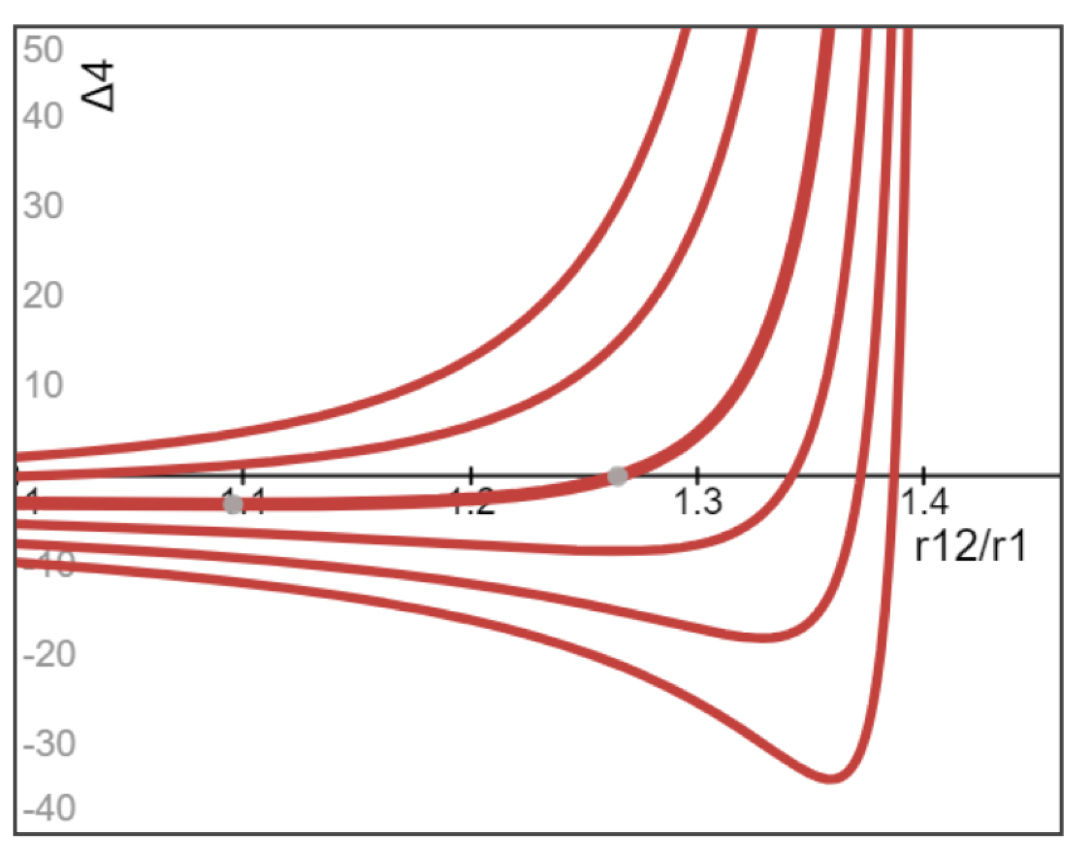
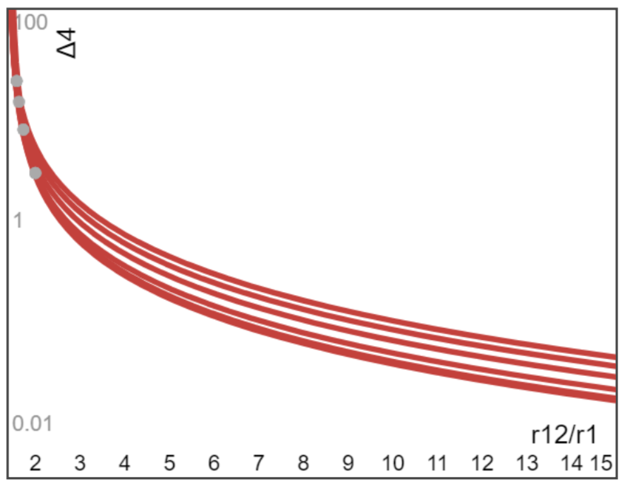
Example 4

(Ω₂ = −Ω₁). Finally, let us discuss the counter-rotating cylinders (Ω₁ = −Ω₂ > 0), thus we have the dimensionless particle distribution Δ₄(r) with δ(r) ≥ 0 given by

$$A=\left({\displaystyle \frac{r_1^2+r_2^2}{r_1^2-r_2^2}}\right){\Omega }_1,B=-2\left({\displaystyle \frac{r_1^2{r}_2^2}{r_1^2+r_2^2}}\right)A,v_0\left(r\right)=rA\left[1-2{\displaystyle \frac{r_1^2}{r_{12}^2}}\right],r_{12}\equiv r\sqrt{\left({\displaystyle \frac{r_1^2+r_2^2}{r_2^2}}\right)}>r_1,$$

$${\mathsf{\Delta }}_4\left(r\right)\equiv 2{\displaystyle \frac{{\left({\rho }_{\mathrm{S}}-{\rho }_{\mathrm{f}}\right)}^2}{{\rho }_{\mathrm{f}}\left({\rho }_{\mathrm{f}}+2{\rho }_{\mathrm{S}}\right)}}\left({\displaystyle \frac{{-A\delta }_1\left(r\right)}{X}}{r}_1^2\right)\left({\displaystyle \frac{r_2^2}{r_1^2+r_2^2}}\right)={\displaystyle \frac{\left(1+4{\left(A{a}_0\right)}^2\left[1-2\frac{r_1^2}{r_{12}^2}\right]\right)}{\left(-{Aa}_0\right){\left(\frac{r_{12}}{r_1}\right)}^2{\left[1-2\frac{r_1^2}{r_{12}^2}\right]}^2}},X>0\left(r>r_{\mathrm{c}}\right),X<0(r<r_{\mathrm{c}}).$$

(30)

It is seen from (30) that the mean azimuthal speed v₀(r) = 0 at (r₁₂/r₁) = √2 (the corresponding r is between r₁ and r₂), which indicates that, up to the leading-order approximation, the volume fraction of particles attains the maximum at this location determined by (r₁₂/r₁) = √2, as predicted by Δ₄(r) given in (30) and confirmed in Figure 5 and Figure 6. Therefore, we shall discuss the two cases (r₁₂/r₁) ≤ √2 and (r₁₂/r₁) ≥ √2, separately.

When $1\le \left({\displaystyle \frac{r_{12}}{r_1}}\right)\le \sqrt{2}$, r.h.s. of Δ₄(r) given in (30) is positive and monotonically increases with r for smaller values of (Aa₀), and becomes negative with its magnitude increasing with r for large S_t number, while r.h.s. of Δ₄(r) given in (30) for moderate values of (Aa₀) of the order unity varies non-monotonically with increasing r with interior local maximum/minimum. Actually, the radial variation of Δ₄(r) vs. (r₁₂/r₁) for the range $1\le \left({\displaystyle \frac{r_{12}}{r_1}}\right)\le \sqrt{2}$ is plotted in Figure 5 for six moderate values of Aa₀ = 0.3, 0.5, 1.0, 1.5, 2.0, and 2.5. It is seen from Figure 5 that, similar to Example 3 of rotating inner cylinder, because the loss rate of particle volume fraction decreases with increasing r and attains its maximum at the inner cylinder and its minimum at the outer cylinder, final particle distribution Δ₄(r) given in (30) inside the suspension is an increasing function of r. However, for sufficiently smaller values of r/r₂, Δ₄(r) given by (30) becomes negative and u_1m(r) given by (22) has a discontinuity at the location r_c determined by the root of $\left[1+4A{v}_0{\displaystyle \frac{a_0^2}{r}}\right]$ at which u_1m(r) changes its sign, see e.g., the location indicated by one grey dot between r₁₂/r₁ = 1.2 and 1.3 in Figure 5 on the bold curve with Aa₀ = 1.0. In such a case, all solutions of (18)–(21) should be given in two separated domains, r ≤ r_c and r ≥ r_c, respectively, although (22) remains valid for the two separate domains. Let us keep the coefficient X > 0 for the domain (r ≥ r_c) for larger r, then the coefficient X for u_1m(r) in the domain (r ≤ r_c) is negative with an undetermined absolute value and the particle volume fraction δ(r) ≥ 0 given by (30) remains non-negative in the entire domain. This undetermined coefficient X of u_1m(r) in the domain (r ≤ r_c) and the total four coefficients of v₁(r) in the two separate domains will be determined by the three continuity conditions for azimuthal velocity v₁(r) and shear and normal stresses at r = r_c and the two no-slip boundary conditions (16) at the inner and outer cylinders.

When $\left({\displaystyle \frac{r_{12}}{r_1}}\right)\ge \sqrt{2}$, on the other hand, r.h.s. of Δ₄(r) given in (30) is always positive and decreases with increasing r. The radial variation of Δ₄(r) vs. (r₁₂/r₁) is plotted in Figure 6 for five values of Aa₀ = 0.5, 1.0, 1.5, 2.0, and 2.5. It is seen from Figure 6 that, similar to Example 2 of rotating outer cylinder, because the loss rate of δ(r) monotonically increases with increasing r and attains its minimum at the inner cylinder and its maximum at the outer boundary, and final steady distribution inside the suspension is a decreasing function of r.

Here, some limitations of the present model should be highlighted. First, the present leading-order solutions based on the small parameter δ-expansion are limited to the dilute limit when the dimensionless particle distribution normalized by the coefficient X tends to zero as X tends to zero, which is intended to predict non-uniform spatial distribution of particles in the limit when the particle volume fraction becomes vanishingly small. In addition, as stated in the paper, all flow fields can be determined uniquely with the boundary conditions imposed on the velocity field of the suspension without additional boundary conditions on the velocity field of dispersed particles. As a result, the normal flux of dispersed particles does not necessarily vanish on solid boundary, which is equivalent to assume that the solid walls are permeable and the particles can be sucked or injected on the permeable cylinder walls [3,44,45,46,47,48,49]. In particular, the existence of non-trivial steady particle distribution predicted here depends on the assumed boundary condition ($\delta u_{\mathrm{S}}\ne 0$ allowed). Although particle accumulation on solid boundary can be a realistic physical phenomenon, its more accurate description requests extensive numerical modeling of individual particles in Lagrangian description and usually beyond the capability of the two-fluid models in Eulerian description. The influence of this limitation of the present model (shared by some other two-fluid models such as the Saffman model) on the accuracy of the present model near solid boundaries is to be clarified.

5. Conclusions

Steady spatial particle distribution of particulate TC flow with particles heavier or lighter than the carrier fluid is rarely studied in literature. In this work, a novel two-fluid model is used to study the radial steady distribution of non-neutrally buoyant particles in axisymmetric TC flow between two coaxial rotating cylinders in the dilute limit. An explicit expression for the radial distribution of particles of steady particulate TC flow is derived in the case when the solid walls are permeable, where the particles and the fluid can be sucked or injected with equal but opposite normal fluxes. In such a case, it is shown that:

(1)

The loss rate of particles due to particle migration is largely determined by the mean azimuthal speed, and the steady volume fraction of particles typically attains its maximum (or minimum) at the location of minimum (or maximum) azimuthal speed.

(2)

The steady distribution of particles is a monotonic function of the radial coordinate in some cases such as two co-rotating cylinders with equal angular velocity, or rotating outer cylinder with fixed inner cylinder.

(3)

In some other cases of wide-gap TC flow with a moderate value of particle Stokes number, such as counter-rotation of two cylinders with equal but opposite angular velocities or rotating inner cylinder with fixed outer cylinder, the steady particle volume fraction can vary non-monotonically in the radial direction with interior local maximum or/and minimum between the two cylinders.