A Numerical Investigation of Sinusoidal Flow in Porous Media with a Simple Cubic Beam Structure at 1 Hz and 100 Hz Under Different Porosity Conditions

Abstract

This study aims to clarify how porosity and frequency interact to influence permeability and flow behavior in porous media subjected to sinusoidal pressure variations. Specifically, we investigate oscillatory flow at 1 Hz and 100 Hz under varying porosity conditions using a pore-scale Computational Fluid Dynamics (CFD) model. The model is validated against the Johnson–Koplik–Dashen (JKD) model to ensure accuracy in capturing dynamic permeability. At 1 Hz, where the oscillation period greatly exceeds the system’s time constant $\tau$, the flow reaches a quasi-steady state with dynamic permeability approximating static permeability. Increasing porosity enhances Darcy velocity, with minimal phase difference between velocity and pressure. At 100 Hz, flow behavior depends on the ratio of the oscillation period $T$ to $\tau$. For high porosity ($\phi =0.840$, $T\approx \tau$), the flow does not fully develop before the pressure gradient reverses, leading to significant phase lag. For low porosity ($\phi =0.370$, $T\approx 12\tau$), the phase lag is smaller but remains non-zero due to the smooth temporal variation in pressure. This work contributes to the understanding of porous flow dynamics by revealing how porosity modulates both the amplitude and phase angle of dynamic permeability in frequency-dependent porous flows, providing a framework for predicting phase lag in frequency-sensitive applications.

1. Introduction

Fluid transport through porous media is widely studied due to its diverse applications in engineering [1,2,3,4,5], geophysics [6,7,8,9], and biological systems [10,11,12,13]. While steady-state flow in porous structures is well understood, oscillatory conditions introduce complex flow behaviors that deviate from classical theories [14,15]. At low frequencies, the flow behavior is primarily governed by geometric structure, where viscous effects dominate, and the system exhibits steady-state or quasi-steady flow behavior [16,17,18,19]. At high frequencies [20,21,22,23,24], the flow pattern is affected not only by the pore structure but also by the period of oscillation versus the step response time constant [20].

The behavior of porous flow under high- and low-frequency conditions involves key aspects such as wave propagation, pore geometry effects, non-linear flow dynamics, and acoustic properties. Soltani et al. [25], Morency and Tromp [26], and Benmorsli et al. [27] investigated wave propagation in porous media, utilizing Biot theory [14,15] to explore dispersion effects, attenuation mechanisms, and the influence of porosity on wave behavior. Cortis et al. [28] examined the fluid velocity in smooth and corrugated pore channels under high-frequency conditions, evaluated the classical JKD model [22] and developed modifications to the JKD model. Their findings refine high-frequency permeability modeling by addressing singularity effects in complex pore geometries. Langlois [29] investigated the high-frequency behavior of dynamic permeability in porous media with thin constrictions, including wedge-shaped pore geometries, and demonstrated that the Johnson et al. [22] high-frequency limit remains valid when accounting for a boundary layer comparable to the viscous skin depth. They further proposed a modified approximation to extend the model’s applicability to porous materials with complex microstructures. Champoux and Allard [30] extended the concept of characteristic length in dynamic tortuosity to describe the frequency dependence of the dynamic bulk modulus of the saturating fluids in porous media. Their theoretical predictions for high-frequency dynamic tortuosity and bulk modulus were validated through acoustic measurements, refining models for wave propagation in rigid-frame porous materials. Collectively, these studies provide a foundation for understanding porous flow behavior across different frequency regimes and highlight the role of geometry in shaping flow dynamics. Building on this, we examine how variations in porosity influence fluid flow under high- and low-frequency conditions.

In our previous study [20], we investigated the dynamic permeability versus the frequency of pressure gradient for a small porosity medium, $\phi =0.346$, with a body-centered cubic (BCC) sphere structure, and explored the physical mechanism associated with the dynamic permeability. The reduction in dynamic permeability is due to hindered flow development, which arises from alternating the sign of the pressure difference over a timescale close to the step response time constant. In addition, the phase angle of dynamic permeability is attributed to the rate of temporal variation in the pressure difference. Yet it is still unknown how the porosity affects the dynamic permeability and fluid flow phenomena.

Therefore, the objectives of this study are to investigate the influence of porosity on dynamic permeability and flow behavior in porous media under sinusoidal flow conditions at a low and a high frequency. A Computational Fluid Dynamics (CFD) model is used to solve the Navier–Stokes equation for the flow in pore scale. The model is validated against the JKD model, ensuring the accuracy in capturing dynamic permeability. The effects of porosity on the flow characteristics were investigated at 1 Hz and at 100 Hz by observing the dynamic permeability versus the porosity and the fluid flow visualization for porosities of 0.37 and 0.84. This study contributes to the field of fluid mechanics by advancing the understanding of sinusoidal flow in porous media and elucidating the effects of porosity and frequency on porous flow transport.

2. Mathematical Model

We used the Computational Fluid Dynamics (CFD) module in COMSOL Multiphysics 6.0 [31] to solve the Navier–Stokes equations for incompressible flow within a pore-scale fluid domain enclosed by solid walls. The governing equations are as follows:

$${\displaystyle \frac{\partial \rho }{\partial t}}+\nabla ·\left(\rho \mathit{V}\right)=0,$$

(1)

$${\displaystyle \frac{\partial }{\partial t}}\left(\rho \mathit{V}\right)+\nabla ·\left(\rho \mathit{V}\mathit{V}\right)=-\nabla p+\left\{\mu \left[\nabla \mathit{V}+{\left(\nabla \mathit{V}\right)}^T-{\displaystyle \frac{2}{3}}\left(\nabla ·\mathit{V}\right)\stackrel{=}{\mathit{I}}\right]\right\},$$

(2)

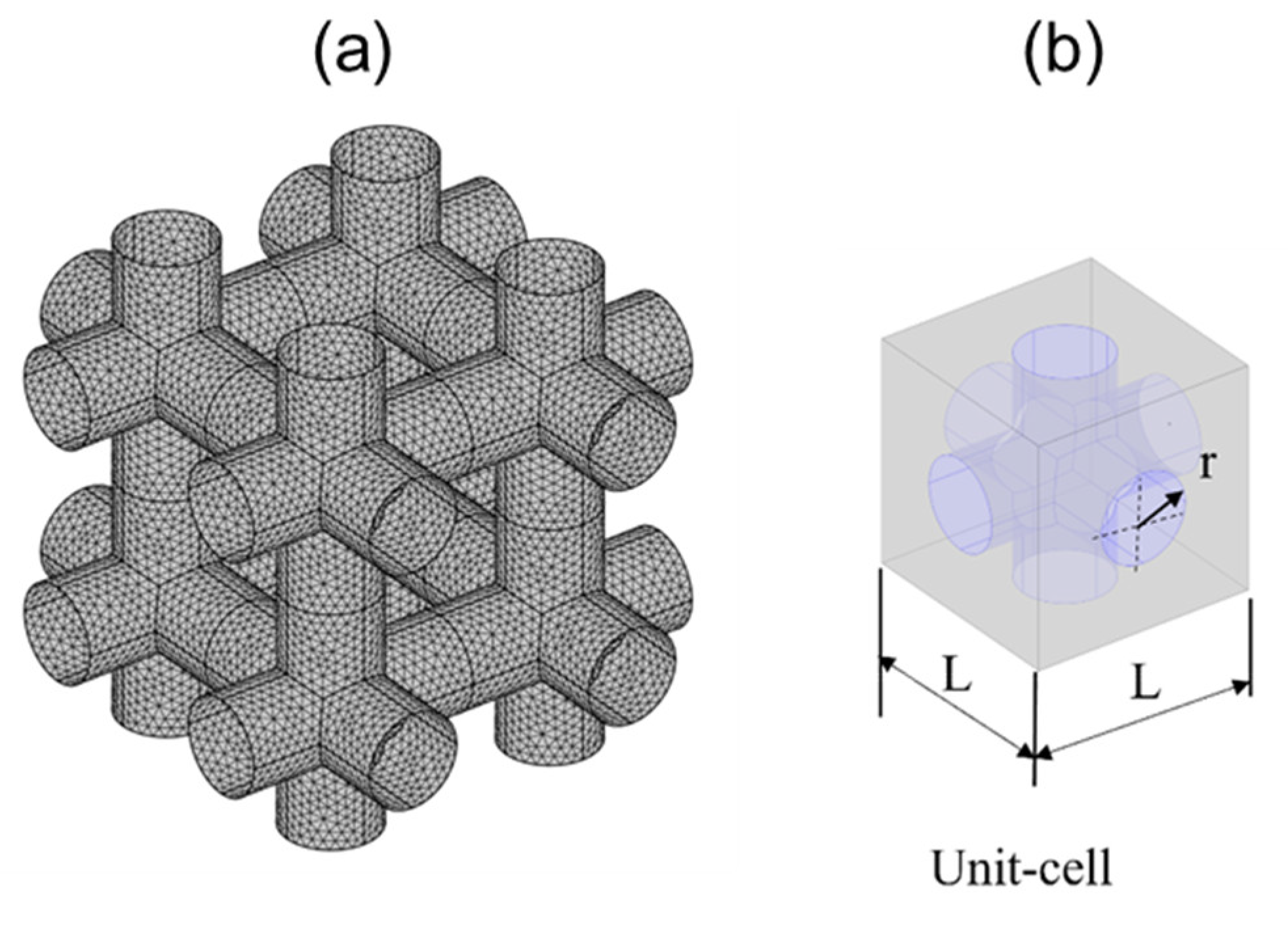
where $\mathit{V}=u \hat{i}+v \hat{j}+w \hat{k}$ is the fluid velocity, $\nabla p$ is the pressure gradient, $\rho$ is the density and $\mu$ is the dynamic viscosity. The porous medium is formed by a group of cylinders (beams) structured in a simple cubic (SC) lattice, as shown in Figure 1a. A fluid flows through the interconnected voids. To construct a microscopic model, we define a unit cell, illustrated in Figure 1b, and assume that the whole porous medium is simply multiple copies of this unit cell, geometrically and physically. The characteristic scales of this unit cell are the distance between two cylinders, L, and the radius of the cylinder, r.

Referring to Figure 2, the boundary conditions are as follows:

• Periodic boundary conditions are applied to the surfaces highlighted in purple, within which the velocity/pressure differences between the paired surfaces in the y-direction and in the z-direction are zero.
• No-slip conditions are imposed on the solid boundaries shown in blue.
• Periodic boundary conditions are enforced on the longitudinal sides of the unit cell—i.e., surfaces 1 and 2 marked in gray. These conditions ensure that a pressure difference can be applied across surfaces 1 and 2 while maintaining identical velocity values on both sides as follows:

$${\mathit{V}}_1={\mathit{V}}_2,$$

(3)

$$p_1-p_2=∆P \sin \left(2\pi ft\right).$$

(4)

In this study, Darcy’s law [16] is our primary study subject as follows:

$$U=-{\displaystyle \frac{\kappa }{\mu }}\nabla p.$$

(5)

Here, $U$ represents the Darcy velocity, which corresponds to the volumetric fluid velocity over the bulk volume of the porous medium. The parameter $\kappa$ denotes the permeability, which characterizes the influence of the porous structure. $-\nabla p=(P_1-P_2)/L$ is the negative pressure gradient. $P_{1, 2}$ are the average pressures at the void surfaces 1 and 2, respectively.

• Equation (5) can be expressed as follows:

$$\kappa ={\displaystyle \frac{\mu UL}{P_1-P_2}}.$$

(6)

$U$ and $P_{1,2}$ are calculated from the CFD results with,

$$U={\displaystyle \frac{1}{{\mathcal{V}}_f+{\mathcal{V}}_s}}{\int }_{{\mathsf{\Omega }}_f}u d\mathcal{V}={\displaystyle \frac{\phi }{{\mathcal{V}}_f}}{\int }_{{\mathsf{\Omega }}_f}u d\mathcal{V},$$

(7)

$$P_{1, 2}={\displaystyle \frac{1}{A_{1, 2}}}{\int }_{\partial {\mathsf{\Omega }}_{f1, 2}}{p}_{1, 2}d\mathcal{S}.$$

(8)

Here, $\phi ={\mathcal{V}}_f/({\mathcal{V}}_f+{\mathcal{V}}_s)$ denotes the porosity, where ${\mathcal{V}}_f$ is the fluid volume and ${\mathcal{V}}_s$ is the solid volume. ${\mathsf{\Omega }}_f$ represents the fluid domain, $\partial {\mathsf{\Omega }}_{f1}$ and $\partial {\mathsf{\Omega }}_{f2}$ are the void surfaces 1 and 2, respectively, and $A_1$ and $A_2$ are their corresponding cross-sectional areas.

Using the JKD model [22], we obtain [20] the following:

$$\kappa \left(\omega \right)={\displaystyle \frac{\mu \left|U\right|L e^{-i\omega t+i\theta }}{∆P e^{-i\omega t}}}={\displaystyle \frac{\mu \left|U\right|L{e}^{i\theta }}{\Delta P}}=\left|\kappa \left(\omega \right)\right|e^{i\theta }.$$

(9)

The parameters used in this study are summarized in

Table 1. Geometric and physical parameters.

Parameters	Value
$\mathrm{Reference} \mathrm{pressure} P_{ref}$/(Pa)	101,325
Cylinder radius r/(mm)	1
$\mathrm{Dynamic} \mathrm{viscosity} \mu$$/(\mathrm{Pa}·\mathrm{s}$)	$1.825\times {10}^{-5}$
$\mathrm{Density} \rho$/(kg/m3)	1.184
$\mathrm{Pressure} \mathrm{difference} ∆P$/(Pa)	1

. The working fluid is air at a temperature of 25 °C and a pressure of 1 atm. Note that in Table 1, the calculated porosity is 0.71. The fluid flow is identified as Stokes’ flow, as the difference in Darcy’s velocity between the solution of Equations (1) and (2) and that of Equations (1) and (2) with the inertial terms omitted is less than 0.1%.

3. Model Validation

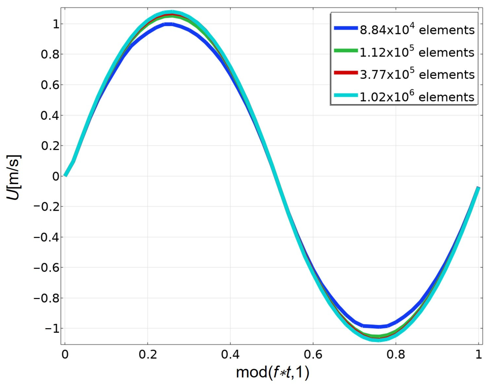
To validate mesh independence, we generated four different tetrahedral meshes with total element counts of $8.84\times {10}^4$, $1.12\times {10}^5$, $3.77\times {10}^5$, and $1.02\times {10}^6$. Figure 3 shows the Darcy velocities of 1 Hz for these four meshes, where $\mathrm{m}\mathrm{o}\mathrm{d}(f\times t,1)$ denotes the dimensionless time within an oscillation period. The maximum Darcy velocities are 0.99687, 1.0488, 1.064 and 1.0748 for the meshes with $8.84\times {10}^4$, $1.12\times {10}^5$, $3.77\times {10}^5$, and $1.02\times {10}^6$ elements, respectively. Selecting the densest mesh as reference, the relative differences associated with $U$ are 3.76%, 1.22%, and 0.50% for the three coarser meshes. Based on this comparison, we selected the mesh with $3.77\times {10}^5$ elements for the subsequent case studies.

To validate our simulation, we compared our dynamic permeability with that of the JKD model [22] as follows:

$${\kappa \left(\omega \right)}_{ \mathrm{J}\mathrm{K}\mathrm{D}}={\displaystyle \frac{{\kappa }_0}{\sqrt{1-\frac{4i{\alpha }_{\mathrm{\infty }}^2{\kappa }_0^2\rho \omega }{\mu L^2{\phi }^2}}-\frac{i{\alpha }_{\mathrm{\infty }}{\kappa }_0\rho \omega }{\mu \phi }}}.$$

(10)

Here, ${\kappa }_0$ is the static permeability, ${\kappa \left(\omega \right)}_{ JKD}$ is the dynamic permeability of JKD [22], ${\alpha }_{\infty }$ is the tortuosity, $\phi$ is the porosity, $L$ is a length scale, $\omega$ is the angular frequency, $\mu$ is the dynamic viscosity, and $\rho$ is the fluid density. The results shown in

Table 2. Dynamic permeability for the current model and the JKD model [22].

Frequency (Hz)	$\left|\mathit{\kappa }\left(\mathit{\omega }\right)\right|$ (m2)	$\left|{\mathit{\kappa }\left(\mathit{\omega }\right)}_{\mathbf{J}\mathbf{K}\mathbf{D}}\right|$ (m2)	Relative Difference
1	$2.39\times {10}^{-8}$	$2.36\times {10}^{-8}$	0.66%
10	$1.92\times {10}^{-8}$	$1.94\times {10}^{-8}$	0.71%
100	$6.88\times {10}^{-9}$	$6.78\times {10}^{-9}$	0.73%
1000	$2.18\times {10}^{-9}$	$2.22\times {10}^{-9}$	1.47%

and

Table 3. Phase difference for the current model and the JKD model [22].

Frequency (Hz)	$\mathit{\theta }$ (deg)	${\mathit{\theta }}_{\mathit{J}\mathit{K}\mathit{D}}$ (deg)	Relative Difference
1	1.58	1.57	0.32%
10	15.28	15.55	0.88%
100	68.23	70.07	1.33%
1000	85.17	87.21	1.18%

indicate that the maximum relative difference of $\left|\kappa \left(\omega \right)\right|$ between our model and the JKD model [22] is 1.47%, and the maximum relative difference of phase angle $\theta$ between our model and the JKD model [22] is 1.33%, respectively.

4. Results and Discussion

We varied L while keeping the cylinder radius r fixed to obtain seven different porosities: 0.84, 0.79, 0.71, 0.65, 0.59, 0.51, and 0.37. For each porosity, we consider a low frequency of 1 Hz and a high frequency of 100 Hz. Note that the low and high frequencies can be judged based on the Womersley number [32]. The Womersley number ($W_o$) is a dimensionless parameter that characterizes oscillatory flow, where $W_o^2$ represents the ratio of oscillatory inertial force to the viscous force as follows:

$$W_o^2={\displaystyle \frac{r^2\omega \rho }{\mu }}.$$

(11)

When $W_o\ll 1$, the oscillatory inertial force is insignificant as compared to the viscous force, corresponding to the low-frequency flow. While $W_o\gg 1$, the oscillatory inertial force is much larger than the viscous force, corresponding to the high-frequency flow. Substituting 1 Hz and 100 Hz into Equation (11) yields values of 0.63 and 6.34, respectively. We claim that 100 Hz is a high frequency and 1 Hz a low frequency. This classification is justified by observing Figures 5–8, which will be discussed later.

In Figure 4, we present the Darcy velocity for different porosities. The vertical axis represents Darcy’s velocity, while the horizontal axis denotes the dimensionless time. For the cases at 1 Hz, Figure 4a shows that the porosity significantly influences the Darcy velocity. The maximum $U$ increases with the porosity, while the phase differences between $U$ and $P_1-P_2$ are relatively small for all cases. High-porosity structures (0.84 and 0.79) exhibit greater velocity response amplitudes, indicating reduced flow resistance and enhanced fluid mobility. In contrast, the low-porosity structure (0.37) has substantially lower Darcy velocity due to the high surface resistance resulting from the more compact configuration. For 100 Hz, Figure 4b shows that the porosity significantly influences the Darcy velocity. The maximum $U$ increases with the porosity, while the phase differences between $U$ and $P_1-P_2$ become larger as porosity increases. The low-porosity structure (0.37) exhibits minimal velocity fluctuations and relatively smaller phase differences.

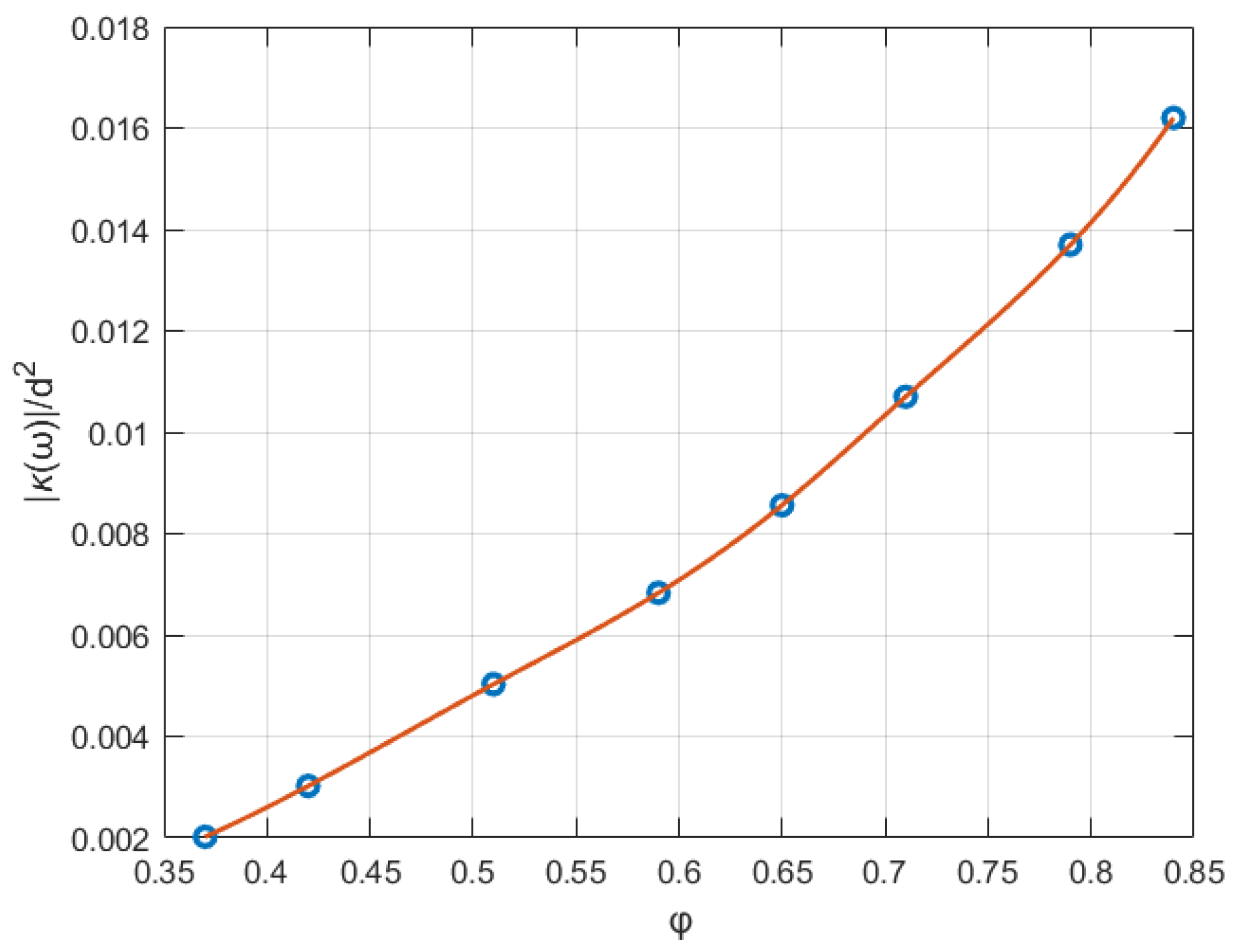
The effect of porosity on dynamic permeability with $f=1 \mathrm{Hz}$ is shown in Figure 5 for the amplitude $\left|\kappa \left(\omega \right)\right|/d^2$ and Figure 6 for the phase angle $\theta$ of $\kappa \left(\omega \right)$. Note that $\left|\kappa \left(\omega \right)\right|/d^2$ is based on the dimensionless analysis proposed in [22], where $d$ is the diameter of the SC beam. 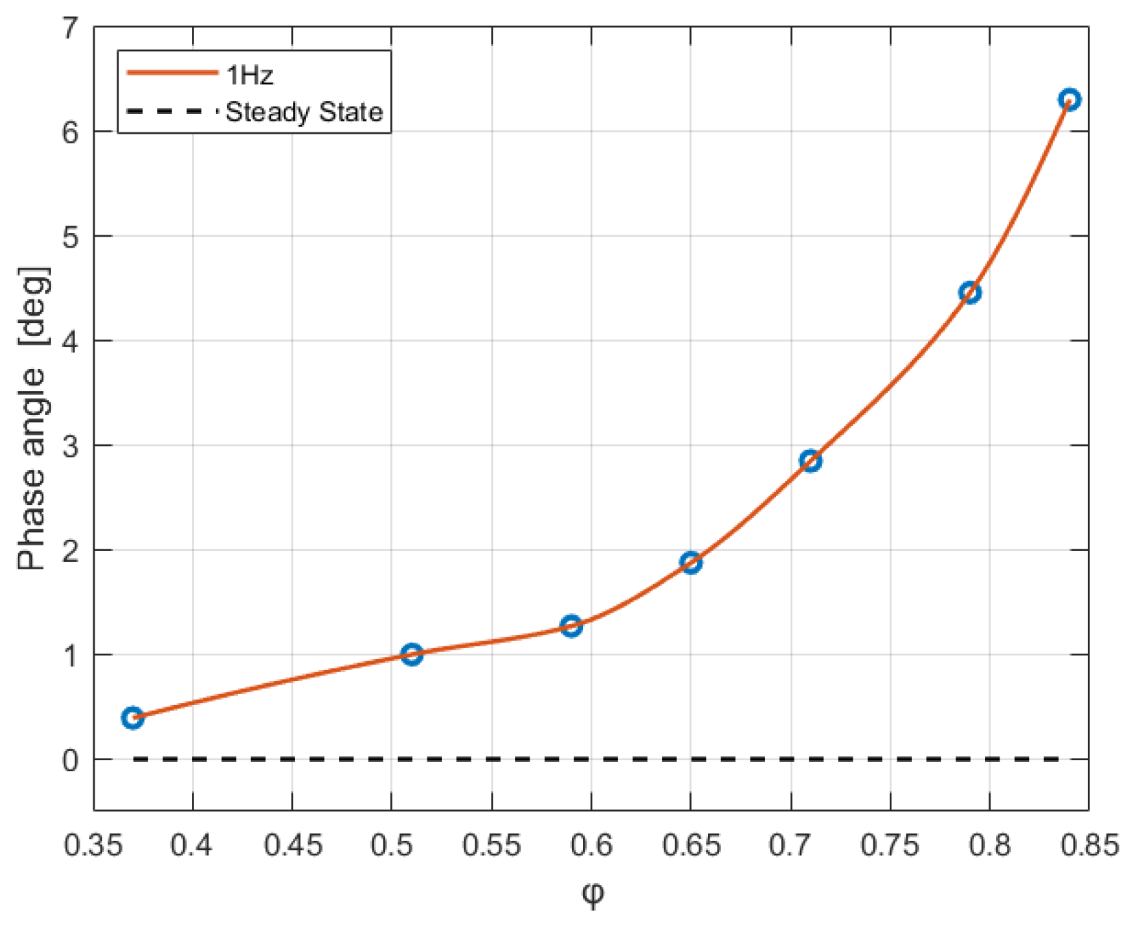In Figure 5, $\left|\kappa \left(\omega \right)\right|/d^2$ increases significantly with porosity, with its maximum and minimum values differing by nearly tenfold. In addition, the dashed line representing steady-state flow coincides with the solid line for the 1 Hz flow, indicating that the 1 Hz condition closely approximates steady flow. In Figure 6, the phase angle $\theta$ is small, which is consistent with observation of the phase difference between $U$ and $P_1-P_2$ shown in Figure 4a. The near-zero phase angle shows that the imaginary part of $\kappa \left(\omega \right)$ is negligible, indicating that the 1 Hz condition is in the low-frequency regime, i.e., $W_o\ll 1$. $\left|\kappa \left(\omega \right)\right|/d^2$ rises nearly tenfold for porosity increasing from 0.37 to 0.84 with a sharper increase at higher porosities, suggesting enhanced fluid transport capacity.

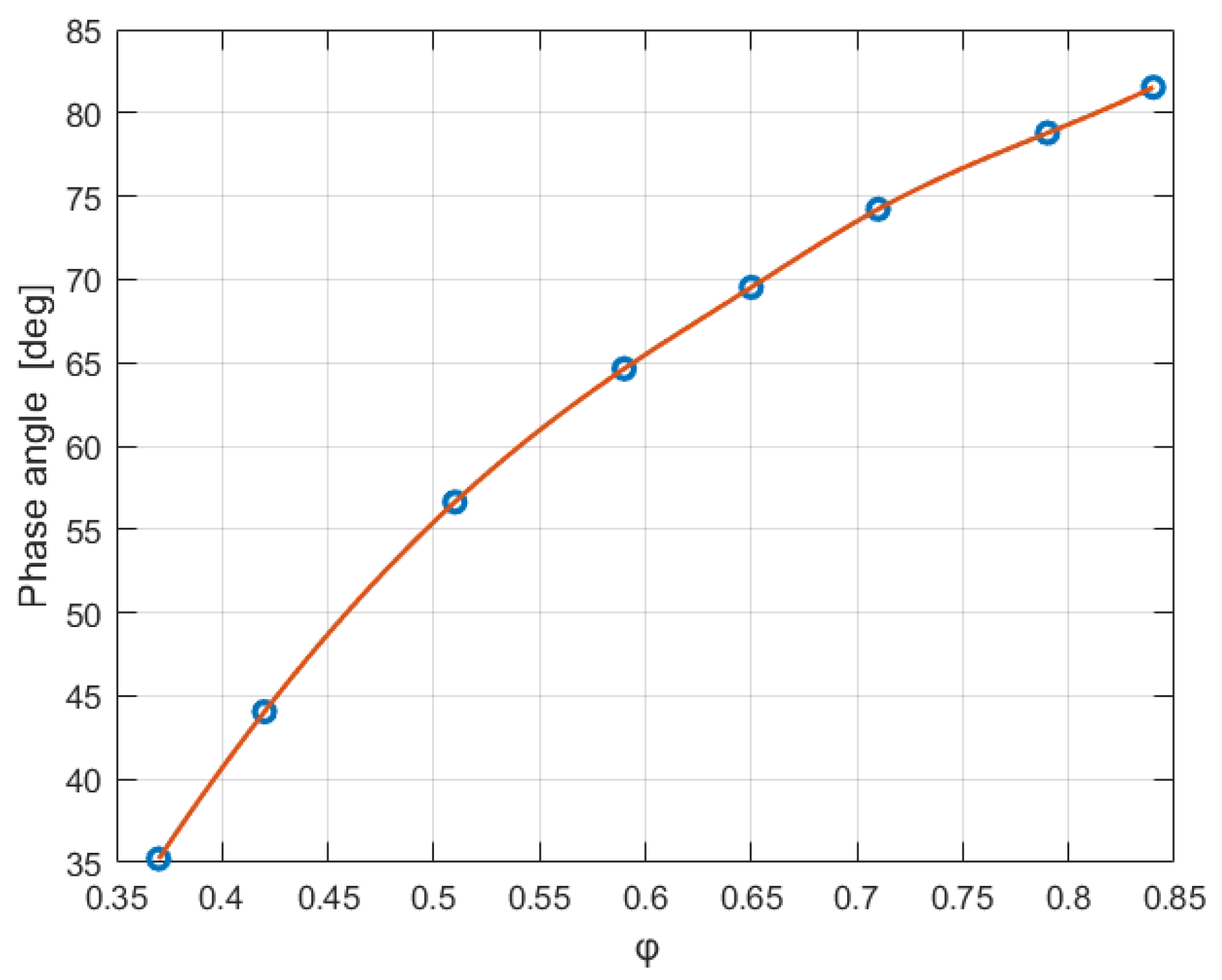
The effect of porosity on dynamic permeability at $f=100 \mathrm{H}\mathrm{z}$ is shown in Figure 7 and Figure 8. In Figure 7, $\left|\kappa \left(\omega \right)\right|/d^2$ increases with porosity, with the maximum and minimum values differing by nearly ninefold. In Figure 8, the phase angle $\theta$ increases with porosity, varying from 35° to approximately 80° when porosity increases from 0.37 to 0.84. As the non-zero phase angle is equivalent to the non-zero imaginary part, the 100 Hz condition is in the high-frequency regime, i.e., $W_o\gg 1$.

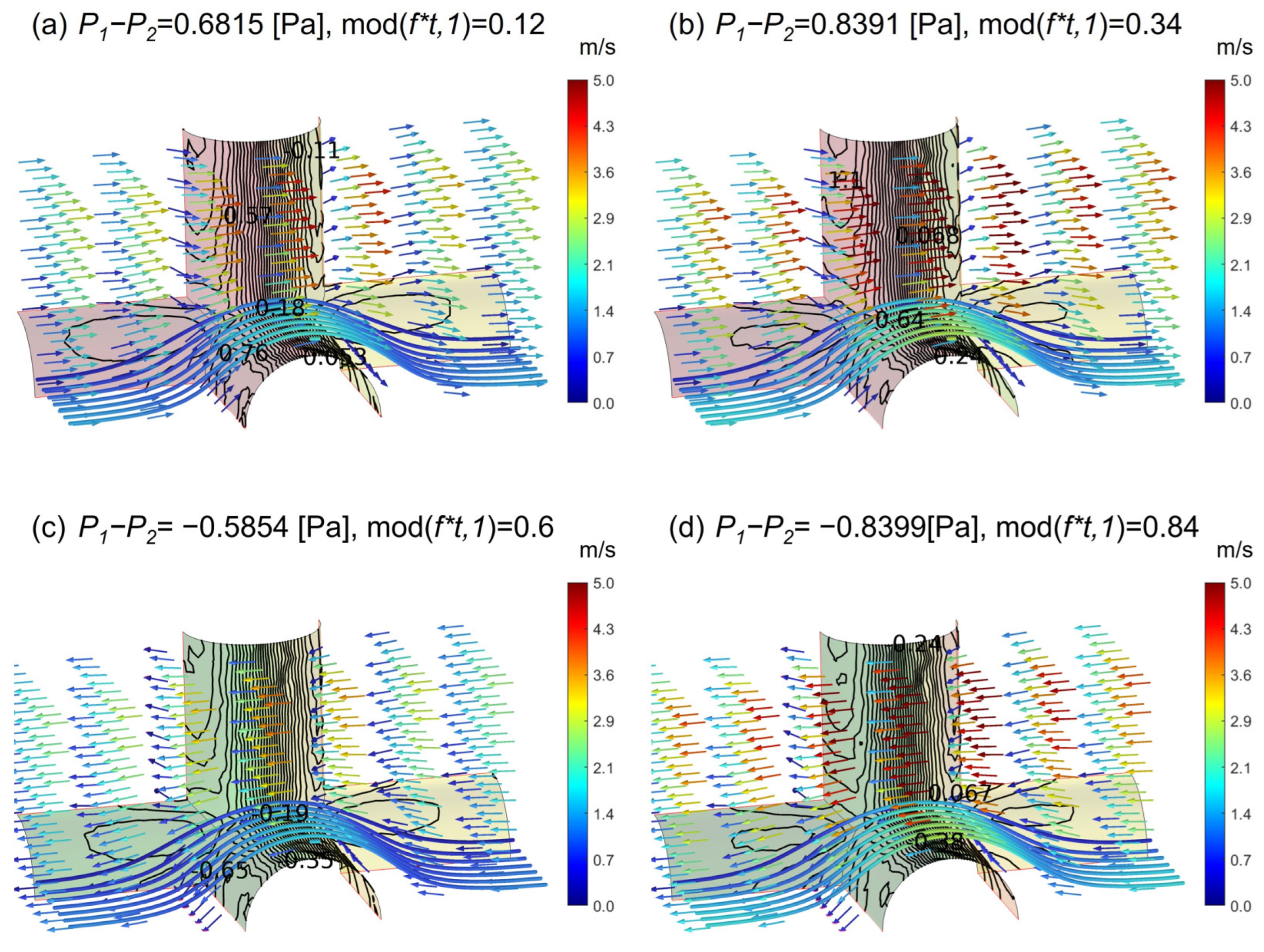
We further examine the fluid flow field for the case with porosity 0.84, where the maximum phase difference occurs, as in Figure 8. Figure 9 and Figure 10 show the flow fields at 1 Hz and 100 Hz, respectively. Each subfigure shows the pressure contour on wall surfaces and the normalized velocity vector $\mathit{V}/\left|\mathit{V}\right|$, in which the velocity magnitude is presented by color. The pressure distribution on the wall is also shown using a color scale ranging from $-0.6 \mathrm{Pa}$ to $0.6 \mathrm{Pa}$. The color transitions from red to yellow for values between 0.6 Pa and $0 \mathrm{P}\mathrm{a}$, and from yellow to green for values between $0 \mathrm{P}\mathrm{a}$ and $-0.6 \mathrm{P}\mathrm{a}$. In Figure 9a–d, corresponding to the 1 Hz condition, the flow field direction aligns with the negative direction of the pressure gradient, indicating a nearly synchronous response. In contrast, Figure 10a,c, under the 100 Hz condition, shows that the flow direction is opposite to the negative direction of the pressure gradient, clearly demonstrating the phase difference phenomenon at high frequency.

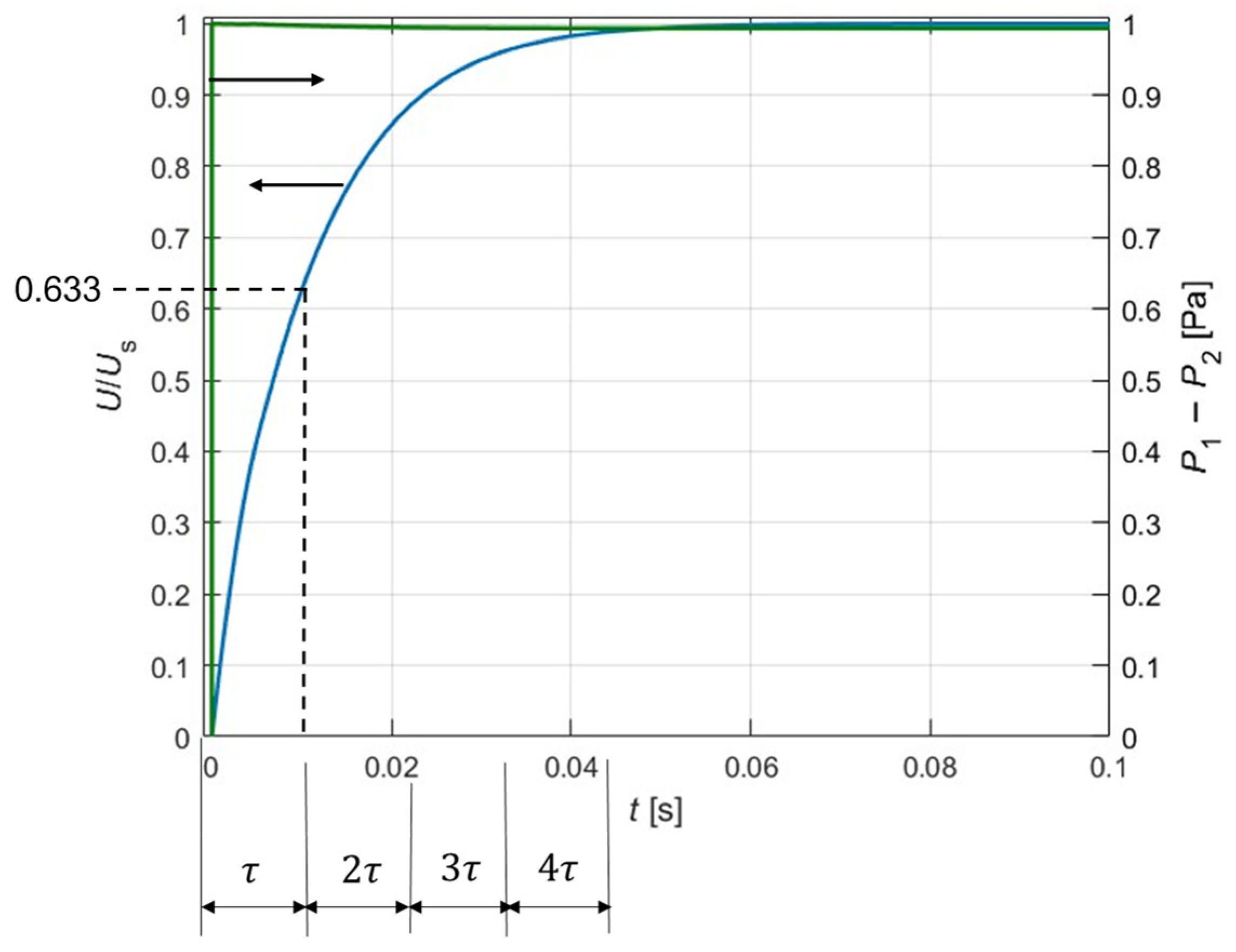
From our previous study [20], we found that the significant difference in velocity field behavior between low and high frequencies, as well as the increasing phase angle of $\kappa \left(\omega \right)$ with frequency, is closely related to the relationship between the oscillation time period and the flow system’s step response time constant. Note that fluid flow requires time to fully respond to a change in the pressure field. Therefore, at high frequencies, it is plausible that the flow may not fully respond to the applied pressure gradient before the gradient reverses direction. To estimate the time required for the flow to respond to a pressure field, we considered a step response flow described as follows:

$$P_1-P_2=∆PH\left(t\right).$$

(12)

$H\left(t\right)$ is the heavy-side function, defined as $H=0$ when $t<0$ and $H=1$ when $t\ge 0$. As shown Figure 11, the Darcy velocity, the response signal, can be expressed as follows:

$$U\left(t\right)=U_s\left(1-e^{-{\displaystyle \frac{t}{\tau }}}\right),$$

(13)

where $\tau$ is a time constant and $U_s$ is the steady-state Darcy velocity. The value of $\tau$ can be obtained by finding the time at which $U/U_s=0.633$. Figure 11 also shows that when $t=4\tau$, $U\approx U_s$, indicating that a steady-state flow has been reached.

Table 4. Time constant for different porosities.

Lattice Structure	$\mathbf{Porosity} \mathit{\phi }$	$\mathbf{Step} \mathbf{Response} \mathbf{Time} \mathbf{Constant} \mathit{\tau }$(s)
SC beam	0.840	$9.26{ \text{×} 10}^{-3}$
	0.370	$8.49{ \text{×} 10}^{-4}$
BCC sphere [20]	0.346	$9.60 {\text{×} 10}^{-4}$

lists the time constants $\tau$ for $\phi =0.840$ and $0.370$ in our SC beam structure and $\phi =0.346$ in the BCC sphere structure from the previous study [20]. It is found that in our current study, the SC beam structure, $\tau =9.26{ \text{×} 10}^{-3} \mathrm{s} \approx 10 \mathrm{ms}$ for $\phi =0.840$, and $\tau =8.49{ \text{×} 10}^{-4} \mathrm{s} \approx 0.85 \mathrm{ms}$ for $\phi =0.370$. For the BCC sphere structure, $\tau =9.60{ \text{×} 10}^{-4} \mathrm{s} \approx 1 \mathrm{ms}$ for $\phi =0.346$. It is interesting to note that despite the structural differences, the time constants for the lower porosities of 0.370 and 0.346 remain relatively similar—approximately 0.85 ms and 1 ms, respectively. At a frequency of 1 Hz, the oscillation time period $T=1 \mathrm{s}$ is much larger than $\tau$ for all three porosities. According to Figure 11, it takes approximately $4\tau$ for the flow to fully respond to a step-function input. Therefore, the fluid has sufficient time to fully develop, and the flow can be considered quasi-steady under 1 Hz conditions. At a high frequency of 100 Hz, the oscillation time period $T=10 \mathrm{ms}$. For $\phi =0.840$, $T\approx \tau$. In this case, the fluid flow does not have enough time to fully develop before the applied pressure gradient reverses, resulting in a significant phase difference between the velocity and the pressure gradient. For $\phi =0.370$, $T\approx 12\tau$. Therefore, the phase difference between the velocity and the pressure gradient is expected to be smaller than that observed for $\phi =0.840$. In our case, the phase difference is approximately ${35}^{\mathrm{o}}$ for $\phi =0.370$ and ${81}^{\mathrm{o}}$ for $\phi =0.840$. It should be noted that the above discussion does not account for the temporal variation in the sinusoidal pressure difference, in which the pressure varies smoothly with time. Our previous study [20] showed that the phase angle of dynamic permeability, as well as the phase difference between $U$ and $P_1-P_2$, arises from the rate of change of $P_1-P_2$. Therefore, even when $T\approx 12\tau$, the phase angle may remain non-zero.

5. Conclusions

This study investigates the impact of porosity on fluid flow under low-frequency (1 Hz) and high-frequency (100 Hz) conditions, revealing the coupling mechanism between porosity and frequency. A pore-scale computational model was employed to solve the Navier–Stokes equations, and the simulation results were validated against the JKD model [22], confirming the model’s accuracy in capturing the dynamic permeability values.

At a frequency of 1 Hz, the flow is in a quasi-steady state, the permeability equals the static permeability, and velocity oscillations are minimal. In addition, the Darcy velocity increases with porosity, and the phase difference between the Darcy velocity and the applied pressure difference is nearly zero, resulting in a near-zero phase angle of dynamic permeability.

At a frequency of 100 Hz, the Darcy velocity also increases with porosity, but the phase difference between the Darcy velocity and the applied pressure difference becomes significant. At a porosity of 0.84, the velocity direction is opposite to the negative pressure gradient at the dimensionless times of 0.12 and 0.6.

Our study reveals that despite structural differences, porous media with smaller porosities ($\phi =0.370$ and $\phi =0.346$) exhibit similar step response time scales. At 1 Hz, where the oscillation period ($T=1 \mathrm{s}$) is much larger than the time constant $\tau$, the flow has sufficient time to fully develop, resulting in a quasi-steady state. At 100 Hz, the flow response varies with porosity. For $\phi =0.840$, where $T\approx \tau$, the flow does not fully develop before the pressure gradient reverses, leading to a significant phase difference between the velocity and the pressure difference. For $\phi =0.370$, where $T\approx 12\tau$, the phase difference is smaller (35°), but remains non-zero due to the temporal variation in the pressure difference.

These findings highlight the fundamental mechanisms governing porous flow behavior under different frequency regimes, offering valuable insights for porous flow applications. Future studies could include parametric studies involving more complex pore geometries and a broader span of frequencies.