Abstract
Turbulent flows over a semi-circular cylinder (a limiting case of a thick airfoil with a chord equal to the diameter base) are investigated using high-fidelity large-eddy simulations at a diameter-based Reynolds number, Re = 130,000, Mach number, M = 0.05, and a zero angle of attack. The aerodynamic flow control system, designed with two trapped vortex cells, achieves a complete non-separated flow over the bluff body, except for low-scale turbulence effects, reaching approximately 80% of the theoretical lift coefficient limit ( for the half-circular airfoil). Viscous effects are analyzed using the conventional Reynolds-averaged Navier–Stokes approach for a broad range of Reynolds numbers, 75,000 ≤ Re ≤ 1,000,000. Numerical results demonstrate that the aerodynamic properties of the implemented concept are independent of the Reynolds number within this interval, highlighting its significant potential for further development.
1. Introduction
Aerodynamic flow control (AFC) is a multi-disciplinary area of research and development that holds the potential to revolutionize the design and performance of various aerodynamic systems. AFC focuses on manipulating and controlling the flow of air over an object’s surface to improve its aerodynamic performance like to reduce drag, enhance lift, and improve the overall efficiency and stability of the object, which is often an aircraft, but can also include cars, wind turbines, and other aerodynamic structures like buildings and bridges.
There are various techniques used in aerodynamic flow control, including passive, active, and hybrid [1]. Passive flow control involves typically designing the object’s surface in a way that naturally influences airflow like vortex generators, winglets, and riblets, which are small surface features that help manage airflow and reduce drag. Active flow control uses external devices or systems to manipulate airflow dynamically like blowing or suction, where air is either injected into or removed from the boundary layer to delay separation and reduce drag. Other techniques are synthetic jets, plasma actuators, and electromagnetic fields. The hybrid flow control method combines both passive and active techniques and tries to maximize the benefits of both approaches. This method often involves the use of passive devices in conjunction with active systems to achieve optimal aerodynamic performance.
The development and implementation of AFC technologies have significant implications for various industries. In aviation, these technologies can lead to more fuel-efficient and environmentally friendly aircraft by reducing drag and enhancing lift. In the automotive industry, aerodynamic flow control can improve vehicle performance and fuel efficiency. Additionally, in renewable energy, optimizing airflow over wind turbine blades can increase energy production. Another critical area in hydro- and aerodynamics is the control of bluff body wakes and the suppression of the related vortex shedding, which allows us to significantly reduce unsteady loads and induced vibrations.
Recent literature surveys have highlighted that AFC systems and methods have become a significant trend across various industrial sectors. Several noteworthy papers have been identified in this context as follows: Greenblatt and Williams [2] and Lee et al. [3] presented state-of-the-art methods for the aviation industry; Bharghava et al. [4] provided a comprehensive survey of synthetic jet applications for active flow control systems; Mariaprakasam et al. [5] discussed methods for reducing aerodynamic drag in vehicles; Rashidi et al. [6] offered a detailed review of technologies for vortex-shedding suppression and wake-dynamics control; Chen et al. [7] presented results dedicated to the flow control for circular cylinders; Derakhshandeh and Alam [8] and Lekkala et al. [9] reviewed the wakes of bluff bodies; Tayebi and Torabi [10] analyzed flow control techniques for vertical wind turbines.
In the aerospace industry, one example of an innovative project is the CRANE (control of revolutionary aircraft with novel effectors) program. The goal of this strategic initiative is to design, build, and flight test a new X-plane that incorporates AFC as a core design feature. The experimental aircraft, now designated as the X-65, is being developed for the Defense Advanced Research Projects Agency CRANE program [11]. The X-65 is designed to demonstrate and test the use of AFC to control flight at tactical speeds and improve performance throughout the flight envelope, and it has potential for both commercial and military applications. AFC technology replaces traditional flaps and rudders with actuators and effectors to control airflow, resulting in improved aerodynamics, reduced weight, and mechanical simplicity. The aerodynamic community believes that AFC-based flight control systems will be smaller and lighter than conventional systems, providing increased safety and stability in flight. For military purposes, AFC technology provides additional benefits such as reducing aircraft signature and increasing their survivability and maneuverability.
Aerodynamic flow control using Trapped Vortex Cells (TVCs) distributed on various surfaces of an obstacle is a promising alternative technology in the aerospace industry. A brief historical overview can be found in the pioneering works by Sedda et al. [12] and Lysenko et al. [13]. The concept of trapping vortices was initially proposed by Ringleb [14], followed by Kasper [15], who patented a glider featuring a trapped vortex structure to achieve high lift and claimed the first successful use of the trapped vortex in a flight experiment (Kasper Bekas, BKB-1, tailless glider) [16]. In the early 1990s, Savitsky et al. [17] further developed this idea and tested the ‘EKIP’, a blended wing-body aircraft equipped with several TVCs. During the years 1995–2005, both experimental and numerical research on thick airfoils (with chord thicknesses of 40–50%) demonstrated the feasibility of achieving nearly unseparated flow over them, resulting in improved aerodynamic performance and relatively low energy losses induced by the flow control system [18]. Further systematic investigations of thick airfoils like MQ1 CIRA and Göttingen ( chord thickness), integrated with trapped vortex cells, were carried out under the 6th Framework EU project VortexCell2050, as well as through research projects funded by the Russian Foundation for Basic Research during 2005–2009. These initiatives led to a series of experimental and computational studies focused on advancing the fundamental understanding of the concept and the associated flow physics. A key finding from these studies was the identification of critical Mach numbers, at which significant rearrangement of flow structures in trapped vortex cells (TVCs) occurred, accompanied by a notable increase in drag and a decrease in lift. Detailed insights and a comprehensive discussion of these findings are presented by Donelli et al. [19], Sedda et al. [12] and Isaev [20].
Recently, a novel bluff body design incorporating AFC based on the trapped vortex cells was presented, accompanied by pioneering large-eddy simulations (LES) [13]. The bluff body consisted of a half-cylinder main block with a diameter and span length of D, along with two attached semi-spherical blocks. The AFC system, albeit with some level of abstraction, successfully demonstrated nearly undetached flow past the obstacle. It is important to note that this configuration was a preliminary design, where the fluid suction system from the vehicle engine was replicated by the boundary conditions with fixed, negative mass flow rates. The aerodynamic performance, measured as the lift-to-drag ratio (K), of a bluff body with AFC was significantly improved to , compared to the original obstacle without AFC, which exhibited a negative lift force and . The energy losses of the AFC system were estimated to be approximately of the total drag force.
Despite the notable improvements in aerodynamic quality, the previously developed flow control system has yet to achieve a fully unseparated flow. This study builds upon prior efforts, further enhancing the system to achieve the complete unseparated flow. The bluff body, now designed as a thick airfoil with a thickness of (equivalent to a semi-circular cylinder) and two integrated trapped vortex cells, is also investigated using LES. For development purposes, the design was simplified by removing the previously attached semi-spherical blocks to avoid the complex interactions of unwanted eddies and vortex structures with the main flow. Numerical simulations are performed for a diameter-based Reynolds number of 130,000, a Mach number of , and a zero angle of attack. Previously, the numerical platform was validated for turbulent flows over the semi-circular (HC hereafter), triangular, and circular (CC hereafter) cylinders at the diameter-based Reynolds numbers of Re = 50,000 [21,22] and Re = 130,000 [23], respectively, realizing satisfactory matches with the available experimental and numerical data. The results achieved in previous studies [13,22,23] serve as the basis for further AFC concept development.
More specifically, the aims and objectives of this work are as follows:
- To perform numerical simulations based on LES on a simplified bluff body with AFC at Re = 130,000 and zero angle of attack. To investigate its aerodynamic characteristics and energy losses and to verify that the flow is practically unseparated, except for small-scale turbulence.
- Based on the classical RANS approach, to numerically investigate the effect of viscosity on the design efficiency and to show that this concept is practically invariant with respect to the Reynolds number, i.e., the lift-to-drag ratio is approximately constant over a wide range of Reynolds numbers (50,000 ≤ Re ≤ 1,000,000) and converges to an asymptotic value. The limiting case when the Reynolds number tends to infinity, , is estimated based on both analytical considerations and a numerical experiment in which the Euler equations are solved. As a general result, it was found that the lift force of the developed concept is approximately of its limiting analytical value ().
The article is presented in five parts. The first two sections are devoted to the problem statement and aspects of numerical and mathematical modeling. Then, the main results are presented and compared with the already available experimental and numerical data. The fifth part provides a brief discussion and critical review. At the end, the main conclusions are presented.
2. Problem Statement and Theoretical Considerations
A brief problem statement, the key design features, a brief mathematical background of the large eddy simulation technique, and the analytical lift properties of airfoils in potential flows are presented.
The turbulent flow is characterized by the following Reynolds and Mach numbers: 130,000, , respectively. Here, is the density, U is the far-field velocity, a is the speed of sound, represents the dynamic molecular viscosity, and D is the diameter of the thick airfoil (semi-circular cylinder). The subscript ∞ indicates the flow parameters at the inlet boundary.
2.1. Overview of the Aerodynamic Flow Control Concept Based on the Trapped Vortex Cells
The primary design dimensions of the thick airfoil, both with and without an aerodynamic flow control system, are depicted in Figure 1. A bluff body (BB hereafter) is composed of a main block shaped as a half-cylinder with a diameter D and a span length of D. The diameter of the half-cylinder, D, serves as the linear reference scale. The overall width, height, and span lengths of the bluff body are , , and , respectively. The BB with aerodynamic flow control incorporates a system of the two trapped vortex cells, with diameters of and , respectively, positioned on its suction (upper) side. Each TVC has a span length equal to D. Two vortex cells are connected by an arch-shaped channel. The outlet section of the channel, with a surface area of , is used for air suction (Figure 2a).
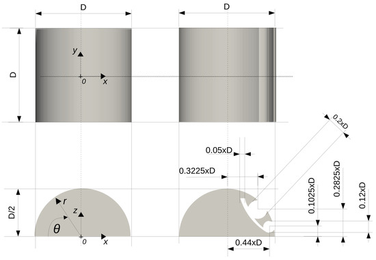
Figure 1.
Key design characteristics of a thick airfoil, with and without Trapped Vortex Cells. x, y, and z are Cartesian coordinates in the longitudinal, vertical, and spanwise directions.
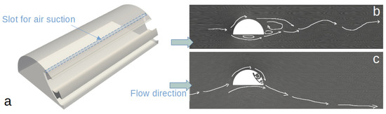
Figure 2.
General view of a bluff body with the integrated aerodynamic flow control system and locations of the surface for air suction (a). The flow mechanics over the thick airfoil (b) and airfoil with AFC (c).
The present concept has been redesigned compared to the initial study [13], resulting in nearly undetached flow past the airfoil. It is important to highlight that this system was developed after several dozen optimization iterations. This concept also abstracts the aerodynamic flow control system for air suction by imposing a fixed pressure drop of Pa, assuming a passive method is employed. In the current model, the consumed air is withdrawn inside the BB, which is not a realistic scenario for real-life applications. However, in a broader context, aircraft dynamics require a feedback control loop in which air suction forcing is dynamically adjusted to achieve optimal system performance. In this context, the present flow control method can be regarded as active. Preliminary studies indicate that increasing the forcing up to allows the flow over the obstacle to remain unseparated while preserving similar large-scale vortex structures in the TVCs. However, this is accompanied by penalties in the form of increased drag force. While further detailed studies are necessary to model realistic air suction using an aircraft engine system, the authors believe that this design serves as a satisfactory proof-of-concept and holds significant potential for further development.
The physics and topology of the flow over BB without trapped vortex cells are qualitatively similar to the flow over a semi-circular cylinder at 50,000, as discussed in detail previously [22]. At a Reynolds number of 130,000, the separation of the laminar boundary layers occurs in the sub-critical flow regime. This condition results in complex, nonlinear interactions between near and far wakes characterized by two types of flow instabilities (Figure 2b). The Kelvin–Helmholtz instability of the separated shear layer, along with vortex shedding (Bénard/von Kármán instability), dominates the wake. Figure 2c shows the schematic flow over the BB with integrated vortex cells. Unlike the initial study [13], this design completely rearranges the flow over the airfoil, making it predominantly unseparated.
2.2. Overview of the Large Eddy Simulation Technique
The Favre-filtered balance equations for mass, momentum, and energy are expressed as follows:
The symbols , p, and represent the density, pressure, and velocity, respectively. Enthalpy per unit mass, h, is given by , with as internal energy per unit mass and T as temperature. The notations , , and represent the Reynolds-averaging, Favre-averaging, and filtering operations, respectively.
The conductive flux and viscous stresses are expressed as follows:
and
where the rate-of-strain tensor, , is:
Here, viscosity, , is calculated by Sutherland’s law and the –conductivity.
For completeness, a filtered equation of state (EoS) is provided to close the system of governing equations using the ideal gas law as follows:
Assuming the sub-grid scales incompressibility hypothesis [24,25], the SGS stress and heat flux can be expressed as follows:
For closure, the k-equation eddy viscosity SGS model [26,27,28] and its dynamic version are used, based on the SGS kinetic energy, . The SGS turbulence stresses are expressed as follows:
with SGS viscosity computed as follows:
where is the filter length. The transport equation used to estimate is as follows:
where production , diffusion , and dissipation are expressed as follows:
Here, is the unit tensor, is the density-weighted stress tensor, is the deviatoric part of the rate of the strain tensor, and the model coefficients are and [29]. The dynamic modification, which is used in the present study, can be derived using the Germano identity with another filter kernel of width (the theoretical background can be found in [24]).
2.3. Ultimate Analytical Lift Properties of Airfoils in Potential Flows
Analogous to knowing the limits in thermodynamics to understand what is possible, knowing the limits in aerodynamics helps us to estimate the maximum lift we can achieve [30]. For this purpose we follow the analysis by Smith [30], when the inviscid potential flows where separation will not occur are assumed and the Joukowski airfoil theory is applicable, expressed as follows:
where is the angle of attack and is the angle determining the maximum airfoil curvature, , where f is the max airfoil curvature and D represents the cord of the airfoil. It is worth noting that Equation (19) is valid when the Chaplygin–Joukowski condition is met at the trailing edge of the airfoil. The given dependencies make it possible to estimate several limiting cases of the lift coefficient for different geometrical shapes as follows:
- —flow around a flat-plate airfoil installed at a given angle of attack (see Figure 3a): . The max theoretical value of the lift force of a thin plate is achieved at the angle of attack, ,
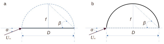 Figure 3. Geometrical parameters of an idealized airfoil: a flat-plate (a) and half-circle (b).
 - —flow around a curved plate in the form of a half-circle (see Figure 3b). In this case, the following values of can be obtained:One can see clearly that the maximum lift coefficient can be achieved for . Of course, the value of depends on the length used as a reference. Here, it is assumed that the conventional chord is applied. For a circle, under the imposed assumptions, it is possible to recover as a limit. In the same spirit, the half-circle limit of can be considered. That is the limiting value for any single-element airfoil [30].
Critical remark. This analysis does not consider the effects of the Mach number. As speed increases, high values of the lift coefficient () cannot be sustained indefinitely, because the surface pressures would soon drop below absolute zero.
3. Brief Aspects of the Numerical Simulations
This section provides a concise overview of the numerical method, along with descriptions of the computational domain, grids, boundary, and initial conditions.
3.1. Overview of the Numerical Methodology
Large eddy simulation is performed using the CFD platform Ansys Fluent 2021R1 [31] (hereinafter, AF). To close the filtered, Favre-averaged Navier–Stokes equations, the dynamic modification of the differential subgrid scale model for the turbulence kinetic energy (k-model) is used. The numerical platform is based on the finite volume method (FVM) implemented as a pressure-based solver [32] using a limited central differencing scheme of the second-order (bounded CDS-2) for the velocity, a second-order upwind scheme (SOU) for the remaining nonlinear convective terms and an implicit Euler method (bounded BDF-2) for time integration [24]. The time integration step is chosen to ensure that the local Courant number is less than one, . The system of linear algebraic equations is solved using the algebraic multigrid method (AMG) accompanied by the additive correction strategy [33] and the classical iterative Gauss–Seidel procedure.
The compressible Reynolds-averaged Navier–Stokes (RANS) equations are solved using the factorized FVM with a second order accuracy in space and time. The linear system of equations is solved in the same manner as in LES. All convective terms are approximated using the SOU scheme. To close the system of the Favre-averaged Navier–Stokes equations, the realizable k- turbulence model of Shih [34] (RKE hereafter) is used. The reader can find more details in [35]. For the inviscid simulation, the system of Euler equations for a perfect gas with the heat capacity ratio, , is solved using the Godunov-type FVM solver [36], where inviscid fluxes are computed using the advection upstream splitting method (AUSM) [37].
A near-wall modeling method was implemented as follows. For the LES, wall functions were used to blend the laminar sublayer and the logarithmic laws proposed by Kader [38]. The RANS approach employed a wall treatment combining a two-layer model with enhanced wall functions. This method maintains the accuracy of the standard two-layer approach for fine near-wall meshes while minimizing accuracy loss for wall-function meshes. The two-layer approach assumes that the computational domain is divided into viscosity-affected and fully turbulent regions. The demarcation is determined by a wall-distance-based turbulent Reynolds number, , with the wall-normal distance, y, calculated at the cell centers. In the fully turbulent region ( > 200), the standard RKE model is utilized. In the viscosity-affected near-wall region, the one-equation model by Wolfshtein [39] is applied, where the computation of turbulent viscosity is modified by introducing a length scale parameter proposed by Chen and Patel [40]. Finally, the blending between the two regions is computed using the method proposed by Jongen [41].
3.2. Computational Grids
Numerical simulations of the turbulent flow over a semi-circular cylinder were conducted using an unstructured, hexahedral-dominated grid with various levels of adaptation (referred to as H0 and displayed in Figure 4). The computational domain was defined as a rectangular parallelepiped with dimensions in the x, y, and z directions, respectively. Initially, the computational block was divided into nodes. Subsequently, the region from to was adapted with a coefficient of . Next, the region from to was refined using a uniform cell size of . The rectangular region with dimensions from to and from to was constructed using a uniform cell size of . Finally, the last rectangular block with dimensions from to and from to was refined using a uniform cell size of . Grid adaptation at all levels covered the computational region in the spanwise direction comprehensively. To adequately resolve the boundary layer of the BB, a viscous sub-grid was added with a minimum dimensionless cell height of , an expansion factor of , and a total of 20 layers. The total grid size amounted to cells.
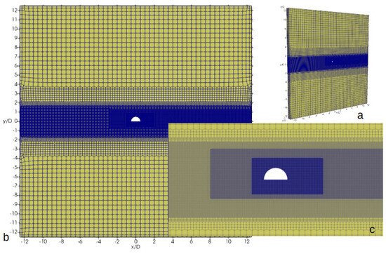
Figure 4.
General view of the baseline mesh and computational domain (a,b) and its frontal view and zoom in the vicinity of a semi-circular cylinder (c).
The unstructured, hexahedral-dominated grid used to simulate the flow over the BB with the implemented aerodynamic flow control was designed similarly to the grid for the semi-circular cylinder (referred to as A0 and presented in Figure 5). The computational domain was defined as a rectangular block with dimensions , initially seeded with nodes in the x, y, and z directions, respectively. The region from to was refined with a coefficient of at the next level. The block from to was further refined using a uniform cell size of . Finally, the cylindrical region with a radius of , located at the center of the Cartesian coordinates, was meshed with a uniform cell size of . A viscous sub-grid was added to the obstacle with averaged , an expansion factor of , and a total of five layers. The total grid size amounted to cells. For the second grid (referred to as A1), the cylindrical region with a radius of was re-meshed with uniform cell sizes of , resulting in a total of cells. Figure 6 displays the probability distribution function (PDF) of and its visualization at the surface of the airfoil for the A1 mesh.
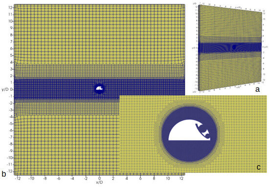
Figure 5.
General view of the baseline mesh and computational domain (a,b) and its frontal view and zoom in the vicinity of the semi-circular cylinder with AFC (c).
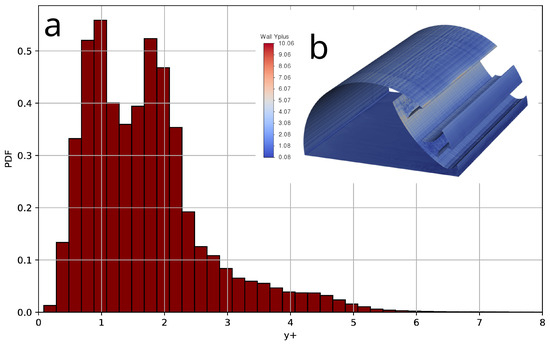
Figure 6.
PDF of (a) and its iso-contours (b) at the surface of the bluff body with AFC, computed for the mesh A1.
3.3. Boundary and Initial Conditions
The boundary conditions were established to ensure that the free-stream parameters were 130,000 and . For LES, a Fourier-based synthetic turbulence generator by Shur et al. [42], proven effective in the previous work [43], was used to realistically reproduce the turbulent inlet flow, with the subgrid kinetic energy intensity set to . Symmetry conditions were applied on the lateral planes, while non-reflecting conditions were set on the other boundaries of the computational domain. For RANS, inlet turbulence was specified using parameters such as intensity () and hydraulic diameter (D). Fixed values for the free stream velocity and total temperature were set at the inlet boundary, while a fixed static pressure was set at the outlet. The body surface was considered adiabatic with no-slip conditions. Simulation of the air suction from the vortex cell system was implemented by setting a fixed static pressure drop of Pa. The initial conditions corresponded to a sudden stop of the body in the fluid flow, meaning the inlet boundary conditions were initially extended to the entire computational domain. The ideal gas law was used to account for compressibility, with constant molecular viscosity and thermal conductivity. The Prandtl number was taken to be , and the ratio of specific heat capacities was .
4. Results
The results section is divided into two main parts. The first part discusses the baseline large-eddy simulations, while the second part examines the viscous effects for the developed concept using the RANS approach.
4.1. LES Results
In this section, the main results for BB with aerodynamic flow control using LES on the A0 and A1 grids are analyzed, and they are indexed as LES-AFC-A0 and LES-AFC-A1, respectively. Furthermore, the complementary run for the semi-circular cylinder without AFC, HC-LES-H0, based on the H0 grid is added for the purpose of comparison.
The characteristic convective time, , is defined as the ratio of the streamwise length of the computational domain () to the free-stream velocity (), represented as . The solution is considered statistically converged when exceeds 3. To ensure statistically independent data, time averaging is conducted over an interval of , with the averaging operator denoted as ⟨⟩.
The main results are presented in Table 1 and Figure 7, Figure 8, Figure 9, Figure 10 and Figure 11. Figure 7 shows the visualization of the instantaneous velocity field using the Q-criterion, clearly depicting the turbulent flow over the object with implemented AFC. Figure 8a,b displays the time-averaged flow field using the LIC (Line Integral Convolution) technique, demonstrating completely non-separated flow over the concept. Figure 9 shows the mean values of the streamwise velocity () and its fluctuations () along the central axial section. For comparison, the values of and obtained for the flow past a circular cylinder for 130,000 ([23]), a semi-circular cylinder for 50,000 ([22]), as well as the available experimental data are gathered. The practically unperturbed flow field over the new concept with AFC predicted numerically is clearly visible. Figure 10 shows the one-dimensional energy spectra of the velocity magnitude obtained at the centers of vortex cells and in the near wake. The spectra obtained on grids A0 and A1 are practically identical, agree well with the universal power law of , and also show the absence of any characteristic low-frequency oscillations associated with vortex dynamics, both in the near wake and in the trapped vortex cells.

Table 1.
Main results: the mean drag, lift coefficients, and aerodynamic quality.
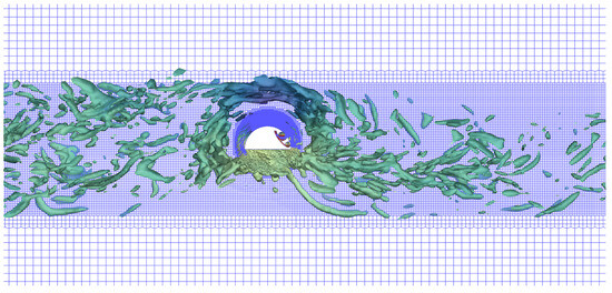
Figure 7.
Instantaneous flow visualization over the BB with an integrated aerodynamic control system (LES-AFC-A1) at 130,000. Iso-surfaces of the Q-criterion (, where S is the strain rate and is the vorticity).
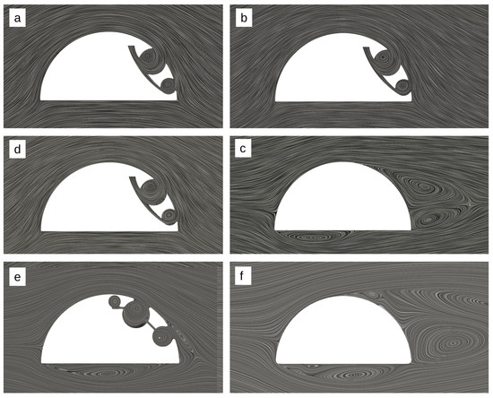
Figure 8.
LIC visualization of the the flow over a bluff body with an integrated aerodynamic control system at 130,000: LES-AFC-A0 (a), LES-AFC-A1 (b), and LES-HC-H0 (c). LIC flow pattern for the specific case using an inviscid gas assumption, when (d). Result visualizations from the original studies: LES-AFC02 [13] (e) and LES-HC2-dTKE [21] (f) at 50,000.
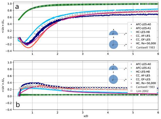
Figure 9.
Distribution of the mean streamwise velocity (a) and its RMS values (b) along the central axis for the flow over a bluff body with and without AFC at 130,000. Supplementary data are provided for HC at 50,000 [22] and CC at 130,000 [23], respectively. Experimental data are included from Cantwell and Coles [44] and Lim and Lee [45].
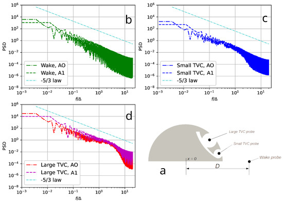
Figure 10.
One-dimensional energy spectra of the velocity magnitude computed for an obstacle with AFC at 130,000: general scheme (a) of the measurement probe locations in the near wake (b) and in the centers of the trapped vortex cells (c,d).
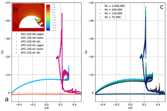
Figure 11.
Distribution of the mean pressure coefficient (a) over the lower (pressure), top (suction), and AFC surfaces of the design with AFC at 130,000, obtained by AFC-LES-A0 and AFC-LES-A1; iso-contours of the mean pressure coefficient (b); and dependence of the mean pressure coefficient from the Reynolds number (c), computed using the RANS approach.
The mean aerodynamic coefficients obtained in both simulations for the concept with AFC were and . It is significant that both parameters obtained using two computational grids, A0 and A1, practically coincide, indicating satisfactory grid independence of the results. LES for the semi-circular cylinder reveals and . Figure 11a shows the distribution of the time-averaged pressure coefficient along the streamwise dimension for the lower (pressure), upper (suction), and AFC system surfaces. The contours of the mean pressure coefficient (Figure 11b) indicate a strong rarefaction formed above the upper surface of the BB and in the vortex cells, which physically justifies a significant increase in lift. The computed coefficient reaches approximately of the maximum analytical value. It is worth emphasizing that, in practice, the magnitude of the lift also depends on the Mach number (compressibility of the air), which is ignored in this work. All simulations are performed with a Mach number of 0.05, and the analytical predictions for are also made without considering compressibility.
It should be noted that although a significant increase in lift is achieved compared to the BB without AFC, the drag force of the concept is approximately twice that of the semi-circular cylinder. The coefficient is closely related to the energy losses in the AFC system, which in turn depends on the pressure drop required to effectively suction air out of the vortex cells. In this work, the pressure drop was artificially increased by approximately to ensure the stability of numerical simulations. In practice, a smaller or larger pressure drop will result in correspondingly smaller or larger AFC energy losses. The influence of the pressure drop on the stability of the AFC system and its energy losses was not investigated in this work, although it is one of the critical topics for further optimization and development of the concept.
For the sake of completeness, it is valuable to demonstrate the evolution of technology development presented in both the previous studies [13,22] and this research. The primary indicators are summarized in Table 1 and Figure 8. For the semi-circular cylinder without AFC technology, increasing the Reynolds number from 50,000 to 130,000 results in significant changes to the flow pattern. Specifically, the massive detached separation zone and the separation zone attached to the lower surface of the body are reduced by approximately half. This transition is evident in Figure 8f ( 50,000) and Figure 8c ( 130,000), which corresponds to a notable change in the integral aerodynamic coefficients. However, it should be noted that the aerodynamic quality in both cases remains consistently negative, approximately . The transformation of the bluff body flow pattern with the AFC system, as detailed in both the previous study [13] and the current work, can be observed in Figure 8e ( 50,000) and Figure 8b ( 130,000). In the present study, a notable improvement in aerodynamic quality—approximately fourfold—is achieved, alongside the development of a practically unseparated flow.
4.2. Analysis of the Viscous Effects Based on the RANS Approach
It is important to analyze the effects of viscosity on the aerodynamic characteristics of the AFC concept, specifically their dependence on the Reynolds number. To this end, a series of simulations were conducted for the following discrete Reynolds numbers: 75,000, 130,000, 500,000, and 1,000,000, using the classical RANS approach. Additionally, to analyze asymptotic behavior, the limiting case for an inviscid gas was studied by solving the Euler equations.
The main results, presented in Table 2 and Figure 12, analyze the following: (a) influence of two-dimensional versus three-dimensional effects (2D vs. 3D); (b) mesh convergence for the A0 and A1 grids; (c) turbulence modeling, realizable k- [34] vs. Spalart–Allmaras [46] (SA hereafter). The obtained results correlate satisfactorily and show the same trend for the drag and lift coefficients (and consequently, aerodynamic quality), with values increasing smoothly and linearly with increasing Reynolds numbers, reaching an asymptotic value. The lift coefficient comes to its maximum value, approximately of the analytical limit.
Table 2.
Summary of the RANS cases investigating the sensitivity of the AFC concept to the Reynolds number: TM, turbulence model; mesh, 2D, A0 or A1; and , , and K represent the drag, lift coefficients, and aerodynamic quality, respectively.
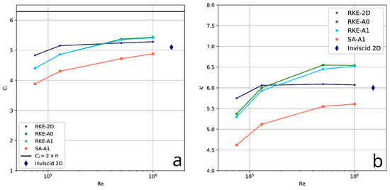
Figure 12.
Reynolds number dependence of the lift coefficient (a) and aerodynamic quality (b)—summary of RANS simulations from Table 2.
To summarize, the following conclusions can be made:
- The results obtained in 2D deviate by approximately 7% from the 3D results for Reynolds numbers of 75,000 and 130,000. As the Reynolds number increases, this discrepancy diminishes.
- There is almost perfect agreement between the baseline simulations using the realizable k- turbulence model on the A0 and A1 grids, indicating grid independence.
- The influence of turbulence models is limited; both RKE and SA models show the same trend but have a systematic shift of around .
- For the limiting case of inviscid fluid, the lift coefficient value is about 5% lower than the values obtained using RKE for a Reynolds number of 1,000,000. This is explained by vortex breakups or the coexistence of small coherent vortex structures in the trapped vortex cells and additional vortices in the system channels, as demonstrated in Figure 8d. The limiting case confirms the general trend.
- From the perspective of numerical modeling, satisfactory agreement is achieved between the aerodynamic coefficients, with a minimum difference of 5% for LES and RANS for a Reynolds number of 130,000. It is important to emphasize that for both approaches, grid dependence of the solution is practically non-existent. The agreement between the results can be attributed to the consistency of both methodologies and the use of a differential, algebraic equation for the kinetic energy to close the Navier–Stokes equations.
5. Discussion
Finally, several important aspects that were not covered in the previous section are discussed here. First, notes on the grid independence study and a complementary comparison of the numerical results obtained using the LES technique and the classical RANS approach are presented. Additionally, a limiting case where , computed using the incompressible setup, is analyzed and compared to its low-Mach-number equivalent ().
5.1. Critical Remark on the Grid Independence Study
In the present work, both LES and RANS simulations were conducted on two grids, A0 and A1. The A1 mesh was specifically designed to refine the central region of the computational domain, which contains the obstacle, by a factor of in all three dimensions. Notably, the primary aerodynamic coefficients computed on these two grids at 130,000 using LES and RANS with the RKE turbulence model demonstrated good convergence, with a relative difference of less than (see Table 1 and Table 2). These results indicate that, at least for 130,000, grid independence was achieved.
The sensitivity analysis of the results with respect to the parameter was extended for the RANS approach. To achieve this, two additional grids were created by refining the first boundary layer attached to the surface of the obstacle, with refinement factors of and . These grids are referred to as A11 and A12, respectively. RANS simulations were conducted using the RKE turbulence model, following a numerical setup consistent with the configurations for grids A0 and A1 at 130,000. Figure 13 presents the probability density functions of for these grids, clearly illustrating a shift in the mean corresponding to the refinement level. Table 3 summarizes the integral aerodynamic coefficients obtained on all grids. The results demonstrate that both the lift and drag coefficients converge well, indicating that the current RANS simulations are largely independent of further refinement beyond the A0 mesh, at least for Re = 130,000.
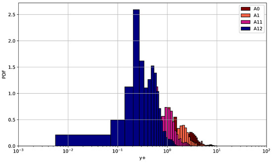
Figure 13.
PDF distributions of at the surface of the bluff body with AFC computed by the RANS approach at 130,000 on different grids.
Table 3.
Effects of the parameter on the integral aerodynamic characteristics of the bluff body with AFC, computed using the RANS approach and the RKE turbulence model at 130,000 on different grids.
5.2. Comparison of Results Obtained by the LES and RANS Approaches
From a systematic perspective, it is insightful to compare the flow patterns computed using two distinct numerical methodologies, namely LES and RANS. For this analysis, two cases are considered as follows: AFC-LES-A1 and AFC-RANS-A1. The integral aerodynamic characteristics, such as and , are presented in Table 1 and Table 2. The results indicate a difference of approximately , with the aerodynamic forces computed by LES being slightly larger. Figure 14 depicts the flow patterns visualized using iso-contours of vorticity magnitude. The primary distinction between LES and RANS lies in the intensity of the vortex cores located within the cells of the AFC system. The vortex cores predicted by LES exhibit significantly higher energy levels, which contribute to slightly larger force coefficients. Figure 15 illustrates the distributions of streamwise velocity obtained from LES and RANS in the wake. The curves align closely, confirming the presence of fully unseparated flow over the obstacle. Overall, the flow patterns computed by LES and RANS are largely identical, except for the differences in vortex core energy. This consistency between the two methods underscores their reliability.
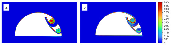
Figure 14.
Iso-contours of the vorticity magnitude at the central cross-section of the computational domain for the flow over a bluff body with AFC, as computed using LES ((a), AFC-LES-A1) and RANS ((b), AFC-RANS-A1) at 130,000.
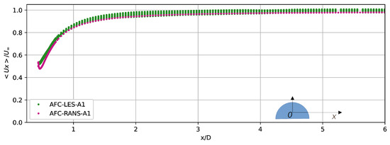
Figure 15.
Distribution of the streamwise velocity along the central axis for the flow over a bluff body with AFC computed by LES and RANS at 130,000.
5.3. Effects of Compressibility
The Mach number is a useful metric for characterizing the significance of compressibility effects [24]. In practice, it is well established that compressibility effects are typically negligible for numerical simulations when . Figure 16 illustrates contours of the Mach number for the RANS case at 130,000 (AFC-RANS-A1). It can be observed that the maximum Mach number reaches at the exit of the AFC system. For the sake of completeness, a special case was conducted for an incompressible fluid (), with the main results presented in Table 2. The data reveal that the differences in drag and lift coefficients between cases for and are approximately . Further investigation of the compressibility effects, specifically the increase in the free-stream Mach number, is beyond the scope of this study and is planned to be investigated in future papers.
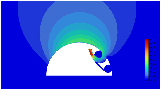
Figure 16.
Iso-contours of the Mach number for the design with AFC at 130,000 obtained by the RANS approach (AFC-RANS-A1).
6. Conclusions
In previous work, the concept of a bluff body with aerodynamic flow control using trapped vortex cells was tested at a Reynolds number of 50,000. This resulted in a significant improvement in lift and aerodynamic quality (from to ) and demonstrated nearly unseparated flow over the body, except for the attached recirculation zone and two saddle-shaped vortices from the lower and lateral surfaces.
In this paper, the concept is further optimized. The free-stream Reynolds number was increased to 130,000, while the Mach number remained the same. To study the properties of the aerodynamic flow control system, the bluff body design was simplified by replacing the lateral surfaces with simple symmetrical planes. Several optimization iterations were conducted to determine the best configuration of the channel and the location of the vortex cells. As a result, nearly non-separating flow over the bluff body was achieved, providing an ultimate lifting force of about of the maximum analytical value (). The lift force of the present design is approximately four times greater than that of the original one [13].
The next logical step was to study the influence of viscosity effects (or Reynolds number). It was shown that the aerodynamic properties of the developed model are practically independent of viscosity effects. Over a wide range of Reynolds numbers (75,000 ≤ Re ≤ 1,000,000), a slight increase in lift and aerodynamic quality (with an almost constant drag coefficient) is observed, with a gradual (linear) approach to an asymptotic value.
It is noteworthy that the aerodynamic drag of the proposed design increased by about compared to a conventional thick airfoil (semi-circular cylinder). This increase is likely due to the consistent pressure drop set in all simulations for air suction from the vortex cells. Additionally, the pressure drop value was slightly increased to ensure the stability of the numerical simulations. The study of the pressure drop’s influence on the aerodynamic characteristics of the object remained beyond the scope of this work but is a fundamental topic for further optimization.
From a numerical modeling perspective, it was interesting to compare the classical RANS approach and the large eddy simulation at a Reynolds number of 130,000. Both methodologies demonstrated a completely unseparated flow around the airfoil with the AFC system. However, a discrepancy of approximately was observed in the aerodynamic coefficients. Further analysis revealed significant differences in the intensities of the vortex cores within the trapped vortex cells. The deviation, spanning several orders of magnitude in vortex core power, accounts for the higher drag and lift coefficient values obtained by LES.
Furthermore, a logical continuation of this work involves studying further the compressibility effects (Mach numbers) and verifying in detail the numerical methodology for critical and super-critical regimes over different bluff bodies.
Funding
This research received no external funding.
Institutional Review Board Statement
Not applicable.
Informed Consent Statement
Not applicable.
Data Availability Statement
Dataset available upon request from the authors.
Conflicts of Interest
Author Dmitry A. Lysenko was employed by the companies 3DMSimtek AS and TechnipFMC. The author declares that the research was conducted in the absence of any commercial or financial relationships that could be construed as a potential conflict of interest.
Abbreviations
The following abbreviations are used in this manuscript:
| AF | Ansys Fluent |
| AFC | Aerodynamic Flow Control |
| AMG | Algebraic Multigrid Method |
| BB | Bluff Body |
| BDF | Backward Differencing Formula |
| CC | Circular Cylinder |
| CDS | Central Differencing Scheme |
| CFD | Computational Fluid Dynamics |
| CRANE | Control of Revolutionary Aircraft with Novel Effectors |
| FVM | Finite Volume Method |
| GAMG | Geometric Multigrid Method |
| HC | Semi-Circular Cylinder |
| LES | Large Eddy Simulation |
| LIC | Line Integral Convolution |
| Probability Density Distribution | |
| RANS | Reynolds-Averaged Navier–Stokes |
| SOU | Second-Order Upwind Scheme |
| TVC | Trapped Vortex Cell |
References
- Joshi, S.N.; Gujarathi, Y.S. A review on active and passive flow control techniques. Int. J. Recent Technol. Mech. Electr. Eng. 2016, 3, 1–6. [Google Scholar]
- Greenblatt, D.; Williams, D.R. Flow control for Unmanned Air Vehicles. Annu. Rev. Fluid Mech. 2022, 54, 383–412. [Google Scholar] [CrossRef]
- Lee, S.; Zhao, Y.; Luo, J.; Zou, J.; Zhang, J.; Zheng, Y.; Zhang, Y. A Review of Flow Control Strategies for Supersonic/Hypersonic Fluid Dynamics. Aerosp. Res. Commun. 2024, 2, 13149. [Google Scholar] [CrossRef]
- Bharghava, D.S.N.; Jana, T.; Kaushik, M. A survey on synthetic jets as active flow control. Aerosp. Syst. 2024, 7, 435–451. [Google Scholar] [CrossRef]
- Mariaprakasam, R.D.R.; Mat, S.; Samin, P.M.; Othman, N.; Wahid, M.; Said, M. Review on flow controls for vehicles aerodynamic drag reduction. J. Adv. Res. Fluid Mech. Therm. Sci. 2023, 101, 11–36. [Google Scholar] [CrossRef]
- Rashidi, S.; Hayatdavoodi, M.; Esfahani, J.A. Vortex shedding suppression and wake control: A review. Ocean Eng. 2016, 126, 57–80. [Google Scholar] [CrossRef]
- Chen, W.-L.; Huang, Y.; Chen, C.; Yu, H.; Gao, D. Review of active control of circular cylinder flow. Ocean Eng. 2022, 258, 111840. [Google Scholar] [CrossRef]
- Derakhshandeh, J.F.; Alam, M.M. A review of bluff body wakes. Ocean Eng. 2019, 182, 475–488. [Google Scholar] [CrossRef]
- Lekkala, M.R.; Latheef, M.; Jung, J.H.; Coraddu, A.; Zhu, H.; Srinil, N.; Lee, B.-H.; Kim, D.K. Recent advances in understanding the flow over bluff bodies with different geometries at moderate Reynolds numbers. Ocean Eng. 2022, 261, 111611. [Google Scholar] [CrossRef]
- Tayebi, A.; Torabi, F. Flow control techniques to improve the aerodynamic performance of Darrieus vertical axis wind turbines: A critical review. J. Wind. Eng. Ind. Aerodyn. 2024, 252, 105820. [Google Scholar] [CrossRef]
- Airforce Technology. X-65 CRANE Demonstrator Aircraft, US. Available online: https://www.airforce-technology.com/projects/x-65-crane-demonstrator-aircraft-us/ (accessed on 20 January 2024).
- Sedda, S.; Sardu, C.; Lasagna, D.; Iuso, G.; Donelli, R.S.; Gregorio, F.D. Trapped vortex cell for aeronautical applications: Flow analysis through PIV and Wavelet transform tools. In Proceedings of the 10th Pacific Symposium on Flow Visualization and Image Processing, Naples, Italy, 15–18 June 2015. [Google Scholar]
- Lysenko, D.A.; Donskov, M.; Ertesvåg, I.S. Large-eddy simulations of the flow past a bluff-body with active flow control based on trapped vortex cells at Re = 50,000. Ocean Eng. 2023, 280, 114496. [Google Scholar] [CrossRef]
- Ringleb, F.O. Separation control by trapped vortices. In Boundary Layer and Flow Control; Lachmann, G.V., Ed.; Pergamon Press: Elmsford, NY, USA, 1961. [Google Scholar]
- Kasper, W. Aircraft Wing with Vortex Generation. U.S. Patent 3,831,885, 27 August 1974. [Google Scholar]
- Kruppa, E.W. A Wind Tunnel Investigation of the Kasper Vortex Concept. In AIAA Paper; American Institute of Aeronautics and Astronautics: Reston, VA, USA, 1977; pp. 77–310. [Google Scholar]
- Savitsky, A.I.; Schukin, L.N.; Karelin, V.G.; Mass, A.M.; Pushkin, R.M.; Shibamov, A.P.; Schukin, I.L.; Fischenko, S.V. Method for Controlling Boundary Layer on an Aerodynamic Surface of a Flying Vehicle. U.S. Patent 5,417,391, 23 May 1995. [Google Scholar]
- Ermishin, A.V.; Isaev, S.A. Flow Control Past Bodies with Vortex Cells Applied to a Blended Wing-Body Aircraft (Numerical and Physical Modeling); St. Petersburg University of Civil Aviation: Saint-Petersburg, Russia, 2024. (In Russian) [Google Scholar]
- Donelli, R.; Gregorio, F.D.; Iannelli, P. Flow separation control by trapped vortex. In Proceedings of the 48th AIAA Aerospace Sciences Meeting Including the New Horizons Forum and Aerospace Exposition, Orlando, FL, USA, 4–7 January 2010; p. 1409. [Google Scholar]
- Isaev, S.A. Aerodynamics of Thickened Bodies with Vortex Cells (Numerical and Physical Modeling); St. Petersburg Polytechnic University: Saint-Petersburg, Russia, 2016. (In Russian) [Google Scholar]
- Lysenko, D.A.; Ertesvåg, I.S. Assessment of algebraic subgrid scale models for the flow over a triangular cylinder at Re = 45,000. Ocean Eng. 2021, 222, 108559. [Google Scholar] [CrossRef]
- Lysenko, D.A.; Donskov, M.; Ertesvåg, I.S. Large-eddy simulations of the flow over a semi-circular cylinder at Re = 50,000. Comput. Fluids 2021, 228, 10505. [Google Scholar] [CrossRef]
- Lysenko, D.A. Large-eddy simulation of the flow past a circular cylinder at Re = 130,000: Effects of numerical platforms and single- and double-precision arithmetic. Fluids 2025, 10, 4. [Google Scholar] [CrossRef]
- Geurts, B. Elements of Direct and Large-Eddy Simulation; R.T.Edwards: Philadelphia, PA, USA, 2004. [Google Scholar]
- Garnier, E.; Adams, N.; Sagaut, P. Large Eddy Simulation for Compressible Flows; Springer: New York, NY, USA, 2009. [Google Scholar]
- Schumann, U. Subgrid scale model for finite difference simulations of turbulent flows in plane channels and annuli. J. Comput. Phys. 1975, 18, 376–404. [Google Scholar] [CrossRef]
- Horiuti, K. Large eddy simulation of turbulent channel flow by one-equation modeling. J. Phys. Soc. Jpn. 1985, 54, 2855–2865. [Google Scholar] [CrossRef]
- Yoshizawa, A. Statistical theory for compressible shear flows, with the application to subgrid modelling. Phys. Fluids 1986, 29, 1416–1429. [Google Scholar] [CrossRef]
- Sagaut, P. Large Eddy Simulation for Incompressible Flows, 3rd ed.; Springer: Berlin, Germany, 2006. [Google Scholar]
- Smith, A.M.P. High lift aerodynamics. In AIAA Paper No. 74939; 1974; Available online: https://charles-oneill.com/aem614/ReferenceMaterial/A+M+O+Smith+HIGH+LIFT+AERODYNAMICS.pdf (accessed on 5 March 2025).
- ANSYS FLUENT 2021SRb. Theory guide. In Tech. Rep.; Ansys Inc.: Canonsburg, PA, USA, 2021.
- Issa, R. Solution of the implicitly discretized fluid flow equations by operator splitting. J. Comput. Phys. 1986, 62, 40–65. [Google Scholar] [CrossRef]
- Hutchinson, B.; Raithby, G. A multigrid method based on the additive correction strategy. J. Numer. Heat Transfer. 1986, 9, 511–537. [Google Scholar]
- Shih, T.H.; Liou, W.; Shabbir, A.; Yang, Z.; Zhu, J. A new k eddy-viscosity model for high Reynolds number turbulent flows—Model development and validation. J. Comput. Fluids 1995, 24, 227–238. [Google Scholar] [CrossRef]
- Lysenko, D.A.; Ertesvåg, I.S.; Rian, K.E. Modeling of turbulent separated flows using OpenFOAM. Comput. Fluids 2013, 80, 408–422. [Google Scholar] [CrossRef]
- Godunov, S.K.; Bohachevsky, I. Finite difference method for numerical computation of discontinuous solutions of the equations of fluid dynamics. Mat. Sb. 1959, 47, 271–306. [Google Scholar]
- Liou, M.-S.; Steffen, C. A new flux splitting scheme. J. Comput. Phys. 1993, 107, 23–39. [Google Scholar] [CrossRef]
- Kader, B. Temperature and concentration profiles in fully turbulent boundary layers. Int. J. Heat Mass Transf. 1981, 24, 1541–1544. [Google Scholar] [CrossRef]
- Wolfshtein, M. The velocity and temperature distribution of one-dimension flow with turbulence augmentation and pressure gradient. Int. J. Heat Mass Transf. 1969, 12, 301–318. [Google Scholar] [CrossRef]
- Chen, H.C.; Patel, V.C. Near-wall turbulence models for complex flows including separation. AIAA J. 1988, 26, 641–648. [Google Scholar] [CrossRef]
- Jongen, T. Simulation and Modeling of Turbulent Incompressible Flows. Ph.D. Thesis, EPF Lausanne, Lausanne, Switzerland, 1992. [Google Scholar]
- Shur, M.L.; Spalart, P.R.; Strelets, M.K.; Travin, A.K. Synthetic turbulence generators for RANS-LES interfaces in zonal simulations of aerodynamic and aeroacoustic problems. Flow Turbul. Combust. 2014, 93, 63–92. [Google Scholar] [CrossRef]
- Lysenko, D.A. Free stream turbulence intensity effects on the flow over a circular cylinder at Re = 3900: Bifurcation, attractors and Lyapunov metric. Ocean Eng. 2023, 287, 115787. [Google Scholar] [CrossRef]
- Cantwell, B.; Coles, D. An experimental study of entrainment and transport in the turbulent near wake of a circular cylinder. J. Fluid Mech. 1983, 136, 321–374. [Google Scholar] [CrossRef]
- Lim, H.-C.; Lee, S.-J. Flow control of circular cylinders with longitudinal grooved surfaces. AIAA J. 2002, 40, 2027–2036. [Google Scholar] [CrossRef]
- Spalart, P.; Allmaras, S. A one-equation turbulence model for aerodynamic flows. In Technical Report AIAA-92-0439; 1992. Available online: https://turbmodels.larc.nasa.gov/Papers/RechAerosp_1994_SpalartAllmaras.pdf (accessed on 5 May 2025).
Disclaimer/Publisher’s Note: The statements, opinions and data contained in all publications are solely those of the individual author(s) and contributor(s) and not of MDPI and/or the editor(s). MDPI and/or the editor(s) disclaim responsibility for any injury to people or property resulting from any ideas, methods, instructions or products referred to in the content. |
© 2025 by the author. Licensee MDPI, Basel, Switzerland. This article is an open access article distributed under the terms and conditions of the Creative Commons Attribution (CC BY) license (https://creativecommons.org/licenses/by/4.0/).