Combination of Integral Transforms and Linear Optimization for Source Reconstruction in Heat and Mass Diffusion Problems

Abstract

This paper presents a novel methodology for estimating space- and time-dependent source terms in heat and mass diffusion problems. The approach combines classical integral transform techniques (CITTs) with the least squares optimization method, enabling an efficient reconstruction of source terms. The method employs a double expansion framework, using both spatial eigenfunction and temporal expansions. The new presented idea assumes that the source term can be expressed as a spatial expansion in eigenfunctions of the eigenvalue problem, and then each transient function associated with each term of spatial expansion is rewritten as an additional expansion, where the unknown coefficients approximating the transformed source enable the direct use of the solution in the objective function. This, in turn, results in a linear optimization problem that can be quickly minimized. Numerical experiments, including one-dimensional and two-dimensional scenarios, demonstrate the accuracy of the proposed method in the presence of noisy data. The results highlight the method’s robustness and computational efficiency, even with minimal temporal expansion terms.

1. Introduction

Playing a fundamental role in various engineering and biomedical applications, Inverse Heat Transfer Problems (IHTPs) aim to estimate unknown parameters or functions, such as thermal properties [1,2,3], boundary conditions [4,5], or heat sources [6,7], based on an observable quantity, most commonly temperature measurements. Several approaches for formulating and solving inverse problems have been extensively developed over the past decades and are compiled in classical compendiums, such as [8,9,10,11,12,13,14]. Inverse problems are known for their ill-posed nature, requiring specific techniques during formulation and solution procedures to ensure regularization and physically meaningful solutions.

The primary motivation for this work is the inverse problem of estimating space- and time-dependent source terms in the diffusion equation. This topic has significant applications across various fields. We can cite application in medicine, where Mehrabanian and Nejad [6] estimate the source term in a bioheat transfer equation to determine the amount of heat needed to eliminate cancerous tissue; in environmental modeling, where Permanoon, Mazaheri, and Amiri [15] propose the inverse problem of reconstructing source terms in a pollutant dispersion model for rivers; also in the context of pollution source identification, Mahar and Datta [16] present excellent results working with groundwater under transient flow and transport conditions; Ling et al. [17] perform inverse estimation of water and fluid leaks from storage tanks and water reservoirs with geomembranes; and Shrivastava and Oza [18] aimed at the identification of origin terms in accidents like Fukushima. Other applications are discussed in [19,20,21,22], among several other works that could be cited.

Many researchers have focused their efforts over the past decades on proposing methodologies that ensure good accuracy in parameter and function estimation, better adaptation to noisy measurements, and diminution of the high computational cost that these inverse problem solutions may require. In the context of source term estimation, we can highlight strategies such as sequential ones [23,24] that include methods like the Kalman filter [25], continuously updating parameter estimates as new measurements are received, ideal for handling dynamic systems and real-time updates, such as capturing moving sources [26]; explicit methods such as presented by Negreiros et al. [27], who developed a methodology based on integral transformation to estimate space- and time-dependent source terms using transformed measurements. Still in the context of using integral transforms for source estimation, Oliveira et al. [7,28] extended this approach and presented studies on three-dimensional problems, incorporating automatic selection of the truncation for the inverse problem solution and extending it to nonlinear diffusive-advective problems. We may also cite the modified polynomial expansion method proposed by Kuo, Liu, and Chang [29], which aims to identify the heat source by discretizing the time and space fields using a characteristic length approach. This method helps stabilize the resulting linear system and ensures a good solution to the inverse problem.

The least squares technique has also played a fundamental role in the context of inverse problems for source term estimation, due to its effectiveness in adjusting parameters to minimize the difference between observed and predicted data in the model [8,12]. Several optimization methods have been integrated into the least squares approach to obtain robust source term estimates, such as the work by Golsorkhi and Tehrani [30], which performs inverse estimation of the source term strength in a one-dimensional conduction problem using an application of the Levenberg–Marquardt method [31,32] with a good convergence rate; Wen, Liu, and Wang [33] combine the conjugate gradient method with a least squares formulation to solve the inverse problem of simultaneously identifying the source term and initial data in time-fractional diffusion problems; and other combinations [34,35].

The inverse problem of source term estimation is typically addressed by analyzing temperature measurements of the phenomenon or system under investigation. These data often contain measurement errors, contributing to the ill-posed nature of the inverse problem—small variations in the input data (measurement noise) are typically amplified in the solution, potentially leading to significant errors in the estimated parameters. Mathematical processes known as regularization methods help stabilize the solution and mitigate these effects. Among the various techniques available in the literature, one can find the Tikhonov regularization [36] is the most classical, which consists of minimizing a functional to determine the smooth solution to the inverse problem. Besides this, we have the Morozov’s discrepancy principle, ref. [37], which defines that the iterative method should be stopped if the discrepancy between the approximate solution and the observed data is approximately equal to the noise level present in the data, as well as Least Absolute Shrinkage and Selection Operator (LASSO) [38] and the singular value decomposition (SVD) method [39]. In the context of regularization of inverse problems, the formulations adopted within the Bayesian inference framework should also be cited, utilizing Markov Random Fields (MRFs) priors for regularization. These formulations provide a robust approach and contribute to solution stabilization [13,40,41].

This work presents a new methodology for estimating space- and time-dependent source terms by combining the classical integral transformation technique (CITT) [42,43] with the least squares optimization method. The key idea is based on the assumption that the source term can be expressed as a spatial expansion in eigenfunctions of the eigenvalue problem, as performed in [7,27]. Each transient function associated with each term of the spatial expansion is then rewritten as an additional expansion, where the unknown coefficients approximating the transformed source enable the direct use of the solution in the objective function. This, in turn, results in a linear optimization problem that can be rapidly minimized, as described in Knupp [1]. Error control in the data is performed using the discrepancy principle to determine the final truncation of the inverse problem solution [27,44].

This article is organized as follows: first, in Section 2, the general formulation of the direct problem and the classical integral transformation technique for its solution are presented; next, in Section 3, the inverse problem of source term estimation is formulated; in Section 4, application examples for one-dimensional and two-dimensional scenarios are provided; finally, in Section 5 and Section 6, the numerical results and the conclusion of the work are presented, respectively.

2. Classical Integral Transform Technique

Given a domain $\Omega$ in ${\mathbb{R}}^n$ with boundary $\partial \Omega$, and considering a time interval $[0,t_{max}]$, the diffusion process is governed by the classical partial differential equation, in a general manner, following the mathematical formulation:

$$w\left(\mathbf{x}\right){\displaystyle \frac{\partial \varphi (\mathbf{x},t)}{\partial t}}-\nabla ·\left[k\left(\mathbf{x}\right)\nabla \varphi (\mathbf{x},t)\right]+d\left(\mathbf{x}\right)\varphi (\mathbf{x},t)=g\left(\mathbf{x},t\right),(\mathbf{x},t)\in \Omega \times (0,t_{max}]$$

(1)

$$\alpha \left(\mathbf{x}\right)\varphi (\mathbf{x},t)+\beta \left(\mathbf{x}\right)k\left(\mathbf{x}\right){\displaystyle \frac{\partial \varphi (\mathbf{x},t)}{\partial \mathbf{n}}}=\xi \left(\mathbf{x},t\right),(\mathbf{x},t)\in \partial \Omega \times (0,t_{max}]$$

(2)

$$\varphi (\mathbf{x},0)=f\left(\mathbf{x}\right),\mathbf{x}\in \Omega ,t=0$$

(3)

where $\varphi (\mathbf{x},t)$ represents the concentration or temperature at position $\mathbf{x}$ and time t, w is the capacity coefficient, k is the diffusion coefficient, d is the linear dissipation coefficient, $\alpha$ and $\beta$ are general boundary condition coefficients, which can be employed to defined first, second, or third kind boundary conditions, $\xi$ is the boundary source term, and $g(\mathbf{x},t)$ is the equation source term that varies arbitrarily in space and time. Even though this differential equation can be directly addressed using the Classical Integral Transform Technique, the convergence of the resulting eigenfunction expansion—measured by the number of terms required to accurately approximate the solution—can be significantly improved by minimizing the influence of the boundary source term, as discussed in ref. [43]. In particular, transforming the problem into a homogeneous boundary condition formulation leads to faster convergence of the series solution, as the non-homogeneous boundary conditions typically introduce slower-decaying modal contributions. Thus, consider the linear filter:

$$\varphi (\mathbf{x},t)={\varphi }_f(\mathbf{x},t)+{\varphi }^{*}(\mathbf{x},t)$$

(4)

in which ${\varphi }_f$ is the simplest possible filter function aimed at homogenizing the boundary condition of the filtered problem formulation, or at least reducing the importance of the boundary source term, where ${\varphi }^{*}$ is the filtered potential. Thus, applying it to Equations (1)–(3), one obtains:

$$w\left(\mathbf{x}\right){\displaystyle \frac{\partial {\varphi }^{*}(\mathbf{x},t)}{\partial t}}-\nabla ·\left[k\left(\mathbf{x}\right)\nabla {\varphi }^{*}(\mathbf{x},t)\right]+d\left(\mathbf{x}\right){\varphi }^{*}(\mathbf{x},t)=g^{*}\left(\mathbf{x},t\right),(\mathbf{x},t)\in \Omega \times (0,t_{max}]$$

(5)

$$\alpha \left(\mathbf{x}\right){\varphi }^{*}(\mathbf{x},t)+\beta \left(\mathbf{x}\right)k\left(\mathbf{x}\right){\displaystyle \frac{\partial {\varphi }^{*}(\mathbf{x},t)}{\partial \mathbf{n}}}={\xi }^{*}\left(\mathbf{x},t\right),(\mathbf{x},t)\in \partial \Omega \times (0,t_{max}]$$

(6)

$${\varphi }^{*}(\mathbf{x},0)=f^{*}\left(\mathbf{x}\right),\mathbf{x}\in \Omega ,t=0$$

(7)

such that

$$g^{*}\left(\mathbf{x},t\right)=g\left(\mathbf{x},t\right)+\nabla ·\left[k\left(\mathbf{x}\right)\nabla {\varphi }_f(\mathbf{x},t)\right]-d\left(\mathbf{x}\right){\varphi }_f(\mathbf{x},t)-w\left(\mathbf{x}\right){\displaystyle \frac{\partial {\varphi }_f(\mathbf{x},t)}{\partial t}}$$

(8)

$${\xi }^{*}\left(\mathbf{x},t\right)=\xi \left(\mathbf{x},t\right)-\alpha \left(\mathbf{x}\right){\varphi }_f(\mathbf{x},t)-\beta \left(\mathbf{x}\right)k\left(\mathbf{x}\right){\displaystyle \frac{\partial {\varphi }_f(\mathbf{x},t)}{\partial \mathbf{n}}}$$

(9)

$$f^{*}\left(\mathbf{x}\right)=f\left(\mathbf{x}\right)-{\varphi }_f(\mathbf{x},t)$$

(10)

The formal solution of the filtered partial differential equation defined by Equations (5)–(7) starts with the definition of a transform–inverse pair, which can be defined as:

$$\mathrm{Transform}:{\overline{\varphi }}_i^{*}\left(t\right)={\int }_{\Omega }w\left(\mathbf{x}\right){\tilde{\psi }}_i\left(\mathbf{x}\right){\varphi }^{*}(\mathbf{x},t)d\Omega$$

(11)

$$\mathrm{Inverse}:{\varphi }^{*}(\mathbf{x},t)=\sum _{i=1}^{\infty }{\overline{\varphi }}_i^{*}\left(t\right){\tilde{\psi }}_i\left(\mathbf{x}\right)$$

(12)

The term ${\tilde{\psi }}_i\left(\mathbf{x}\right)$ present in Equations (11) and (12) represents normalized eigenfunctions obtained through the Sturm–Liouville problem via a direct application of the method of separation of variables to the homogeneous version of Equations (1) and (2):

$$\nabla ·\left[k\left(\mathbf{x}\right)\nabla {\psi }_i\left(\mathbf{x}\right)\right]+\left[{\mu }_i^{2}w\left(\mathbf{x}\right)-d\left(\mathbf{x}\right)\right]{\psi }_i\left(\mathbf{x}\right)=0,\mathbf{x}\in \Omega$$

(13)

$$\alpha \left(\mathbf{x}\right){\psi }_i\left(\mathbf{x}\right)+\beta \left(\mathbf{x}\right)k\left(\mathbf{x}\right){\displaystyle \frac{\partial {\psi }_i\left(\mathbf{x}\right)}{\partial \mathbf{n}}}=0,\mathbf{x}\in \partial \Omega$$

(14)

with norm and the normalized eigenfunctions given, respectively, by:

$$N_i={\int }_{\Omega }w\left(\mathbf{x}\right){\left[{\psi }_i\left(\mathbf{x}\right)\right]}^{2}d\Omega$$

(15)

$${\tilde{\psi }}_i\left(\mathbf{x}\right)={\displaystyle \frac{{\psi }_i\left(\mathbf{x}\right)}{\sqrt{N_i}}}$$

(16)

Operating on Equations (5)–(7) with ${\int }_{\Omega }{\tilde{\psi }}_i\left(\mathbf{x}\right)(·)d\Omega$ yields a system of ordinary differential equations, given by:

$${\displaystyle \frac{d{\overline{\varphi }}_i^{*}\left(t\right)}{dt}}+{\mu }_i^2{\overline{\varphi }}_i^{*}\left(t\right)={\overline{g}}_i^{*}\left(t\right)+{\int }_{A=\partial \Omega }{\displaystyle \frac{{\xi }^{*}\left(\mathbf{x},t\right)\left[k\left(\mathbf{x}\right)\frac{\partial {\tilde{\psi }}_i\left(\mathbf{x}\right)}{\partial \mathbf{n}}-{\tilde{\psi }}_i\left(\mathbf{x}\right)\right]}{\alpha \left(\mathbf{x}\right)+\beta \left(\mathbf{x}\right)}}dA$$

(17)

$${\overline{f}}_i^{*}={\int }_{\Omega }w\left(\mathbf{x}\right){\tilde{\psi }}_i\left(\mathbf{x}\right)f^{*}\left(\mathbf{x}\right)d\Omega$$

(18)

where the transformed source term, represented as ${\overline{g}}_i^{*}\left(t\right)$, is given by:

$${\overline{g}}_i^{*}\left(t\right)={\overline{g}}_i\left(t\right)-{\overline{g}}_i^f\left(t\right)$$

(19)

$${\overline{g}}_i\left(t\right)={\int }_{\Omega }{\tilde{\psi }}_i\left(\mathbf{x}\right)g\left(\mathbf{x},t\right)d\Omega$$

(20)

$${\overline{g}}_i^f\left(t\right)={\int }_{\Omega }{\tilde{\psi }}_i\left(\mathbf{x}\right)\left[-\nabla ·\left[k\left(\mathbf{x}\right)\nabla {\varphi }_f(\mathbf{x},t)\right]+d\left(\mathbf{x}\right){\varphi }_f(\mathbf{x},t)-w\left(\mathbf{x}\right){\displaystyle \frac{\partial {\varphi }_f(\mathbf{x},t)}{\partial t}}\right]d\Omega$$

(21)

Once the solution to the system of Equations (17) and (18) is found, applying the inverse formula Equation (12) yields the solution to the filtered problem defined by Equations (5)–(7):

$${\varphi }^{*}(\mathbf{x},t)=\sum _{i=1}^{\infty }{\tilde{\psi }}_i\left(\mathbf{x}\right)e^{-{\mu }_i^{2}t}\left[{\overline{\varphi }}_i^{*}+{\int }_0^t{e}^{{\mu }_i^2{t}^{\prime }}{\overline{g}}_i^{*}\left(t^{\prime }\right)d{t}^{\prime }\right]$$

(22)

observing the filter Equation (4), the final solution is ultimately obtained by:

$$\varphi (\mathbf{x},t)={\varphi }_f(\mathbf{x},t)+\sum _{i=1}^{\infty }{\tilde{\psi }}_i\left(\mathbf{x}\right)e^{-{\mu }_i^{2}t}\left[{\overline{\varphi }}_i^{*}+{\int }_0^t{e}^{{\mu }_i^2{t}^{\prime }}{\overline{g}}_i^{*}\left(t^{\prime }\right)d{t}^{\prime }\right]$$

(23)

3. Source Term Reconstruction

Consider that the physical problem has an analytical solution given by Equation (23). From a computational perspective, we denote that the calculated temperature $\widehat{\varphi }$ is the solution of Equation (23) truncated with M terms. Thus:

$$\widehat{\varphi }(\mathbf{x},t)={\varphi }_f(\mathbf{x},t)+\sum _{i=1}^M{\tilde{\psi }}_i\left(\mathbf{x}\right)e^{-{\mu }_i^{2}t}\left[{\overline{\varphi }}_i^{*}+{\int }_0^t{e}^{{\mu }_i^2{t}^{\prime }}{\overline{g}}_i^{*}\left(t^{\prime }\right)d{t}^{\prime }\right]$$

(24)

where ${\psi }_i\left(\mathbf{x}\right)$ are eigenfunctions of the eigenvalue problem, defined in Equations (13) and (14).

The objective is to reconstruct the source term $g(\mathbf{x},t)$, treated as unknown in the problem, and here expressed as an eigenfunction expansion on the same basis used to represent the potential, i.e., the one given by the eigenvalue problem in Equations (13) and (14), following the same principle discussed in refs. [7,27,28]. Thus:

$$\widehat{g}(\mathbf{x},t)=\sum _{i=1}^{N_T}{\tilde{\psi }}_i\left(\mathbf{x}\right){\widehat{\overline{g}}}_i\left(t\right)$$

(25)

Differently from refs. [7,27], in the present work, the time-dependent expansion coefficients themselves, ${\widehat{\overline{g}}}_i\left(t\right)$, are represented by a modified classical Fourier expansion with a linear filter, as follows:

$${\widehat{\overline{g}}}_i\left(t\right)={\widehat{\overline{g}}}_{i,0}+{\displaystyle \frac{{\widehat{\overline{g}}}_{i,N_c}-{\widehat{\overline{g}}}_{i,0}}{t_{max}}}t+\sum _{n=1}^{N_c-1}\left({\widehat{\overline{a}}}_{i,n}cos{\displaystyle \frac{n\pi t}{t_{max}}}+{\widehat{\overline{c}}}_{i,n}sin{\displaystyle \frac{n\pi t}{t_{max}}}\right)$$

(26)

with $t\in [0,t_{max}]$. This representation allows for straightforward analytical integration of the integral in Equation (24), yielding an algebraic expression for the calculated potential in terms of constant expansion coefficients of the unknown source term, here denoted as $\mathbf{G}$:

$$\mathbf{G}={[{\widehat{\overline{g}}}_{i,0},{\widehat{\overline{g}}}_{i,N_c},{\widehat{\overline{a}}}_{i,n},{\widehat{\overline{c}}}_{i,n},\dots ]}^T,\mathrm{for}i=1,\dots ,M\mathrm{and}n=1,\dots ,N_c-1.$$

(27)

Assuming experimental measurements of the potential are available, ${\varphi }^e$, at positions $s\in \Omega \times [0,t_{max}]$, the following residuals between calculated values and experimental measurements can be defined for each point s, in terms of the unknown parameters $\mathbf{G}$:

$$R_s\left(\mathbf{G}\right)={\widehat{\varphi }}_s\left(\mathbf{G}\right)-{\varphi }_s^e,s=1,2,\dots N_d$$

(28)

Therefore, for a total of $N_d$ observations, we have:

$$\mathbf{R}=[R_1,R_2,\dots ,R_{N_d}]$$

(29)

thus, the ultimate goal is to minimize the sum of the squared residuals, as defined by the following objective function:

$$\underset{\mathbf{G}\in {\mathbb{R}}^{N_p}}{min}S\left(\mathbf{G}\right)=\sum _{s=1}^{N_d}{R}_s^2$$

(30)

where the vector of unknown parameters $\mathbf{G}$ is determined by minimizing the discrepancy between the model response and the experimental data, as quantified by the objective function $S\left(\mathbf{G}\right)$.

In Equation (30), $N_p$ means the number of parameters to be estimated in $\mathbf{G}$, where it depends on the truncation M and the number of coefficients that make up the temporal expansion $N_c$. That is:

$$N_p=2M{N}_c$$

(31)

The optimal solution to Equation (30) is determined by the Gauss–Newton method [45], initiated through an initial guess ${\mathbf{G}}_0$:

$${\mathbf{G}}_{n+1}={\mathbf{G}}_n-{\left[{\mathbf{J}}_n^T{\mathbf{J}}_n\right]}^{-1}{\mathbf{J}}_n^T\mathbf{R}\left({\mathbf{G}}_n\right),n=0,1,2,3,\dots$$

(32)

in which $\mathbf{J}$ is the sensitivity Jacobian matrix of the coefficients:

$$\mathbf{J}={\displaystyle \frac{\partial \mathbf{R}}{\partial \mathbf{G}}}$$

(33)

with

$$J_{n,j}={\displaystyle \frac{\partial R_n}{\partial G_j}},\mathrm{for}n=1,\dots ,N_d\mathrm{and}j=1,\dots ,N_p.$$

(34)

It is very important to note that, with the representation adopted in this work, the residual vector $\mathbf{R}$ depends linearly on the sought parameters $\mathbf{G}$. Consequently, the sensitivity matrix $\mathbf{J}$ is independent of $\mathbf{G}$, and the iterative procedure in Equation (32) converges with a single iteration [1,46].

To stabilize the inversion in the Gauss–Newton method, we incorporate Tikhonov regularization by adding the term $\lambda \mathbf{I}$ to the system matrix, where $\lambda \in {\mathbb{R}}^{+}$ is a scalar regularization parameter and $\mathbf{I}\in {\mathbb{R}}^{N_p\times N_p}$ is the identity matrix, following the formula below [47]:

$${\mathbf{G}}_{n+1}={\mathbf{G}}_n-{\left[{\mathbf{J}}_n^T{\mathbf{J}}_n+\lambda \mathbf{I}\right]}^{-1}{\mathbf{J}}_n^T\mathbf{R}\left({\mathbf{G}}_n\right),n=0,1,2,3,\dots$$

(35)

This approach helps mitigate issues related to ill-conditioning and improves the robustness of the parameter estimation.

Simulated Data and Error Propagation Control

It is common for real experimental data to be contaminated with measurement errors that naturally occur during the process of obtaining the temperature field. The synthetic data used in the simulations of this work will consider situations where these measurements have errors with a normal distribution of known standard deviation ${\sigma }_e$ and mean $\mu$ equal to zero, as formulated:

$${\varphi }_s^e={\varphi }_s^{\mathrm{num}}+{ϵ}_s,{ϵ}_s\sim \eta (0,{\sigma }_e)$$

(36)

in a manner that ${\varphi }_s^e$ represents the simulated experimental data at position s, ${\varphi }_s^{\mathrm{num}}$ is the numerical solution of the direct problem, and ${ϵ}_s$ is the measurement error, $\eta$, assumed to follow a normal distribution of errors with a mean of 0 and a standard deviation of ${\sigma }_e$. To prevent uncertainties from propagating through the inverse problem solution, the truncation of the solution of Equation (25) is controlled by the discrepancy principle [8,37], where the variance of the data, ${\widehat{\sigma }}^2\left(N_T\right)$, defined by Equation (37), should be close to the known experimental variance ${\widehat{\sigma }}^2\left(N_T\right)\equiv {\sigma }_e^2$.

$${\widehat{\sigma }}^2\left(N_T\right)={\displaystyle \frac{1}{N_d}}\sum _{s\to 1}^{N_d}{\left[{\varphi }_s^e-{\widehat{\varphi }}_s\left(\widehat{g}\right)\right]}^2$$

(37)

Therefore, the selection of the best truncation is performed by minimizing the absolute value of the difference between the estimated variance and the target variance.

In this work, we consider the automatic truncation selection algorithm with the rapid computation of potentials for inverse problems that use the assumption given by Equation (25), as presented in Oliveira et al. [28]. Thus, the automatic selection is determined by the minimum argument of the distance between the computed variance, ${\widehat{\sigma }}^2$, and the target variance, expressed by ${\sigma }_e^2$, which is previously known, as follows:

$$argmin\left|{\widehat{\sigma }}^2\left(N_T\right)-{\sigma }_e^2\right|,N_T=1,2,\dots$$

(38)

where $N_T$ represents the truncation of the solution series for the inverse problem, presented in Equation (25). The estimated potentials for the truncated solution at $N_T$ can be obtained based on the previous truncated solution at $N_T-1$, avoiding redundant calculations by leveraging the orthogonality of the eigenfunction. Thus, the potentials estimated using the recovered source can be obtained by:

$$\widehat{\varphi }(\mathbf{x},t;{\widehat{g}}^{N_T})=\widehat{\varphi }(\mathbf{x},t;{\widehat{g}}^{N_T-1})+\sum _{i=1}^M{\tilde{\psi }}_i\left(\mathbf{x}\right)e^{-{\mu }_i^{2}t}{\int }_0^t{e}^{{\mu }_i^2{t}^{\prime }}\left[{\widehat{\overline{g}}}_{N_T}\left(t^{\prime }\right){\int }_V{\tilde{\psi }}_i\left(\mathbf{x}\right){\tilde{\psi }}_{N_T}\left(\mathbf{x}\right)dV\right]d{t}^{\prime }$$

(39)

where ${\widehat{g}}^{N_T}$ represents the estimated source truncated at $N_T$:

$${\widehat{g}}^{N_T}=\sum _{i=1}^{N_T}{\tilde{\psi }}_i\left(\mathbf{x}\right){\widehat{\overline{g}}}_i\left(t\right)\mathrm{and}{\widehat{g}}^{N_T}-{\widehat{g}}^{N_T-1}={\tilde{\psi }}_{N_T}\left(\mathbf{x}\right){\widehat{\overline{g}}}_{N_T}\left(t\right)$$

(40)

more details can be found in Oliveira et al. [28].

4. Benchmark Examples

4.1. One-Dimensional Case

For the one-dimensional case, considering the geometry ${\Omega }_1=[0,L_x]$ and the classical one-dimensional model for a heat conduction problem, where the potential $\varphi$ here denotes the temperature field, measured in $°\mathrm{C}$ or $\mathrm{K}$:

$${\displaystyle \frac{1}{\alpha }}{\displaystyle \frac{\partial \varphi (x,t)}{\partial t}}-{\displaystyle \frac{{\partial }^2\varphi (x,t)}{\partial x^2}}={\displaystyle \frac{1}{k}}g\left(x,t\right),(x,t)\in {\Omega }_1\times (0,t_{max}]$$

(41)

$${\displaystyle \frac{\partial \varphi (x,t)}{\partial x}}=0,x=0,t\in (0,t_{max}]$$

(42)

$$h\varphi (x,t)+k{\displaystyle \frac{\partial \varphi (x,t)}{\partial x}}=h{\varphi }_{\infty },x=L,t\in (0,t_{max}]$$

(43)

$$\varphi (x,0)={\varphi }_0,t=0$$

(44)

For simplicity, the thermophysical properties are constant and named as follows: the $\varphi [°\mathrm{C}]$ temperature distribution; thermal diffusion coefficient, $\alpha [{\mathrm{m}}^2/\mathrm{s}]$; the thermal conductivity of the material is represented by $k[\mathrm{W}/\mathrm{mK}]$; the heat generation rate (source term) is expressed as $g(x,t)[\mathrm{W}/{\mathrm{m}}^3]$; the convective heat transfer coefficient is indicated by $h[\mathrm{W}/{\mathrm{m}}^2\mathrm{K}]$; ambient temperature is represented as ${\varphi }_{\infty }[°\mathrm{C}]$; and the initial temperature condition is ${\varphi }_0[°\mathrm{C}]$. The length of the material is $L_x\left[\mathrm{m}\right]$, and diffusion occurs over a time interval $[0,t_{max}]\left[\mathrm{s}\right]$. All these terms can be directly associated with the coefficients presented in the general formulation presented in Equations (1)–(3).

The solution of the problem defined by Equations (41)–(44) begins with the simple filter $\varphi (x,t)={\varphi }_{\infty }+{\varphi }^{*}(x,t)$, following the methodology presented in Section 2. Therefore, the solution is obtained:

$$\varphi (x,t)={\varphi }_{\infty }+\sum _{i=1}^M{\tilde{\psi }}_i\left(x\right)e^{-\alpha {\mu }_i^{2}t}\left[{\overline{\varphi }}_i^{*}+{\displaystyle \frac{\alpha }{k}}{\int }_0^t{e}^{\alpha {\mu }_i^2{t}^{\prime }}{\overline{g}}_i\left(t^{\prime }\right)d{t}^{\prime }\right]$$

(45)

in such a way that the transformed source term and the transformed initial condition are represented, respectively, by Equation (46) and Equation (47).

$${\overline{g}}_i\left(t\right)={\int }_{{\Omega }_1}{\tilde{\psi }}_i\left(x\right)g\left(x,t\right)d{\Omega }_1$$

(46)

$${\overline{\varphi }}_i={\int }_{{\Omega }_1}{\tilde{\psi }}_i\left(x\right)\left({\varphi }_0-{\varphi }_{\infty }\right)d{\Omega }_1$$

(47)

The eigenvalue problem associated with the filtered version of the problem has a solution represented by Equation (48), with the transcendental Equation (49) and the inverse of the norm Equation (50).

$${\psi }_i\left(x\right)=cos\left({\mu }_{i}x\right)$$

(48)

$${\mu }_{i}tan\left({\mu }_i{L}_x\right)={\displaystyle \frac{h}{k}}$$

(49)

$${\displaystyle \frac{1}{N_i}}=2{\displaystyle \frac{{\mu }_i^2+{\left(\frac{h}{k}\right)}^2}{L_x\left({\mu }_i^2+{\left(\frac{h}{k}\right)}^2\right)+\frac{h}{k}}}$$

(50)

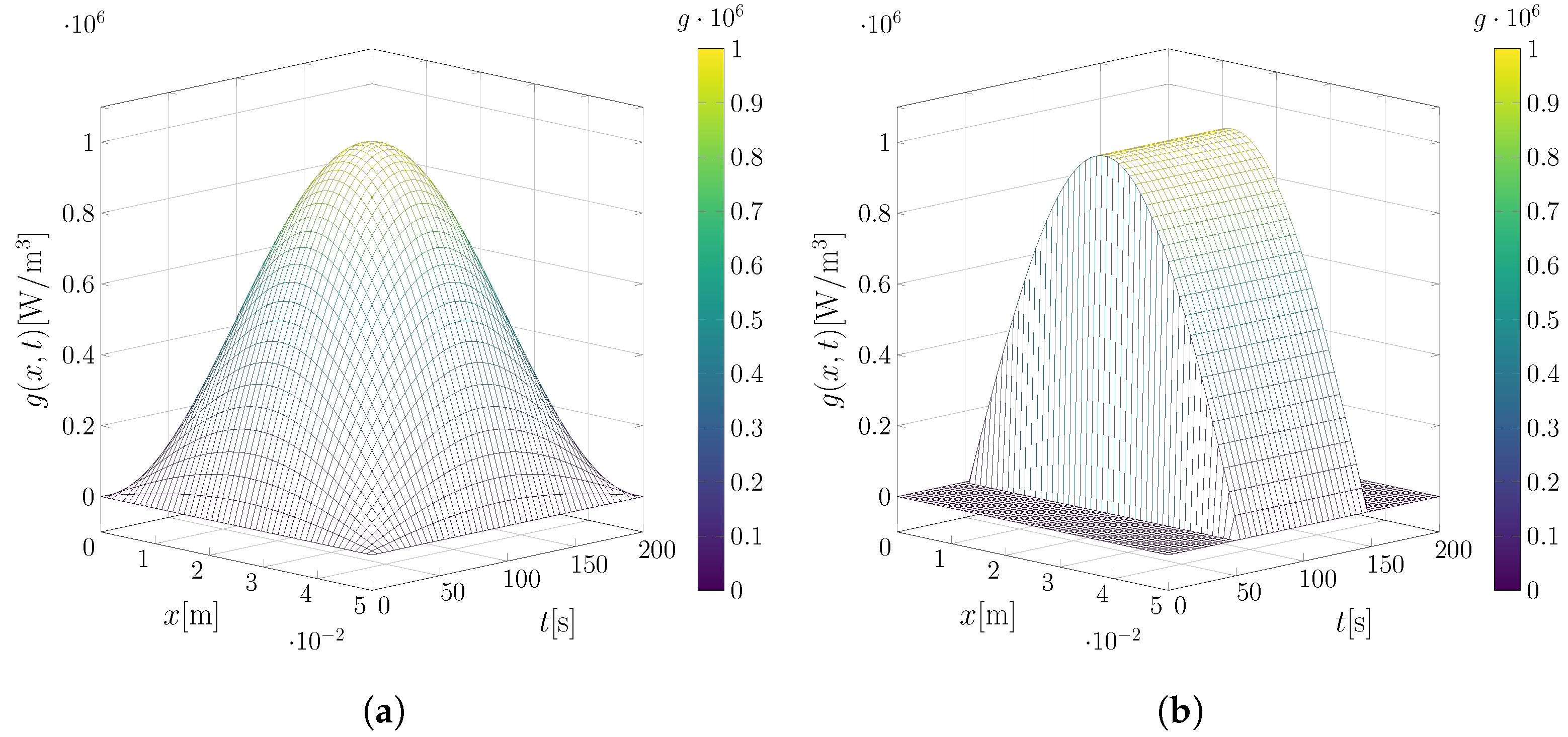
4.2. Two-Dimensional Case

For the two-dimensional case, the inverse problem in transient heat transfer in a plate with heat generation g will be analyzed, subject to boundary conditions that include convection on one edge and thermal insulation on the others. In this case, the domain will be given by ${\Omega }_2=[0,L_x]\times [0,L_y]$, as follows:

$${\displaystyle \frac{1}{\alpha }}{\displaystyle \frac{\partial \varphi (x,y,t)}{\partial t}}-{\nabla }^2\varphi (x,y,t)={\displaystyle \frac{1}{k}}g\left(x,y,t\right),(x,y,t)\in {\Omega }_2\times (0,t_{max}]$$

(51)

$$h\varphi (x,y,t)+k{\displaystyle \frac{\partial \varphi (x,y,t)}{\partial x}}=h{\varphi }_{\infty },\mathrm{at}x=L_x,t\in (0,t_{max}]$$

(52)

$${\displaystyle \frac{\partial \varphi (x,y,t)}{\partial \mathbf{n}}}=0,\mathrm{at}x=0,y=0,\mathrm{and}y=L_y,t\in (0,t_{max}]$$

(53)

$$\varphi (x,y,0)={\varphi }_0,t=0$$

(54)

The solution to this problem starts with the use of the filter for the initial condition formulated as $\varphi (x,y,t)={\varphi }_{\infty }+{\varphi }^{*}(x,y,t)$. Then, the solution to the problem is:

$$\varphi (x,y,t)={\varphi }_{\infty }+\sum _{i=1}^M{\tilde{\psi }}_i(x,y)e^{-\alpha {\mu }_i^{2}t}\left[{\overline{\varphi }}_i^{*}+{\displaystyle \frac{\alpha }{k}}{\int }_0^t{e}^{\alpha {\mu }_i^2{t}^{\prime }}{\overline{g}}_i\left(t^{\prime }\right)d{t}^{\prime }\right]$$

(55)

where

$${\overline{g}}_i\left(t\right)={\int }_{{\Omega }_2}{\tilde{\psi }}_i(x,y)g\left(x,y,t\right)d{\Omega }_2$$

(56)

$${\overline{\varphi }}_i={\int }_{{\Omega }_2}{\tilde{\psi }}_i(x,y)\left({\varphi }_0-{\varphi }_{\infty }\right)d{\Omega }_2$$

(57)

and the solution to the bi-dimensional eigenvalue problem is given by:

$${\psi }_i(x,y)=X_p\left(x\right)Y_q\left(y\right)$$

(58)

where $X_p\left(x\right)$ and $Y_q\left(y\right)$ represent solutions of the problem using the method of separation of variables, with solutions given by [42]:

$$X_p\left(x\right)=cos\left({\zeta }_{p}x\right),Y_q\left(y\right)=cos\left({\gamma }_{q}y\right)$$

(59)

so that ${\zeta }_p$ are the eigenvalues of the eigenvalue problem in the variable x and ${\gamma }_q$ are the eigenvalues of the eigenvalue problem in the variable y, which can be obtained from:

$${\zeta }_{p}tan\left({\zeta }_p{L}_x\right)={\displaystyle \frac{h}{k}},{\gamma }_q={\displaystyle \frac{(q-1)\pi }{L_y}}$$

(60)

The eigenvalues associated with the eigenfunctions ${\psi }_i$, represented by ${\mu }_i$, will be determined by:

$${\mu }_i^2={\zeta }_p^2+{\gamma }_q^2$$

(61)

The eigenvalues are reordered so that the smallest values of ${\mu }_i$ are used first in the final solution, achieving convergence gains [43].

5. Numerical Results

The experimental measurements were simulated using the numerical differential equations solver routine NDSolve from the symbolic computation platform Wolfram Mathematica [48], version 11.3, using the finite element method.

To quantify the accuracy of the estimated source terms, the root mean square error (RMSE) between the estimated and exact sources was calculated using:

$$g_{\mathrm{RMSE}}=\sqrt{{\displaystyle \frac{1}{N_d}}\sum _{s=1}^{N_d}{\left[{\widehat{g}}_s-g_s\right]}^2}$$

(62)

where s represents each simulated experimental measurement location in space and time, and $N_d$ is the total number of observed measurements. The RMSE provides a robust metric to evaluate the fidelity of the estimated compared to the exact source term, enabling a detailed analysis of the method’s performance.

The following presents the numerical results of the estimates for some reference cases of the one-dimensional and two-dimensional models, as described in Section 4.1 and Section 4.2. In all cases, the modified Fourier expansion, represented by Equation (26), was considered, with $N_c=15$.

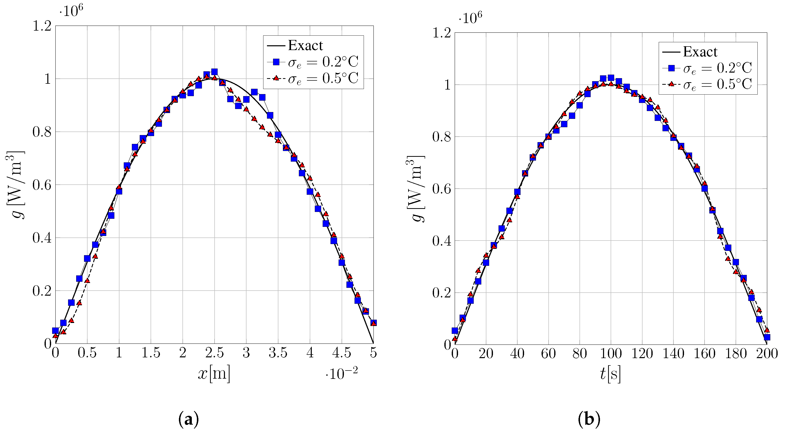
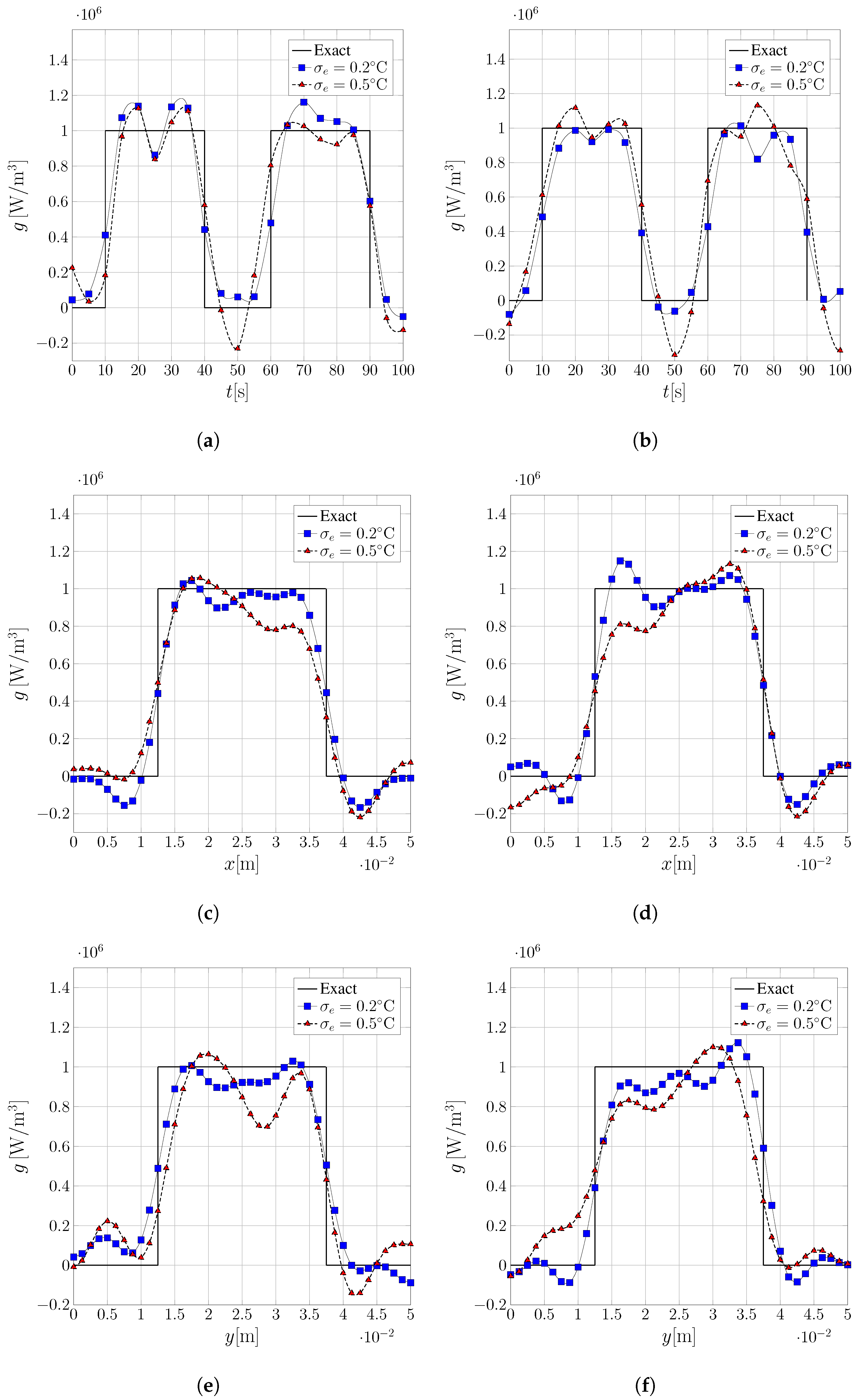
5.1. One-Dimensional Analysis

In the one-dimensional case, we consider the parameters defined in the work by Negreiros et al. [27], given by ${\Omega }_1=[0,0.05\mathrm{m}]$, ${\varphi }_0=30°\mathrm{C}$, ${\varphi }_{\infty }=20°\mathrm{C}$, $h=100\mathrm{W}/{\mathrm{m}}^2\mathrm{K}$, $\alpha =1.153\times {10}^{-7}{\mathrm{m}}^2/\mathrm{s}$, and $k=0.2\mathrm{W}/\mathrm{mK}$ and the sources:

$$\mathit{Source} \mathit{I}:g(x,t)={10}^{6}sin\left({\displaystyle \frac{\pi t}{200}}\right)sin\left({\displaystyle \frac{\pi x}{0.05}}\right)\mathrm{W}/{\mathrm{m}}^3$$

(63)

$$\mathit{Source} \mathit{II}:g(x,t)=\left\{\begin{array}{cc}{10}^{6}sin\left({\displaystyle \frac{x\pi }{0.05}}\right),\hfill & 50\le t\le 150\hfill \\ 0,\hfill & \mathrm{otherwise}\hfill \end{array}\right.\mathrm{W}/{\mathrm{m}}^3$$

(64)

In the first analysis, we have the continuous space-time source term given by Equation (63) and represented in Figure 1a, distributed in smooth oscillatory components in both time and space. The maximum time interval of analysis will be $[0,200] \mathrm{s}$, where the source will exhibit peak values of energy supply to the model Equation (41).

For the second analysis, the heat source is modeled as a piecewise function, formulated by Equation (64) and represented in Figure 1b, activated within a specific time interval $50\le t\le 150 \mathrm{s}$, introducing an abrupt variation in heat generation. The spatial distribution is also sinusoidal with an amplitude of ${10}^6$. This type of modeling is frequently used to represent pulsed energy sources.

For the inverse problem, a total of 26 sensors are located along the x-axis, distributed at equally spaced points, starting at $x=0$ and ending at $x=L$. The transient measurements were obtained starting from $t=0\mathrm{s}$ up to $t_{max}=200\mathrm{s}$, at intervals of $8\mathrm{s}$, totaling 26 observations. Thus, the amount of simulated data for the input of the inverse problem is $N_d=676$. The truncation of the direct problem solution, presented in Section 4.1, was considered to be $M=20$, where, as seen in

Table 1. Convergence of CITT solution for the one-dimensional case I with source Equation (63) at $t=100\mathrm{s}$.

$\mathit{t}=100\mathbf{s}$	$\mathit{M}=5$	$\mathit{M}=10$	$\mathit{M}=15$	$\mathit{M}=20$	$\mathit{M}=25$	NDSolve
$x=0.01$	50.64	51.32	51.22	51.23	51.23	51.23
$x=0.02$	64.62	64.40	64.33	64.33	64.33	64.33
$x=0.03$	64.13	64.40	64.33	64.40	64.33	64.33
$x=0.04$	51.12	51.15	51.03	51.05	51.05	51.05
$x=0.05$	25.59	25.57	25.40	25.38	25.36	25.34

and

Table 2. Convergence of CITT solution for the one-dimensional case I with source Equation (64) at $t=100\mathrm{s}$.

$\mathit{t}=100\mathbf{s}$	$\mathit{M}=5$	$\mathit{M}=10$	$\mathit{M}=15$	$\mathit{M}=20$	$\mathit{M}=25$	NDSolve
$x=0.01$	46.22	46.85	46.75	46.76	46.75	46.75
$x=0.02$	57.38	57.17	57.10	57.11	57.10	57.10
$x=0.03$	56.90	57.17	57.11	57.11	57.10	57.10
$x=0.04$	46.68	46.68	46.56	46.58	46.57	46.57
$x=0.05$	24.92	24.91	24.74	24.72	24.70	24.70

, the values start to show stability at the order of ${10}^{-2}$ at $t=100\mathrm{s}$.

The simulated input data for the inverse problem are generated by the numerical solution of the problem presented in Section 4.1 using the NDSolve solution routine, with added noise deviations of ${\sigma }_{\mathrm{e}}=0.2\mathrm{and}0.5°\mathrm{C}$. Each set of simulated data generated for each noise level was used as input for the inverse problem.

Figure 2 and Figure 3 present comparative profiles between the exact source, Equations (63) and (64), and the inverse problem solutions, respectively, with fixed points at the center of the temporal domain, illustrating the estimation along the x-axis (Figure 2a and Figure 3a), and a fixed point ($x=0.025 \mathrm{m}$) at the center of the spatial domain, illustrating the estimation over time (Figure 2b and Figure 3b). It can be observed that the approach effectively captures the characteristics of the proposed sources, even in the case where there is a temporal discontinuity, Equation (64), as represented in Figure 3b. Figure 4 and Figure 5 show the estimated surface plot for the considered noise levels, where the influence of noise is visible between Figure 4a,b for the source in Equation (63), and Figure 5a,b for the source in Equation (64).

Figure 6 illustrates the steps of the regularization process. Figure 6a presents the automatic selection process based on the discrepancy criterion, where the estimates with noise standard deviation ${\sigma }_e=0.2 °\mathrm{C}$ allow the inclusion of a greater number of terms in the solution series. Figure 6b displays the L-curve, which assists in selecting the parameter $\lambda$, ensuring a balance between smoothness and sensitivity of the problem.

Table 3. RMSE for the estimates of Equations (63) and (64) for the one-dimensional case.

	Source I, Equation (63)	Source II, Equation (64)
${\mathit{\sigma }}_{\mathbf{e}}$	${\mathit{g}}_{\mathbf{RMSE}}\mathbf{\times }{\mathbf{10}}^{\mathbf{5}}$	${\mathit{g}}_{\mathbf{RMSE}}\mathbf{\times }{\mathbf{10}}^{\mathbf{5}}$
0.2	0.2205	0.8859
0.5	0.3361	0.9825

presents the RMSE of the inverse problem solution compared to the exact source. It is observed that the source defined by Equation (64) exhibits greater estimation difficulty due to the abrupt changes in the transient part of the source.

These results demonstrate the robustness of the approach presented in this work for source estimation problems in the one-dimensional case.

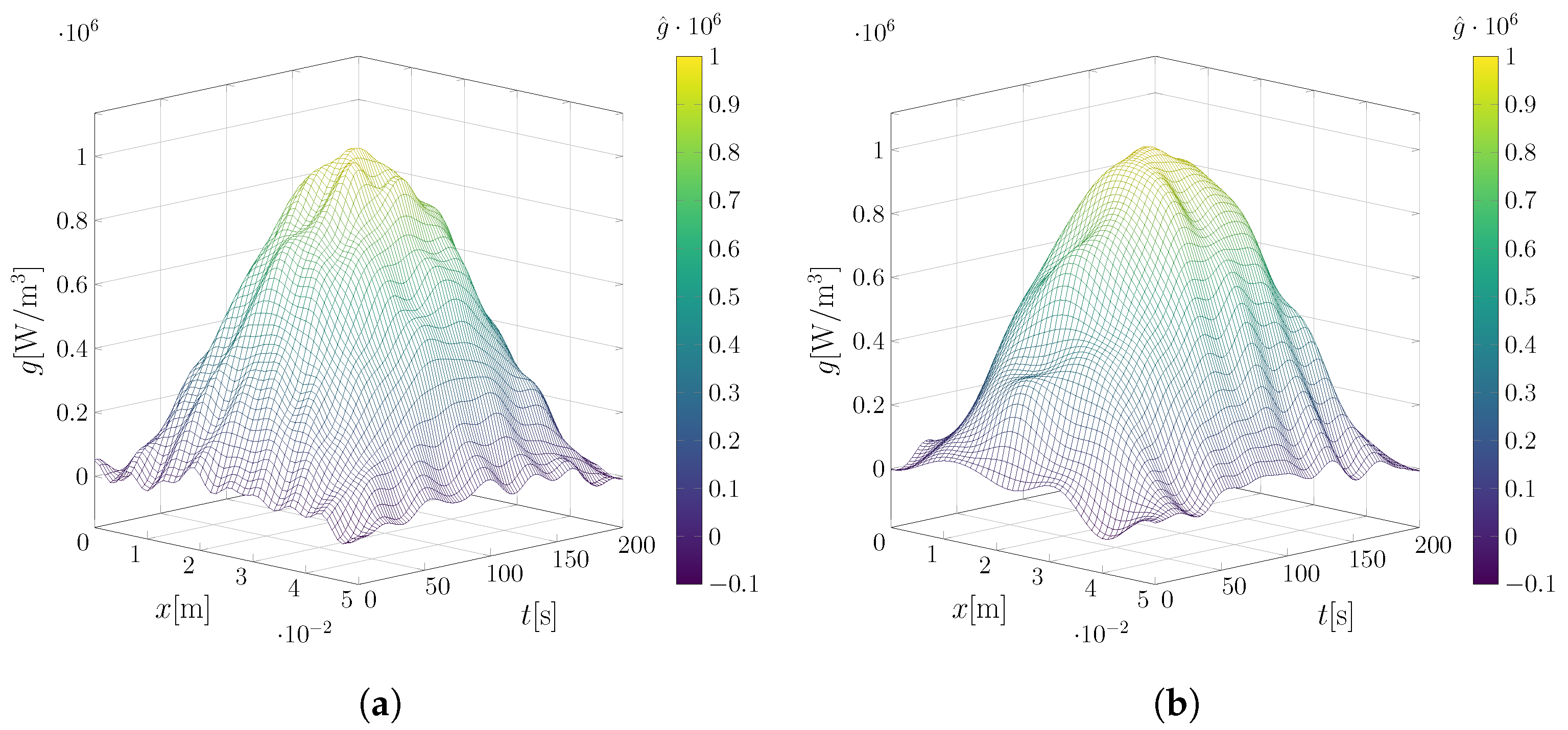
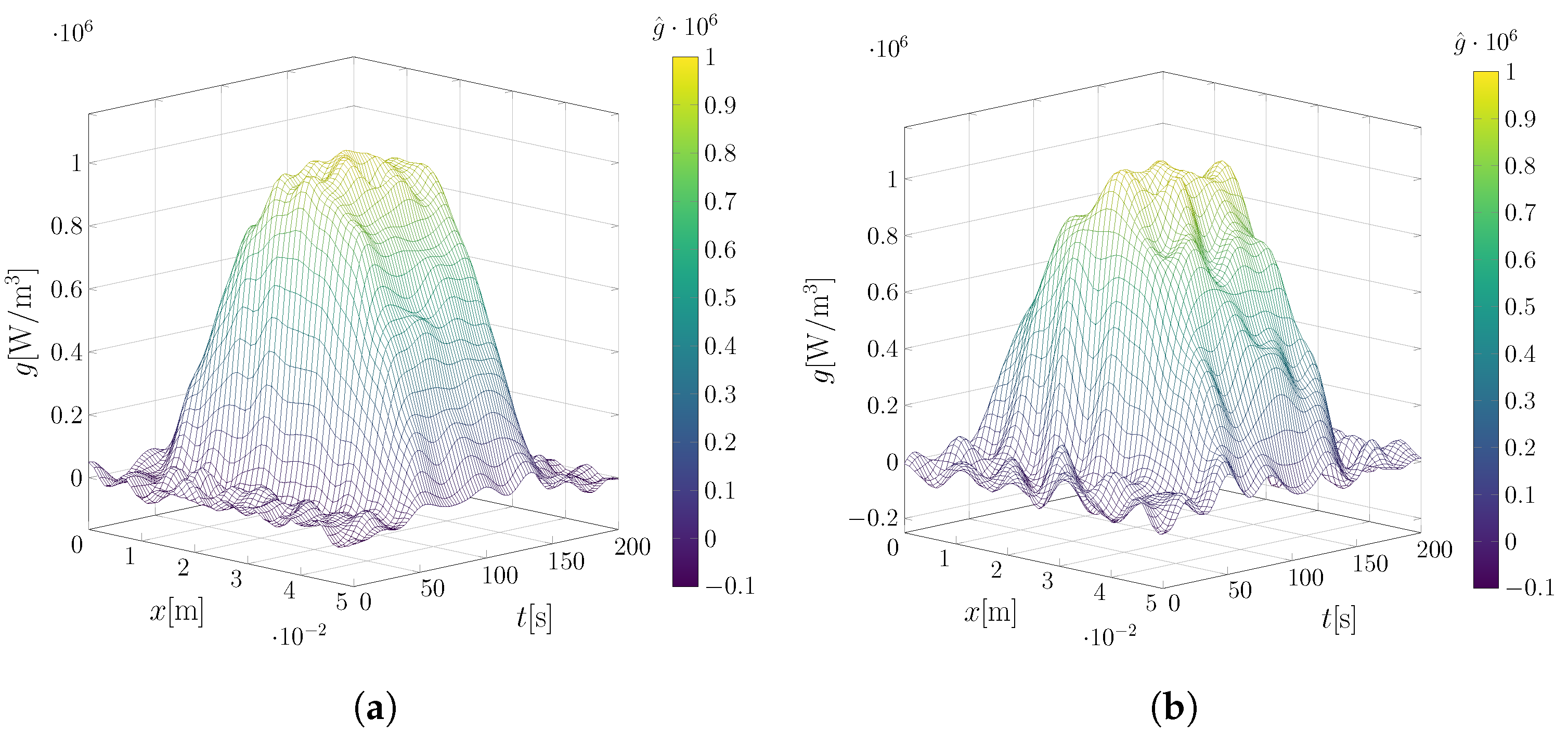
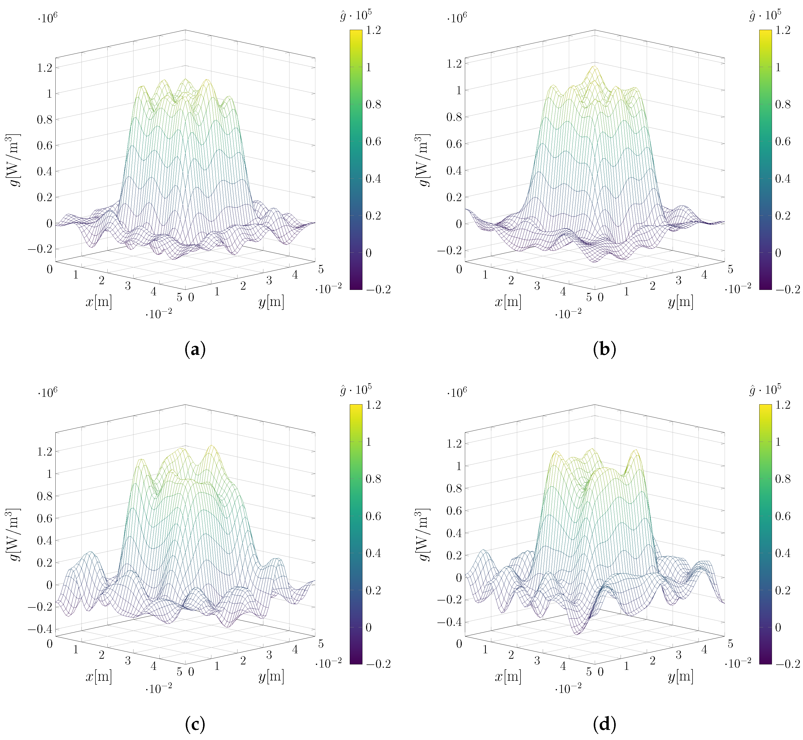
5.2. Two-Dimensional

In the two-dimensional case, we consider the spatial domain ${\Omega }_2=[0,0.05\mathrm{m}]\times [0,0.05\mathrm{m}]$, with ${\varphi }_0=30°\mathrm{C}$, ${\varphi }_{\infty }=20°\mathrm{C}$, $h=15\mathrm{W}/{\mathrm{m}}^2\mathrm{K}$, $\alpha =1.153\times {10}^{-7}{\mathrm{m}}^2/\mathrm{s}$, and $k=0.2\mathrm{W}/\mathrm{mK}$, and the heat source described by Equation (65):

$$g(x,y,t)=\left\{\begin{array}{cc}0,\hfill & 0\le x<0.0125\mathrm{or}x>0.0375\mathrm{and}0\le y<0.0125\mathrm{or}y>0.0375\hfill \\ {10}^{6}q\left(t\right),\hfill & 0.0125\le x\le 0.0375\mathrm{and}0.0125\le y\le 0.0375\hfill \end{array}\right.\mathrm{W}/{\mathrm{m}}^3$$

(65)

where

$$q\left(t\right)=\left(1-2\left|{\displaystyle \frac{t}{100}}-0.5\right|\right)$$

(66)

or

$$q\left(t\right)=\left\{\begin{array}{cc}1,\hfill & \mathrm{if}10\le t\le 40\mathrm{or}60\le t\le 90,\hfill \\ 0,\hfill & \mathrm{otherwise}.\hfill \end{array}\right.$$

(67)

This heat source is characterized by a function that defines a central region in the domain ${\Omega }_2$. Outside this central spatial region, the source term is null, indicating that heat generation is concentrated in a delimited central area, while no generation occurs in the peripheral regions. When the source intensity is defined by Equation (66), the behavior is transient, exhibiting an increasing and decreasing ramp, forming a symmetric triangular profile within the interval $[0,100\mathrm{s}]$. For the source intensity defined by Equation (67), the behavior is pulsed, characterized by abrupt transitions between active and inactive periods over time. This is typical for scenarios where heat generation occurs cyclically or intermittently, such as laser heating processes [49], activation cycles in electronic devices, or biomedical applications with periodic thermal exposure [19,50]. Figure 7 illustrates the spatial behavior when the heat intensities reach their peak values, at $t=50$ s, for Equation (66), for $t=25$ and 75 s, for Equation (67).

In the inverse problem, 11 temperature sensors were considered along each axis x and y, totaling 121 sensors in the plate domain starting at $x,y=0$ and the last ones ending at $x,y=0.05 \mathrm{m}$, and 26 transient observations with intervals of $4\mathrm{s}$, starting at $t=0$ and ending at $t_{max}=100\mathrm{s}$. Now, we considered the solution truncation M was fixed at 120 terms and data contaminated by noise with standard deviations ${\sigma }_{\mathrm{e}}=0.2°\mathrm{C}$ and ${\sigma }_{\mathrm{e}}=0.5°\mathrm{C}$.

Figure 8 presents the estimation results for the heat source, where $q\left(t\right)$ is defined by Equation (66). Figure 8a,b shows the transient estimation profile at two spatial points, while Figure 8c,d illustrates the spatial behavior at $t=50 \mathrm{s}$, the moment when the source reaches its maximum intensity. The corresponding surface plot can be observed in Figure 9.

Similarly to the previously presented results, Figure 10 shows the estimation profiles of the inverse problem for the heat source defined by Equation (67). In Figure 10a,b, it is observed that the transient estimation with a double abrupt transition is well captured by the proposed expansion, preserving its main characteristics. Figure 10c–f presents some spatial estimation profiles at the time instants when the source reaches its maximum value. Figure 11 provides a visualization of the corresponding surface plot.

The graphical results and the RMSE presented in

Table 4. RMSE for the estimates of Equation (65) for the two-dimensional case.

	$\mathit{q}\left(\mathit{t}\right)$ Equation (66)		$\mathit{q}\left(\mathit{t}\right)$ Equation (67)		Tikhonov Parameter
${\mathit{\sigma }}_{\mathbf{e}}$	${\mathit{g}}_{\mathbf{RMSE}}\mathbf{\times }{\mathbf{10}}^{\mathbf{5}}$	${\mathit{N}}_{\mathit{T}}$	${\mathit{g}}_{\mathbf{RMSE}}\mathbf{\times }{\mathbf{10}}^{\mathbf{5}}$	${\mathit{N}}_{\mathit{T}}$	$\mathit{\lambda }$
0.2	0.6248	117	0.6820	118	${10}^{-3}$
0.5	1.3322	93	1.3558	93	${10}^{-3}$

show that the estimation for the noise level ${\sigma }_e=0.2 °\mathrm{C}$ is naturally more accurate, although both estimates are effective in capturing the spatial behavior. Additionally, Table 4 also includes the solution truncation $N_T$, automatically selected, and the Tikhonov regularization parameter.

These results demonstrate the capability of the proposed methodology to reconstruct complex source terms in two-dimensional problems, proving to be efficient and capturing the local and temporal characteristics of the source term effectively.

6. Concluding Remarks

This work introduces a novel methodology for estimating space- and time-dependent source terms using integral transforms combined with the least squares method. The results demonstrate the robustness, accuracy, and computational efficiency of the proposed approach, even in the presence of significant noise in the input data. The test cases, ranging from one-dimensional to two-dimensional scenarios, highlight the method’s ability to handle a wide variety of complex problems.

The main contributions of the proposed method include the ease of implementation due to analytical integrations for the temporal expansion, simplifying its computational implementation. Furthermore, the results indicate high resilience to noise, achieving satisfactory reconstructions even at elevated levels of standard deviation in the data. The modified Fourier expansion for the temporal part of the source term allows the method to adapt to various types of dynamic behaviors, ranging from smooth oscillations to discontinuous or localized effects.

In conclusion, the methodology presented in this work provides a powerful tool for reconstructing source terms in heat transfer problems, with significant potential for adaptation and expansion into new areas of application. The results obtained reinforce the method’s relevance and encourage further exploration of its capabilities.

References

1. Knupp, D.C. Integral transform technique for the direct identification of thermal conductivity and thermal capacity in heterogeneous media. Int. J. Heat Mass Transf. 2021, 171, 121120. [Google Scholar] [CrossRef]
2. Huang, C.H.; Yan, J.Y. An inverse problem in simultaneously measuring temperature-dependent thermal conductivity and heat capacity. Int. J. Heat Mass Transf. 1995, 38, 3433–3441. [Google Scholar] [CrossRef]
3. Yang, C.Y. Determination of the temperature dependent thermophysical properties from temperature responses measured at medium’s boundaries. Int. J. Heat Mass Transf. 2000, 43, 1261–1270. [Google Scholar] [CrossRef]
4. Kubo, S.; Nambu, H. Estimation of Unknown Boundary Values from Inner Displacement and Strain Measurements and Regularization Using Rank Reduction Method. In Inverse Problems in Engineering Mechanics IV; Tanaka, M., Ed.; Elsevier Science B.V.: Amsterdam, The Netherlands, 2003; pp. 75–83. [Google Scholar] [CrossRef]
5. Onishi, K.; Ohura, Y. Direct Method for Solution of Inverse Boundary Value Problem of the Laplace Equation. In Inverse Problems in Engineering Mechanics III; Tanaka, M., Dulikravich, G., Eds.; Elsevier Science Ltd.: Oxford, UK, 2002; pp. 219–226. [Google Scholar] [CrossRef]
6. Mehrabanian, K.; Abbas Nejad, A. A new approach for the heat source estimation in cancerous tissue treatment with hyperthermia. Int. J. Therm. Sci. 2023, 194, 108593. [Google Scholar] [CrossRef]
7. de Oliveira, A.J.; Knupp, D.C.; Abreu, L.A. Integral transforms for explicit source estimation in non-linear advection-diffusion problems. Appl. Math. Comput. 2025, 487, 129092. [Google Scholar] [CrossRef]
8. Alifanov, O. Inverse Heat Transfer Problems; International Series in Heat and Mass Transfer; Springer: Berlin/Heidelberg, Germany, 2012. [Google Scholar]
9. Moura Neto, F.D.; Silva Neto, A.J.d. An Introduction to Inverse Problems with Applications, 1st ed.; Springer: Berlin/Heidelberg, Germany, 2013; pp. XXII, 246. [Google Scholar] [CrossRef]
10. Kirsch, A. An Introduction to the Mathematical Theory of Inverse Problems, 3rd ed.; Applied Mathematical Sciences; Springer: Cham, Switzerland, 2021; pp. XVII, 400. [Google Scholar] [CrossRef]
11. Hasanoğlu, A.H.; Romanov, V.G. Introduction to Inverse Problems for Differential Equations, 2nd ed.; Springer: Cham, Switzerland, 2021; pp. XVII, 515. [Google Scholar] [CrossRef]
12. Beck, J.V.; Arnold, K.J. Parameter Estimation in Engineering and Science; Wiley: New York, NY, USA, 1977. [Google Scholar]
13. Kaipio, J.P.; Somersalo, E. Statistical and Computational Inverse Problems, 1st ed.; Applied Mathematical Sciences; Springer: New York, NY, USA, 2005; Volume 160, pp. XVI, 340. [Google Scholar] [CrossRef]
14. Ozisik, M.N. Inverse Heat Transfer: Fundamentals and Applications; Routledge: London, UK, 2018. [Google Scholar]
15. Permanoon, E.; Mazaheri, M.; Amiri, S. An analytical solution for the advection-dispersion equation inversely in time for pollution source identification. Phys. Chem. Earth Parts A/B/C 2022, 128, 103255. [Google Scholar] [CrossRef]
16. Mahar, P.; Datta, B. Identification of Pollution Sources in Transient Groundwater Systems. Water Resour. Manag. 2000, 14, 209–227. [Google Scholar] [CrossRef]
17. Ling, C.; Revil, A.; Abdulsamad, F.; Qi, Y.; Soueid Ahmed, A.; Shi, P.; Nicaise, S.; Peyras, L. Leakage detection of water reservoirs using a Mise-à-la-Masse approach. J. Hydrol. 2019, 572, 51–65. [Google Scholar] [CrossRef]
18. Shrivastava, R.; Oza, R.B. Development of Kalman Filter Based Source Term Estimation Model (STEM). In Advances in Risk and Reliability Modelling and Assessment; Varde, P.V., Vinod, G., Joshi, N.S., Eds.; Springer: Singapore, 2024; pp. 73–79. [Google Scholar]
19. Baghban, M.; Ayani, M. Source term prediction in a multilayer tissue during hyperthermia. J. Therm. Biol. 2015, 52, 187–191. [Google Scholar] [CrossRef]
20. Bailly du Bois, P.; Laguionie, P.; Boust, D.; Korsakissok, I.; Didier, D.; Fiévet, B. Estimation of marine source-term following Fukushima Dai-ichi accident. J. Environ. Radioact. 2012, 114, 2–9. [Google Scholar] [CrossRef]
21. Luo, J.; Li, X.; Xiong, Y.; Liu, Y. Groundwater pollution source identification using Metropolis-Hasting algorithm combined with Kalman filter algorithm. J. Hydrol. 2023, 626, 130258. [Google Scholar] [CrossRef]
22. Wang, Y.; Chen, B.; Zhu, Z.; Wang, R.; Chen, F.; Zhao, Y.; Zhang, L. A hybrid strategy on combining different optimization algorithms for hazardous gas source term estimation in field cases. Process Saf. Environ. Prot. 2020, 138, 27–38. [Google Scholar] [CrossRef]
23. Massard, H.; Fudym, O.; Orlande, H.; Batsale, J. Nodal predictive error model and Bayesian approach for thermal diffusivity and heat source mapping. Comptes Rendus MéCanique 2010, 338, 434–449. [Google Scholar] [CrossRef]
24. Massard, H.; Orlande, H.R.B.; Fudym, O. Estimation of position-dependent transient heat source with the Kalman filter. Inverse Probl. Sci. Eng. 2012, 20, 1079–1099. [Google Scholar] [CrossRef]
25. Kalman, R.E. A New Approach to Linear Filtering and Prediction Problems. J. Basic Eng. 1960, 82, 35–45. [Google Scholar] [CrossRef]
26. Wang, X.; Zhang, D.; Zhang, L. Estimation of moving heat source for an instantaneous three-dimensional heat transfer system based on step-renewed Kalman filter. Int. J. Heat Mass Transf. 2020, 163, 120435. [Google Scholar] [CrossRef]
27. Negreiros, A.; Knupp, D.; Abreu, L.; Silva Neto, A. Explicit reconstruction of space- and time-dependent heat sources with integral transforms. Numer. Heat Transf. Part Fundam. 2020, 79, 216–233. [Google Scholar] [CrossRef]
28. de Oliveira, A.; Knupp, D.; Abreu, L.; Pelta, D.; Silva Neto, A.J. Improved Inverse Explicit Method for Three-Dimensional Source Term Estimation With the Classical Integral Transform Technique. Asme J. Heat Mass Transf. 2025, 147, 071402. [Google Scholar] [CrossRef]
29. Kuo, C.L.; Liu, C.S.; Chang, J.R. The modified polynomial expansion method for identifying the time dependent heat source in two-dimensional heat conduction problems. Int. J. Heat Mass Transf. 2016, 92, 658–664. [Google Scholar] [CrossRef]
30. Golsorkhi, N.; Tehrani, H. Levenberg-Marquardt Method for Solving the Inverse Heat Transfer Problems. J. Math. Comput. Sci. 2014, 13, 300–310. [Google Scholar] [CrossRef]
31. Levenberg, K. A Method for the Solution of Certain Non-Linear Problems in Least Squares. Q. Appl. Math. 1944, 2, 164–168. [Google Scholar] [CrossRef]
32. Marquardt, D.W. An Algorithm for Least-Squares Estimation of Nonlinear Parameters. J. Soc. Ind. Appl. Math. 1963, 11, 431–441. [Google Scholar] [CrossRef]
33. Wen, J.; Liu, Z.; Wang, S. Conjugate gradient method for simultaneous identification of the source term and initial data in a time-fractional diffusion equation. Appl. Math. Sci. Eng. 2022, 30, 324–338. [Google Scholar] [CrossRef]
34. Su, J.; Hewitt, G. Inverse heat conduction problem of estimating time-varying heat transfer coefficient. Numer. Heat Transf. Part-Appl.-Numer. Heat Transf.-Appl. 2004, 45, 777–789. [Google Scholar] [CrossRef]
35. Tang, C.; Li, S.; Cui, Z. Least-squares-based three-term conjugate gradient methods. J. Inequal. Appl. 2020, 2020, 27. [Google Scholar] [CrossRef]
36. Tikhonov, A.N.; Arsenin, V.I. Solutions of Ill-Posed Problems; Scripta Series in Mathematics, Winston and Distributed Solely; Halsted Press: New York, NY, USA, 1977. [Google Scholar]
37. Morozov, V.A. On the solution of functional equations by the method of regularization. Dokl. Akad. Nauk. Sssr 1966, 167, 510–512. [Google Scholar]
38. Tibshirani, R. Regression shrinkage and selection via the lasso. J. R. Stat. Soc. Ser. B (Methodol.) 1996, 58, 267–288. [Google Scholar] [CrossRef]
39. Hansen, P.C. Rank-Deficient and Discrete Ill-Posed Problems: Numerical Aspects of Linear Inversion; SIAM: Philadelphia, PA, USA, 1998. [Google Scholar]
40. Li, S.Z. Markov Random Field Modeling in Image Analysis, 3rd ed.; Advances in Computer Vision and Pattern Recognition; Springer: London, UK, 2009; pp. XXII, 362. [Google Scholar] [CrossRef]
41. Wang, J.; Zabaras, N. Using Bayesian statistics in the estimation of heat source in radiation. Int. J. Heat Mass Transf. 2005, 48, 15–29. [Google Scholar] [CrossRef]
42. Mikhailov, M.D.; Ozisik, M.N. Unified Analysis and Solutions of Heat and Mass Diffusion; John Wiley and Sons Inc.: New York, NY, USA, 1984. [Google Scholar]
43. Cotta, R.M.; Knupp, D.C.; Naveira Cotta, C.P. Analytical Heat and Fluid Flow in Microchannels and Microsystems; Springer: Berlin/Heidelberg, Germany, 2016. [Google Scholar]
44. Knupp, D.C.; Abreu, L.A. Explicit boundary heat flux reconstruction employing temperature measurements regularized via truncated eigenfunction expansions. Int. Commun. Heat Mass Transf. 2016, 78, 241–252. [Google Scholar] [CrossRef]
45. Hoffmann, J.; Shafer, K. Linear Regression Analysis: Assumptions and Applications; NASW: Washington, DC, USA, 2015. [Google Scholar]
46. Fletcher, R. Practical Methods of Optimization, 2nd ed.; John Wiley & Sons: New York, NY, USA, 1987. [Google Scholar]
47. Hansen, P.C.; Pereyra, V.; Scherer, G. Least Squares Data Fitting with Applications; Johns Hopkins University Press: Philadelphia, PA, USA, 2013. [Google Scholar] [CrossRef]
48. Wolfram Research, Inc. Mathematica, version 13.3; Wolfram Research, Inc.: Champaign, IL, USA, 2023. [Google Scholar]
49. Brown, M.S.; Arnold, C.B. Fundamentals of Laser-Material Interaction and Application to Multiscale Surface Modification. In Laser Precision Microfabrication; Sugioka, K., Meunier, M., Piqué, A., Eds.; Springer Series in Materials Science; Springer: Berlin/Heidelberg, Germany, 2010; Volume 135, pp. 91–120. [Google Scholar] [CrossRef]
50. Remlova, E.; Feig, V.R.; Kang, Z.; Patel, A.; Ballinger, I.; Ginzburg, A.; Kuosmanen, J.; Fabian, N.; Ishida, K.; Jenkins, J.; et al. Activated Metals to Generate Heat for Biomedical Applications. ACS Mater. Lett. 2023, 5, 2508–2517. [Google Scholar] [CrossRef]
Figure 1. Surface of the exact source terms for the one-dimensional cases. (a) Case with  σ e = 0.2 ° C ; (b) case with  σ e = 0.5 ° C .
Fluids 10 00106 g001
Figure 2. Comparison between the exact source term and inverse problem solutions for different noise levels in the input data for the one-dimensional case. (a) Temperature profile at  t = 100 s ; (b) temperature evolution at  x = 0.025 m .
Fluids 10 00106 g002
Figure 3. Comparison between the exact source term Equation (64) and the inverse problem solutions for different noise levels. (a) Temperature profile at  t = 100 s ; (b) temperature evolution at  x = 0.025 m .
Fluids 10 00106 g003
Figure 4. Inverse problem surface solutions for different noise levels in the input data for the one-dimensional case, source term Equation (63). (a) Solution with  σ e = 0.2 ° C ; (b) solution with  σ e = 0.5 ° C .
Fluids 10 00106 g004
Figure 5. Inverse problem surface solutions for different noise levels in the input data for the one-dimensional case, source term Equation (64). (a) Solution with  σ e = 0.2 ° C ; (b) solution with  σ e = 0.5 ° C .
Fluids 10 00106 g005
Figure 6. One-dimensional regularization behaviors for the inverse problem. (a) Regularization based on the discrepancy principle; (b) Tikhonov regularization approach.
Fluids 10 00106 g006
Figure 7. Surface of the two-dimensional exact source term given by Equation (65) with  q ( t )  defined by Equation (66) at  t = 50 s  or  q ( t )  defined by Equation (67) at  t = 25 s  and  t = 75 s .
Fluids 10 00106 g007
Figure 8. Comparison between the exact source term and inverse problem solutions for different noise levels in the input data for the two-dimensional case, with  q ( t )  given by Equation (66). (a) Profile at  x = 0.025 m  and  y = 0.025 m ; (b x = 0.03 m  and  y = 0.03 m ; (c t = 50 s  and  y = 0.015 m ; (d t = 50 s  and  x = 0.015 m .
Fluids 10 00106 g008
Figure 9. Inverse problem surface solutions for different noise levels in the input data for the two-dimensional case, with  q ( t )  given by Equation (66). (a) Case with  σ e = 0.2   ° C ; (b) case with  σ e = 0.5 ° C .
Fluids 10 00106 g009
Figure 10. Comparison between the exact source term and inverse problem solutions for different noise levels in the input data for the two-dimensional case, with  q ( t )  given by Equation (67). (a) Profile at  x = 0.025 m  and  y = 0.025 m ; (b x = 0.03 m  and  y = 0.03 m ; (c t = 25 s  and  y = 0.035 m ; (d t = 75 s  and  y = 0.035 m ; (e t = 25 s  and  x = 0.015 m ; (f t = 75 s  and  x = 0.015 m .
Fluids 10 00106 g010
Figure 11. Inverse problem surface solutions for different noise levels in the input data for the two-dimensional case, with  q ( t )  given by Equation (67). (a t = 25 s  and  σ e = 0.2 ° C ; (b t = 75 s  and  σ e = 0.2 ° C ; (c t = 25 s  and  σ e = 0.5 ° C ; (d t = 75 s  and  σ e = 0.5 ° C .
Fluids 10 00106 g011