Abstract
A transient stability flow analysis is performed using the unsteady laminar boundary layer equations. The flow dynamics are studied via the Navier–Stokes equations. In the case of external spatially developing flow, the differential equations are reduced via Prandtl or boundary-layer assumptions, consisting of continuity and momentum conservation equations. Prescription of streamwise pressure gradients (decelerating and accelerating flows) is carried out by an impulsively started Falkner–Skan (FS) or wedge-flow similarity flow solution in the case of flat plate or a Blasius solution for particular zero-pressure gradient case. The obtained mean streamwise velocity and its derivatives from FS flows are then inserted into the well-known Orr–Sommerfeld equation of small disturbances at different dimensionless times (). Finally, the corresponding eigenvalues are dynamically computed for temporal stability analysis. A finite difference algorithm is effectively applied to solve the Orr–Sommerfeld equations. It is observed that flow acceleration or favorable pressure gradients (FPGs) lead to a significantly shorter transient period before reaching steady-state conditions, as the developed shear layer is notably thinner compared to cases with adverse pressure gradients (APGs). During the transient phase (i.e., for ), the majority of the flow modifications are confined to the innermost 20–25% of the boundary layer, in proximity to the wall. In the context of temporal flow stability, the magnitude of the pressure gradient is pivotal in determining the streamwise extent of the Tollmien–Schlichting (TS) waves. In highly accelerated laminar flows, these waves experience considerable elongation. Conversely, under the influence of a strong adverse pressure gradient, the characteristic streamwise length of the smallest unstable wavelength, which is necessary for destabilization via TS waves, is significantly reduced. Furthermore, flows subjected to acceleration ( > 0) exhibit a higher propensity to transition towards a more stable state during the initial transient phase. For instance, the time response required to reach the steady-state critical Reynolds number was approximately 1 for = 0.18 (FPG) and = 6.8 for = −0.18 (APG).
1. Background
The Navier–Stokes (NS) equations are the basis of fluid mechanics theory. This set of partial differential equations (PDEs) consists of a continuity equation that studies mass transport and momentum equations that study flow dynamics, fluid forces, and acceleration. According to the Clay Mathematics Institute [1], there is not yet an analytical solution to the full Navier–Stokes equations, but there are several solutions to these equation based on assumptions to reduce their complexity. The boundary-layer theory was originally proposed by Prandtl. The solution of the Navier–Stokes equations is achieved by applying the following boundary-layer assumptions: (1) The velocity component parallel to the wall has a much larger magnitude than that of the wall-normal fluid velocity component. (2) The pressure gradient may vary in the direction parallel to the wall; however, the pressure remains constant in the direction perpendicular to the wall. (3) Streamwise gradients can be neglected with respect to wall-normal gradients [2]. Once these assumptions are applied to the NS equations, the Prandtl boundary-layer equations are obtained. In the present scenario, an unsteady problem is assumed, and the effects of time are taken into account. It is important to mention that for incompressible flow, buoyancy is neglected due to the fact that the variation in the flow properties as the pressure and temperature changes is very small and remains quasi-constant, so the energy equation can be decoupled from the momentum equation [3].
As stated earlier, there is a limited number of analytical solutions for the NS equations. In general, these equations are solved numerically (or semi-analytically) by applying finite-difference, finite-volume, and finite-element schemes. The unsteady boundary-layer equations can be solved via similarity analysis by normalizing the streamwise (x), wall-normal (y), and time (t) coordinates using variable and values. According to the fluid mechanics theory, the external flow has three phases: (i) a laminar phase, where the flow exhibits orderly movement with poor resistance to high Reynolds numbers; (ii) a transitional phase, where the flow changes from laminar to turbulent; and (iii) a turbulent flow phase, which is considered an unsteady, chaotic, and disorderly but stable phenomenon at high Reynolds numbers. The Reynolds number is defined as the ratio of the inertial to viscous forces in a fluid flow. In fluid mechanics, it is usually assumed that the flow changes from the laminar to turbulent stage in a typical flat plate at a Reynolds number of 500,000 (i.e., , where is the freestream velocity, x is the streamwise coordinate measured from the leading edge, and is the fluid kinematic viscosity) [2,3]. However, this is just an engineering estimate. In reality, the distance between the streamwise location where a laminar flow becomes unstable, or the instability point (), and the transition endpoint, where the flow becomes fully turbulent, could be very large [3]. It is worth highlighting that, to this day, transitional flow its not very well understood, and there is no theory of transition; therefore, it is generally studied on a case-by-case basis. A flow stability analysis determines the onset of transition, where Tollmien–Schlichting (TS) waves initially form. According to White [3], stability theory studies how a physical system reacts under the influence of small, external disturbances and the onset of instability of fluid flows. Generally speaking, there are four stability types: (i) a system is stable if it returns to its original position after an external disturbance; (ii) unstable if the physical state cannot return to its original position; (iii) neutral or marginally stable if the physical state remains at its original position or goes back to where it started without limit, no matter the disturbance; and (iv) partially stable when the physical state is stable or unstable according to the strength of the external disturbance. This analysis involves the following steps: (1) adding a small disturbance to a selected basic flow solution, (2) isolating the disturbance governing equations, (3) linearizing the equations by assuming small disturbances (thus, higher-order terms can be neglected), (4) modeling disturbances as a traveling wave, and (5) solving the eigenvalues. Applying stability to NS equations results in a traveling wave equation. The assumptions for the transport equations of disturbances are as follows: a two-dimensional incompressible parallel flow, small disturbances, and Squires theorem validity. Moreover, the Squires theorem states that for a 2D parallel flow (), the minimum critical unstable Reynolds number occurs for the case of a two-dimensional disturbance propagated along the same direction, where the wave angle is zero. Therefore, stability analysis performed via the Orr–Sommerfeld equation (OSE) is highly conservative. Finally, once these steps and assumptions are applied to the NS equations, the well-known Orr–Sommerfeld equation (OSE) is obtained.
A substantial amount of work has been done on flow stability. Wazzan et al. [4] presented a set of spatial and temporal stability charts for the steady Falkner–Skan boundary layer incompressible flow raging from a pressure gradient () of to 1. Wazzan et al. [4] solved the Orr–Sommerfeld equation using a step-by-step integration method with a Gram–Schmidt orthogonalization procedure to eliminate the rapid build-up of errors. Their numerical results were in good agreement with the experimental data of Schubauer and Skramstad [5] for the eigenfunction solutions. Ishak et al. [6] investigated the effects of the Falkner–Skan power-law parameter, suction, or injection parameters, as well as the ratio of freestream velocity to the boundary velocity parameter for a moving wedge, concluding that suction delayed separation and separation did not occur when the wedge and fluid moved in the same direction. Simpson [7] developed a Matlab code to solve the temporal and spatial solutions of the Orr–Sommerfeld equation using a finite difference scheme. He stated that for the temporal solution for each wave number () and Reynolds number, the most unstable eigenvalue (in this case, the complex number c, which is the wave propagation speed) must be stored. Simpson [7] also concluded that his results differed slightly from those of [4] because the Orr–Sommerfeld equation was non-dimensionalized with respect to the boundary-layer thickness instead of the displacement thickness. Banks and Drazing [8] solved the Falkner–Skan equation and the problem of hydrodynamic instability by applying a bifurcation solution. Banks and Drazing [8] stated that a small parameter problem is usually solved by expanding the solutions in powers of that parameter. However, in singular cases, the linearized problem is unsolvable, and it is more appropriate to expand the solution in powers of the square root of the small parameter instead. Han [9] developed a finite difference solution of the steady Falkner–Skan equations by separating the third-order differential equation into two ordinary differential equations (one of first order and the other of second order). Han [9] concluded that this method provided a way to solve the steady Falkner–Skan equations without the tedious trial–error steps of the shooting method. Wazzan et al. [10] studied the stability of water boundary-layer flow over a flat plate of a heated and cooled wall by extending the Orr0-Sommerfeld solution to take into account fluid-dependent properties. Wazzan et al. [10] concluded that major factors affecting stability were (i) the shape of the boundary-layer velocity profile or streamwise pressure gradient, (ii) the Reynolds number, and (iii) the wave number or frequency of the disturbance. Govindarajan and Narashima [11] proposed a formulation for flow stability analysis under the effect of streamwise pressure gradients to take into account flow non-parallelism by including a correction of the order of , where R is the Reynolds number. Govindarajan and Narashima [11] stated that an important assumption of the Orr–Sommerfeld equation is that, although the Reynolds number varies with downstream distance (x), the flow may be considered locally parallel (the mean flow variations in x may be ignored). The Orr–Sommerfeld equation is an approximation when compared with experimental measurements where discrepancies can be observed due to non-parallel effects in the flow. It was concluded in [11] that non-parallel flow effects were more prominent in decelerating flows. Bertolotti et al. [12] introduced two techniques for the study of linear and non-linear instability in evolving boundary layers. The first technique employs differential equations of the parabolic type, exploiting the slow change of the mean flow, disturbance velocity profile, wavelength, and growth rates along the streamwise direction. The second technique solves the Navier–Stokes equations for spatially evolving disturbances using buffer zones adjacent to the inflow and outflow boundaries. Bertolotti et al. also stated that the non-parallelism effects are weak and not responsible for the discrepancies between measurement and theoretical results for parallel flow, at least in the analyzed ZPG flow and Blasius solutions. Furthermore, Bertolotti et al. [12] concluded that the effects of flow non-parallelism increased for three-dimensional waves as the direction of the wave propagation veered away from that of the mean flow. In addition, Bertolotti et al. [12] stated that this destabilizing effect in three-dimensional waves was sufficiently strong at higher frequencies to alter the results of Squire’s theorem for parallel flow. Saric et al.’s [13] review paper surveyed three-dimensional boundary-layer stability and transition progress, with a focus on cross-flow instability leading to transition on swept wings and rotating disks. Saric et al. [13] found that in the past decade, several important discoveries have been made, including instrumentation that can be applied to the flight-test environment, POD methods to interpret wind-tunnel and flight-test transition data, and validation of NPSE codes with careful experiments to predict all aspects of stationary disturbance growth. Saric et al. [13] also reported some important factors that affect stability analyses, including environmental conditions on the appearance of stationary and traveling waves, secondary instability causing a local transition in stationary cross-flow-dominated flows, the extreme sensitivity of stationary disturbance to the leading edge, very low surface roughness, and the extreme sensitivity of stationary wave growth to very weak convex curvature. Perez et al. [14] investigated the non-orthogonal incompressible attachment line boundary-layer flow, which is a combination of two-dimensional non-orthogonal and swept boundary-layer flow. Perez et al. [14] used a Biglobal stability analysis and verified it by performing a DNS analysis. Perez et al. [14] also studied the effects of the angle of attack on the critical conditions of the non-orthogonal problem and found that increasing the angle of attack systematically destabilized the flow. Wazzan et al. [15] computed the stability of an incompressible flat-plate boundary layer with a pressure gradient from the linearized small disturbances equations. Wazzan et al. [15] stated that parallel flow is the most common assumption of linear stability analysis, but it is important to mention that only fully developed mean flows bounded by parallel walls are exactly parallel. Spatially developing boundary layers are formed by mean flows where the velocity components in the freestream direction and normal to it vary with the x and y coordinates. Wazzan et al. [15] concluded that non-parallel flow effects have a negligible influence on the critical Reynolds number for pressure gradients () between 0.4 and 1.0 but lead to a slight decrease in the critical Reynolds number for pressure gradients in the range of −0.1988 to 0.4. Maslowe and Spiteri [16] studied the behavior of the eigensolutions for a boundary layer subject to a streamwise pressure gradient by employing the Falkner–Skan velocity profiles to the classical hydrodynamic stability theory of the Orr–Sommerfeld equation. Maslowe and Spiteri [16] investigated the effect of the streamwise pressure gradient of laminar boundary layers on the eigenfunctions. Maslowe and Spiteri [16] observed that eigenfunctions in pressure gradient flows and near the boundary-layer edge could be much larger than those of the Blasius case. Jordinson [17] calculated the Blasius mean flow space-amplified eigenvalues of the Orr–Sommerfeld equation using finite difference. Jordinson [17] investigated the spectrum of the eigenvalues of the Orr–Sommerfeld equation and found that the shapes of the eigenfunction corresponding to higher modes in the time-amplified case were very similar to the spatial ones. Stewartson [18] stated that all boundary layers, in essence, are unsteady, and at time , the initial motion of the fluid is irrotational. As time progresses, a fluid vortex sheet near the surface forms, which diffuses into the fluid and is convected by the stream setting up a boundary layer. Stewartson [19] studied the way in which x (i.e., the distance from the leading edge) affects the impulsive motion of a flat plate in a viscous flow. He also stated that equaling less than one is the same as for an infinite flat plate, independent of x, is more than 1 (x enters the structure) as approaches the steady Blasius solution from , and equals one due to the wave-like character of the governing equations when regarded as a function of x and t. This means that the disturbance caused by the presence of the leading edge travels through the boundary layer with the maximum local velocity at any station of x. Riley [20] investigated the developments of certain aspects of the unsteady laminar boundary-layer theory, emphasizing the importance of unsteady boundary-layer research, since, in practice, most boundary layers are unsteady. According to Riley [20], the Navier–Stokes equations are parabolic in x and t when a semi-infinite starts its motion at a speed of at a time . He also concluded that for x values larger than , the plate is unaware of the presence of the leading edge, while for x values lower than , the flow reaches the Blasius solution and when x equal zero, the plate is assumed to be infinite in extent. Hall [21] developed and tested a numerical method using an implicit finite difference scheme in two dimensions to solve unsteady boundary-layer equations by considering a simple rectangular coordinate system. Nanbu [22] used a finite difference method to solve the unsteady Falkner–Skan equation and studied the effect of a pressure gradient on the transient response of the boundary layer.
In summary, the objective of this work is to use unsteady boundary-layer equations subject to streamwise pressure gradients (i.e., in ZPG, APG, and FPG flows) to study transient flow stability, since most of the previous investigation was focused on steady analysis. The OSE is solved numerically via a finite difference scheme to obtain the neutrality curves, which assess the flow stability. These curves can be used to predict the starting point of the transition. In the present study, this is done for two cases: a flat plate flow, where the change in the streamwise pressure gradient is a zero or Blasius solution [23], and a wedge or Falkner–Skan flow [24], where the streamwise free-stream fluid velocity changes with a power law (m) of the streamwise , i.e., . Positive values of m indicate flow acceleration or a favorable pressure gradient (FPG), while negative m values reveal the presence of flow deceleration or an adverse pressure gradient (APG). In fact, the well-known Blasius solution is a particular case of Falkner–Skan flows with m = 0 or a zero pressure gradient (ZPG) flow. Similarity reduces the Prandtl theory for these two cases to an unsteady third-order differential equation (ODE). The present manuscript is organized as follows. In Section 2, the governing equations of transient flow are shown and discussed with the corresponding initial and boundary conditions of the problem formulation. Section 3 explains solution strategies for a small time and describes the numerical approach with an explicit finite difference method as in [9,25]. In the context of unsteady, two-dimensional laminar boundary-layer problems, we determined that explicit schemes are adequate for our objectives when appropriate spatial and temporal resolutions are employed. Solving the system of equations at each time step via implicit methods typically incurs a higher computational cost compared to explicit schemes. The steady-state solution is addressed in Section 4. Strategies for the eigenvalue solution of the Orr–Sommerfeld equation are described in Section 5 and Section 6. The most relevant numerical results and their validation are presented and discussed in Section 7. Final remarks are examined in Section 8.
2. Unsteady Boundary-Layer Governing Equations
The dimensional unsteady boundary-layer equations, after applying the Prandtl theory described in Section 1 and neglecting buoyancy [3], are expressed as follows:
Continuity:
x-Momentum Conservation:
y-Momentum Conservation:
where u and v are the velocity components parallel and perpendicular to the flow, respectively; x and y are the parallel and wall-normal flow coordinates, respectively; and , , and P are the fluid density, kinematic viscosity, and static pressure, respectively.
According to Cengel and Cimbala [2], it is known from the y-momentum (wall-normal coordinate) that in the boundary-layer equations, the pressure remains constant in the normal flow direction due to the fact that the boundary layer is so thin that the pressure gradients due to the curvature effects can be neglected in flat or very low-curvature surfaces. Since pressure can only vary in the streamwise x direction, the Bernoulli equation is used in the outer flow region as follows:
where is the fluid flow velocity at the boundary-layer edge. Differentiating Equation (4) with respect to x yields the following expression:
P and are functions of x only. Finally, plugging Equation (5) into Equation (2) gives the x-momentum equation, with the pressure gradient written in terms of the outer edge velocity (). As introduced in Section 1, Falkner and Skan [24] proposed a more general solution of the boundary-layer equation by including the streamwise pressure gradient, where the streamwise free-stream fluid velocity changes with a power law (m) of the streamwise x coordinate, i.e., . Falkner and Skan [24] developed its solution based on a two-dimensional steady-state flow; however, the solution can be adapted for unsteady flow by including the transient term in the momentum equation. In this type of wedge flow, the same procedure used by Blasius [23] to derive the similarity solution is applied, with the only difference being that the velocity at the edge of the boundary layer is assumed to be a function of x to a power of m, which is used to describe the streamwise pressure distribution (accelerating and decelerating) along the plate. This analysis provides a more general solution of the similarity boundary-layer equations where the Blasius solution is a particular case when the m or pressure gradient is zero. The reader is referred to [24] for additional details.
Figure 1 shows a schematic of the Falkner–Skan flow over a wedge. The pressure gradient parameter is defined as = , where m is the exponent of the power-law variation of and is related to as m = . The parameter is proportional to the semi-angle of the wedge. For incompressible flows, negative values of represent flow deceleration and the presence of and adverse pressure gradient (APG; corner on the left). In contrast, positive values indicate flow acceleration and a favorable pressure gradient (FPG; wedge on the right).
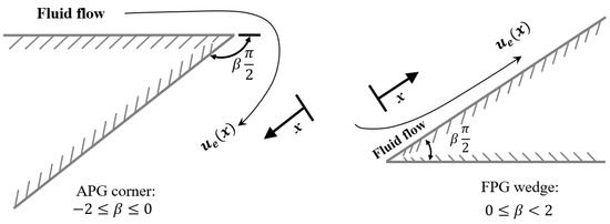
Figure 1.
Falkner–Skan flow schematic, adapted from [3].
We followed Harris et al. [26,27] to non-dimensionalize Equations (1) and (2) by considering the following characteristic length, velocity, and time scales:
where l is a length scale, t is the dimensional time, is the characteristic velocity, is the fluid velocity at the boundary-layer edge, m is the Falkner–Skan power exponent, and is the Reynolds number. Variables , , , , , and are the non-dimensional parallel and perpendicular wall coordinates, the parallel and perpendicular flow velocity components, the velocity at the boundary-layer edge, and the dimensionless time, respectively. Applying dimensionless parameters (6) through (14) to Equations (1) and (2) yields the non-dimensional continuity and x-momentum equations; however, the normalization symbol (*) is dropped for simplicity.
Continuity:
Streamwise x-Momentum Conservation:
- →
- At t = 0, u = 0 and v = 0 for all x and y.
- →
- For t > 0:
- 0, (no-slip condition), u = 0, and v = 0.
- 0, y → ∞, u → .
According to Harris et al. [26,27] the following non-dimensional transformation parameters (mapping) can be applied to the boundary-layer Equations (15) and (16) to perform a transient similarity analysis in such a way as to reduce the number of independent variables from three (u, v, and t) to two ( and ) variables,
where is the reduced stream function; and are the space and time transform variables of similarity, respectively; u and v are the dimensionless parallel and perpendicular components of the fluid flow speed, respectively; x and y are the dimensionless positions parallel and perpendicular to the flow, respectively; and t is the dimensionless time. In order to develop a new similarity solution, the following steps are implemented: (1) Equation (17) is applied to Equation (18) to obtain the normalized flow speed (u), (2) the continuity Equation (15) and the normalized velocity (u) are used to define the normalized v velocity, and (3) the normalized u and v velocities are plugged into Equation (16) as functions of in conjunction with the chain rule for derivatives to finally arrive at the third-order ODE. The reader is referred to [26,27] for a full demonstration.
where f is associated with the flow-stream function, is related to the streamwise fluid velocity, and is related to the local shear stress. As stated before, and are related to space and time, respectively. The corresponding boundary conditions for ≥ 0 are expressed as follows:
Unsteady boundary-layer phenomena can be categorized into two distinct types: start-up processes and shut-down processes [28]. In the context of start-up processes, such as unsteady flows over flat plates, cylinders, and spheres, the flow initiates from a quiescent state (characterized by an inviscid condition), and over time, a transient thin boundary layer develops in proximity to the wall. In contrast, shut-down processes are characterized by the gradual cessation of the flow as time progresses. In the analysis of unsteady flows, the Navier–Stokes equations can be subject to simplifications due to the fact that the time-dependent components of the velocity field are independent of the spatial coordinate (x) parallel to the wall. This reduction results in the governing equation for the unsteady boundary layer flow over a semi-infinite, impulsively started flat plate. Furthermore, it is noteworthy that when variables x, y, and t can be reduced to a single dimensionless variable, a similarity solution for the unsteady boundary layer can be derived.
In this context, several studies [29,30] have investigated the behavior of an incompressible boundary layer over a semi-infinite flat plate that is impulsively initiated from rest with a uniform freestream velocity. The dynamics of this unsteady boundary-layer flow can be categorized into two distinct regimes: the Rayleigh flow regime, which is relevant for small times, and the Blasius flow regime, which corresponds to larger times or the steady-state solution. During the Rayleigh flow phase, the plate is impulsively set into motion, and at a given position (x) from the leading edge, the flow exhibits a square-root dependence on time, indicating that, at these early times, the finiteness of the plate has a negligible effect. In the Blasius flow regime, which corresponds to the longer time or steady-state solution, the flow is assumed to be steady, and at a given x position from the leading edge, the unsteady terms vanish [28,29,30]. Moreover, Harris et al. [26,27] postulated that for short-time solutions (), there exists a transient period during which the effects of the impulsive start are confined to a thin boundary layer adjacent to the surface. The present study focuses on start-up or impulsive flow scenarios. For short-time approximation, the diffusion scale can be expressed as , with the following corresponding variables:
The following prescribed boundary conditions are considered:
According to Harris et al. [26,27] and Schlichting and Gersten [28], for the solution of momentum Equation (16), an ansatz of a power series in is used, yielding the small-time solution for Equation (28):
Applying Equation (32) to Equation (28) yields the following set of momentum equations for the first two terms:
The following boundary conditions are considered:
The approximated transient boundary-layer solution of the normalized skin friction coefficient was calculated by Harris et al. [26,27] as follows:
The normalized boundary-layer thickness is defined as the value of , where the local value of is 0.99. Furthermore, the normalized displacement and momentum thicknesses in Falkner–Skan flows are computed here as in [3]:
Notice that prime denotes differentiation concerning .
3. Solution Strategies for Small Time
This section details the steps used to numerically solve the set of momentum Equations (33) and (34) in terms of , since its boundary conditions are known [9,25]. Rewriting Equations (33) and (34) in terms of yields the following:
Based on a central difference approach (2nd order accurate), the derivatives in Equations (42) and (43) are expressed as follows:
The term can be computed by applying the following forward Euler approach:
Furthermore, the term is calculated by applying a numerical derivative to the term as follows:
Starting node:
Central nodes:
Final node:
A similar procedure is used to obtain the values for the and terms.
In summary, the finite difference strategy for the small-time solution is performed as follows:
- Initialize the and terms.
- Solve Equation (53).
- Solve Equation (50).
- Repeat steps 3 and 4 until the prescribed tolerance is reached.
- Initialize the and terms.
- Solve an equation similar to Equation (53) to obtain the term.
- Solve Equation (51).
- Repeat steps 9 and 10 until the prescribed tolerance is reached.
- Solve Equation (32).
As for steps 5 and 11, a numerical tolerance of is assumed in the calculation truncation (). The iterative error (E) is defined, for instance, as follows:
4. Steady-State Solution
The similarity solution or Falkner–Skan equation [24] for the steady-state boundary-layer equations is expressed as follows:
Boundary Conditions:
where the similarity variable is given as follows:
The Falkner–Skan momentum equation is discretized in terms of via an explicit finite difference scheme as follows:
An explicit method [25] is used to solve Equations (62) and (63). A numerical derivative with a high-order FDM at the corners is used to obtain the terms. The normalized skin friction coefficient for the steady-state case can be defined as in [3,26,27]:
Furthermore, in the Falkner–Skan steady-state solution, the boundary-layer thickness is also defined as the value of , where is 0.999 and the integral boundary-layer parameters (i.e., displacement and momentum thickness) can be found via Equations (40) and (41).
It should be emphasized that the final expression of the Falkner–Skan ODE depends on the setting of the similarity variable (). For example, White [3] defined the similarity variable as follows:
The resulting ODE expression for the Falkner–Skan equation is expressed as follows:
In the present investigation, we utilize the expression in Equation (58) alongside the corresponding similarity variable, as defined in Equation (61), to facilitate a rigorous comparison and validation using the findings of Harris et al. [26,27]. Additionally, Equation (66), in conjunction with the similarity variable (65), is employed and solved to further validate the numerical methodology implemented in this study. This approach is consistent with the work of Simpson [7] and Wazzan et al. [4], who adopted a similar framework to determine the velocity profiles and their respective derivatives, which are subsequently used in stability analysis based on the Orr–Sommerfeld equations.
5. Stability Analysis
This section briefly details the governing equations and boundary/initial conditions for the flow stability analysis. The reader is referred to [3,4,7] for a full demonstration.
In order to perform a linearized stability analysis, a disturbance of the following form is applied to the NS equations:
where , , , and are disturbances in the x, y, and z directions, respectively, and U, V, and W are the velocities in the x, y, and z directions, respectively. Finally, P is the pressure in the x, y, and z coordinates. After applying Equations (68)–(71) to NS, the Navier–Stokes equation yields [3]:
Applying Squire’s [3] theorem, which states that, for a shear parallel flow (), the minimum critical unstable Reynolds number occurs for a two-dimensional disturbance propagating in the same direction, the Orr–Sommerfeld equation is expressed as follows:
where U is the velocity profile of the boundary layer, c is the wave propagation speed, is the disturbance, is the wave number, is the kinematic viscosity, and . In this case, the prime (′) indicates differentiation with respect to y. The Orr–Sommerfeld boundary conditions for external flow are expressed as follows:
Normalizing the Orr–Sommerfeld equation yields the following:
where , , , , , and .
According to Equation (79) and boundary conditions (77) and (78), this is a fourth-order linear, homogenous ODE with zero values at its boundaries, which results in an eigenvalue problem. A temporal stability Orr–Sommerfeld equation is solved via a finite difference scheme with the use of the “eig()” Matlab function to solve for the eigenvalue; additional details are provided in the next section. In summary, FDM is used to discretize the Orr–Sommerfeld equation (Equation (79)), form matrices A and B, finally solving the eigenvalue problem of Equation (97), as described in Section 6.
6. Solution Strategies for Flow Stability Analysis
The Orr–Sommerfeld equation can be solved using a finite difference scheme [7]. Rearranging Equation (79) so that the terms are on the right side and the non- terms are on the left side yields the following:
Equation (87) can be written in matrix form as follows:
where A and B are the left- and right-hand matrices of Equation (87), respectively.
From Equations (87) and (96), it can be seen that A is a pentadiagonal matrix and B is a tridiagonal matrix. In order to solve for the complex value of , Equation (96) yields the following:
This eigenvalue problem can be solved using a Gram–Schmidt algorithm where the matrix (A) is decomposed by the product () of an orthonormal matrix (Q) and an upper triangular matrix (R). Next, a QR matrix algorithm algorithm is applied to obtain the eigenvalues. In this case, the Matlab “eig()” function is used to solve this problem. In order to solve the Orr–Sommerfeld equation, the and in terms of the coordinate must be known. Then, the and are set up. Once this is done, for each value in , the A and B matrices are assembled. Equation (97) is solved using the Matlab “eig()” function, and the most unstable eigenvalue is found and stored at the and coordinates. Finally, neutral stability curves are generated using the MATLAB version R2024b contour plot function, which visualizes the loci of neutral stability in the and parameter space for the temporal stability analysis.
7. Relevant Results and Discussion
This section presents a grid independence test and a thorough validation of the numerical results, with an emphasis on assessing the reliability of the computational approach. The discussion begins with a traditional steady-state analysis () to examine how varying pressure gradients influence certain normalized boundary-layer parameters. In this context, a steady-state analysis is conducted for several distinct pressure gradients, aiming to investigate their impacts on the stability characteristics of the flow. Additionally, the effects of dimensionless time on key flow parameters, including normalized velocity, momentum boundary-layer thickness, displacement thickness, shear stress, and the wall skin friction coefficient, are explored for various pressure gradients. The findings highlight the sensitivity of these parameters to changes in both dimensionless time and the pressure gradient. Furthermore, a stability analysis is performed at a specific strong adverse pressure gradient () of −0.18, examining the flow behavior over a range of dimensionless times. This analysis provides valuable insights into the stability transitions and flow behavior under varying temporal conditions.
7.1. Steady-State Falkner–Skan Flow Parameters
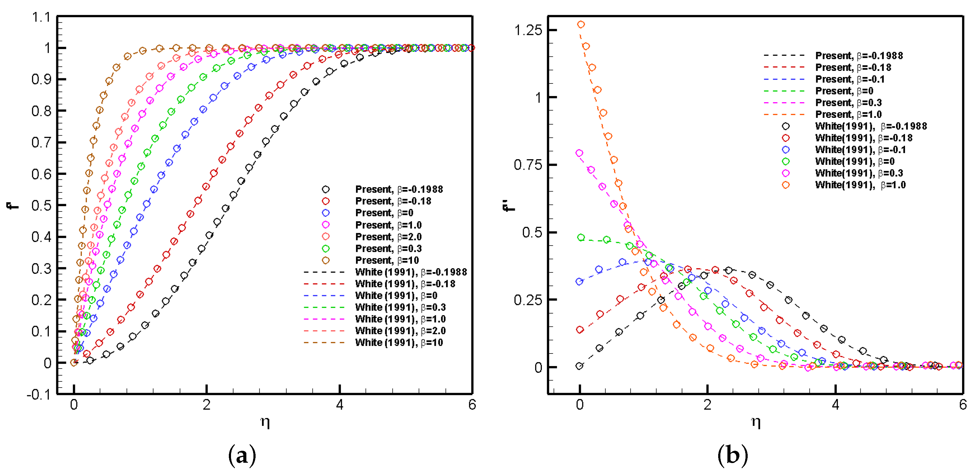
As a special case of the unsteady Falkner–Skan solution, this section discusses the scenario of infinite time, i.e., the steady-state stage. Figure 2a depicts the wall-normal variation of the normalized streamwise fluid velocity () at several pressure gradient strengths of = −0.1988, −0.18, 0, 0.3, 1, 2, and 10. For a fair comparison with White’s results [3], the obtained solutions are based on the dimensionless coordinate of . All curves begin at zero at the wall () due to the non-slip condition and increase until they reach a value of unity in the far field, where the flow velocity matches that of the freestream. As mentioned earlier, the strength and sign of the pressure gradient have a significant impact on the wall velocity gradient and, consequently, on the normalized wall shear stress, or . This topic is further explored in the next figure. It can also be observed that as the pressure gradient increases positively, the streamwise velocity reaches the freestream condition over a short vertical distance from the wall due to the infringed strong flow acceleration, particularly at 10, which means that the boundary-layer thickness shrinks. As the pressure gradient decreases (adverse pressure gradient), the opposite effect is observed: flow retardation is prominent in the near-wall region ( 1) in comparison with the zero-pressure gradient case, and the boundary layer becomes thicker. For very strong APGs, the velocity curves become more “”-shaped, with evident curvature changes or inflection points. The boundary-layer separation or detachment condition is achieved for approximately −0.1988, beyond which the laminar boundary-layer equations can no longer be applied. In comparison to the solution presented by White [3], it is evident from the figure that the two solutions exhibit a high level of agreement across the various pressure gradients.
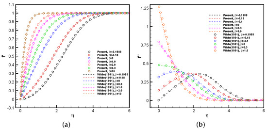
Figure 2.
Steady-state Falkner–Skan solution: (a) solution compared to White’s solution [3]; (b) solution compared to White’ss solution [3].
Figure 2b shows the normalized local shear stress () vs. . The Falkner–Skan solution based on the dimensionless coordinate is . At a zero-pressure gradient ( = 0), or the baseline case, the wall shear stress () is approximately 0.5. Clearly, flow acceleration, or > 0, enhances the wall velocity gradient and, consequently, the local values of the shear stress, particularly in the near-wall region of the boundary layer. No inflection points (i.e., ) are observed for the favorable pressure gradient (FPG) cases, with the exception of the region extending from the boundary-layer edge toward the freestream. This observation suggests that the stabilizing effects of positive values of exert a notable influence on the flow characteristics. Conversely, negative values, or flow deceleration, lead to a retardation of the flow for < 2. Notably, the shear stresses are displaced away from the wall and are predominantly concentrated in the region of 2 < < 4. The presence of local maxima in the profiles signifies the occurrence of singularity points within the flow. The specific value of = −0.1988 corresponds to a critical threshold for flow recirculation, as indicated by the condition of . The results exhibit strong agreement with the findings of White [3]. Table 1 presents the current values for the boundary-layer wall shear stress, displacement thickness, and momentum thickness in comparison with the data provided by White [3] for pressure gradients of −0.19884, −0.18, 0, 0.3, 1, 2, and 10 based on the coordinate of . As observed in Table 1, an increase in the pressure gradient results in a corresponding increase in the wall shear stress, while both the displacement and momentum thicknesses decrease. The displacement and momentum thicknesses are represented by the areas under the curves of (1 − ) and (1 − ), respectively. The area beneath the (1 − ) curve corresponds to the mass flow-rate deficit induced by the no-slip condition and the shear boundary layer, while the area beneath the (1 − ) curve is indicative of the momentum deficit due to viscous forces (drag). The shape factor in the final column, defined as , clearly illustrates the tendency of a large positive pressure gradient to equalize both deficits. Conversely, as the pressure gradient becomes more adverse ( < 0), the flow decelerates more significantly near the wall, leading to more rapid growth of the boundary layer, which substantially affects the growth of the shape factor. Finally, excellent agreement is observed with the numerical results reported by White [3], with the maximum discrepancies found to be within 1–2%.

Table 1.
Present pressure gradient boundary-layer parameters compared to White’s solution [3].
7.2. Temporal Flow Stability Analysis in the Steady-Stage Stage
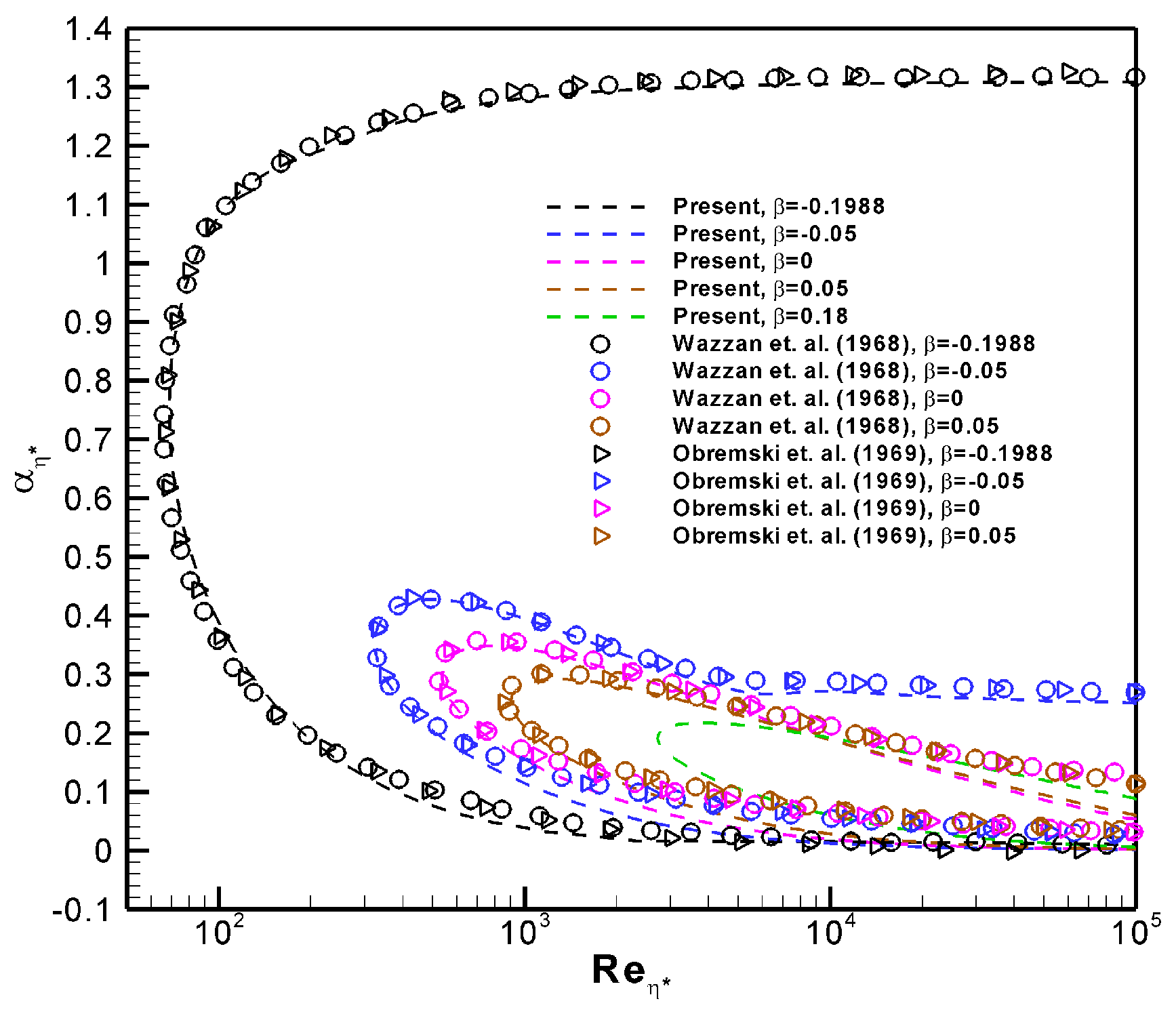
In temporal stability analysis, the focus is on determining whether disturbances (or perturbations) grow or decay over time, which typically leads to the calculation of the critical Reynolds number at which flow becomes unstable, indicating that the disturbances may evolve over time and could lead to the onset of transition to turbulence. On the other hand, spatial stability analysis examines how disturbances grow or decay as they move along the flow direction. Spatial stability analysis can provide different results for critical Reynolds numbers in some cases, but temporal stability is usually the governing analysis for determining when transition occurs. Therefore, the present manuscript focuses on a temporal stability analysis. Figure 3 presents a comparison of the temporal stability results obtained by Wazzan et al. [4] and Obremski et al. [31] under identical pressure gradient parameters () for the respective cases. In general, the agreement is exceptional, further validating the reliability of the present approach. This is particularly evident in the critical region corresponding to the neutral stability curve for Reynolds numbers of interest, specifically in the upper-left region. However, some discrepancies are observed at very high Reynolds numbers (), as our results tend to underpredict the inner unstable region of the neutral curve. These deviations can likely be attributed to the presence of a flat region in the neutral curve. This plateau presents numerical challenges in determining the eigenvalue pair of and . A critical aspect to emphasize is the significant increase in the unstable region due to the presence of a strong separation-induced adverse pressure gradient (APG) at −0.1988. When considering the zero-pressure-gradient (ZPG) flow, or , as the reference case, it is evident that an increase in the pressure gradient () results in a reduction in the maximum dimensionless wavenumber (i.e., or ), accompanied by a rightward shift of the neutral curves. Furthermore, the interior region of the neutral stability curve, corresponding to unstable wavenumber–Reynolds number pairs, contracts, which indicates a stabilizing effect of the favorable pressure gradient on the flow. Specifically, at , the maximum wavenumber associated with the instability is , while at the critical Reynolds number (the leftmost value of ), the wavenumber is ; both values align precisely to those reported by Jordinson [32] and Wazzan et al. [4]. Consequently, the smallest unstable wavelength is or, equivalently, 5.2, based on the current computation of . This suggests that the Tollmien–Schlichting waves exhibit an elongated structure, extending approximately five times the boundary-layer thickness in the streamwise direction [3]. In contrast, for a favorable pressure gradient of , the maximum wavenumber associated with instability decreases to 0.2176, which corresponds to a streamwise wavelength of approximately 8.8 for Tollmien–Schlichting waves in highly accelerated laminar flows. In the context of decelerated flows for , it is evident that the region enclosed by the neutral stability curves (representing the unstable region) experiences a significant expansion, thereby destabilizing the flow. Specifically, for the boundary-layer detachment scenario at , the present results indicate that unstable disturbances are virtually always present for Reynolds numbers exceeding . This observation provides strong evidence that all separation flows in this regime are inherently turbulent. In the case of a very strong adverse pressure gradient (APG), the smallest unstable wavelength is given by , indicating a significant reduction in the minimum wavenumber streamwise length required for the destabilization of the flow through Tollmien–Schlichting waves.
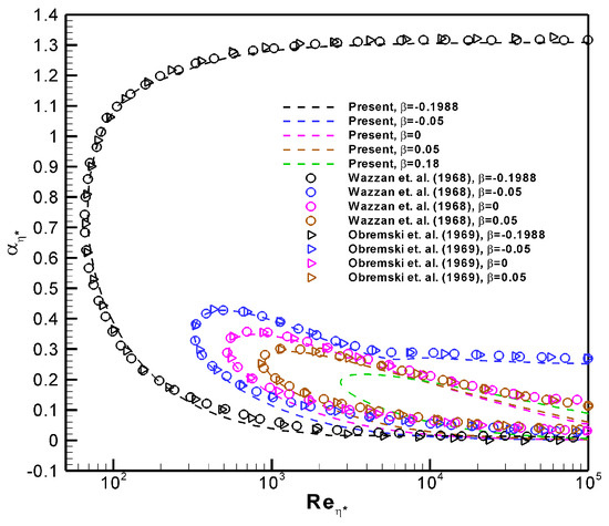
Figure 3.
Steady -state stability for several pressure gradients based on the displacement thickness length scale, in comparison with results reported in [4,31].
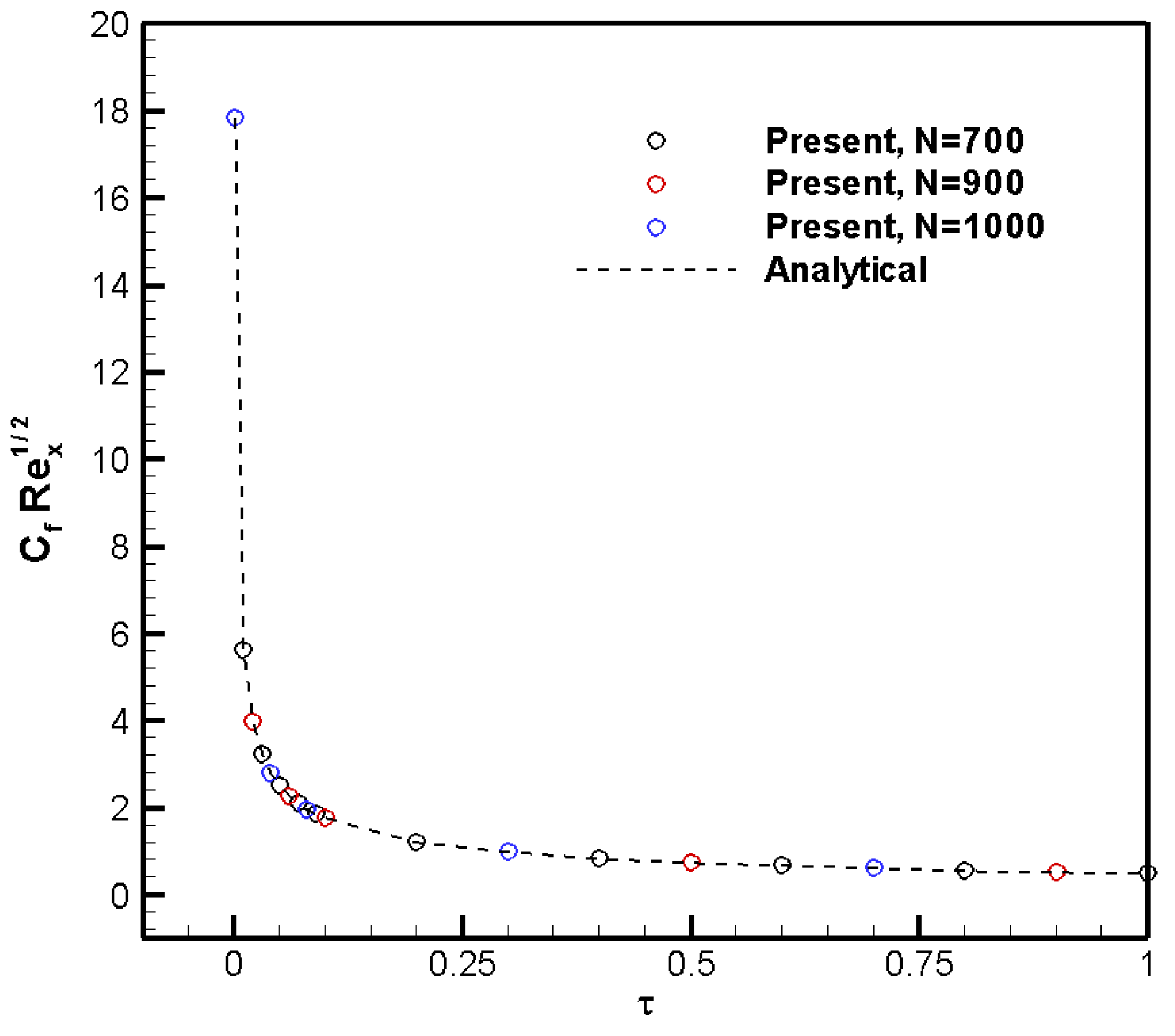
7.3. Grid Independence Test in Unsteady APG Flows
Figure 4 and Table 2 show a grid dependence test comparing the present skin friction coefficient results () at different node numbers (i.e., 700, 900, and 1000) with the analytical expression (Equation (39)) of the skin friction coefficient for a strong adverse pressure gradient (APG) () of −0.18 proposed by [26,27]. In all three cases, the numerical values of almost overlap with the analytical expression. Furthermore, even the “coarse” case with 700 nodes exhibits small discrepancies in the third decimal place (approx. 0.35% of difference) relative to the analytical values, as seen in Table 2, backing the accuracy of our finite difference scheme. However, for better precision, the numerical predictions shown and discussed here are obtained by considering 1000 nodes along the coordinate. In addition, according to Figure 4 and the full data from Table 2, a sharp decline of the initial value of is observed—almost 10 times in barely 0.1 non-dimensional time units () at this pressure gradient ( = −0.18).
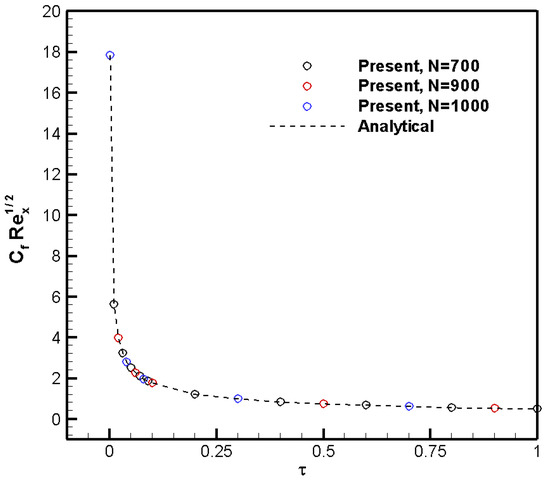
Figure 4.
Grid dependence test for 700, 900, and 1000 nodes at = −0.18.
Table 2.
Temporal variation of the non-dimensional time skin friction coefficient at .
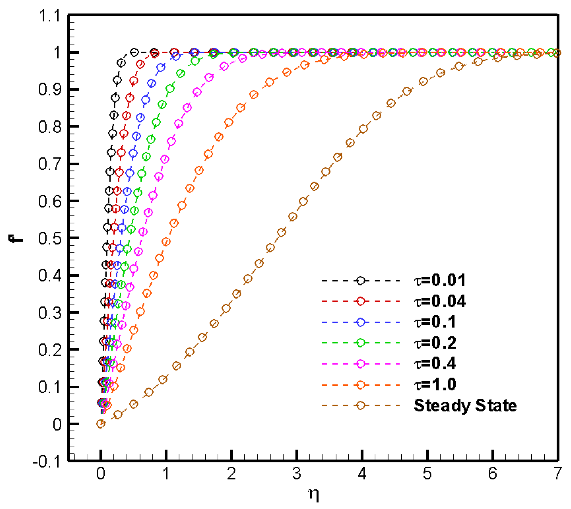
7.4. Transient Analysis of Boundary Layer Parameters
Figure 5 shows the dimensionless velocity function () versus variations at different values and its steady-state solution for a very strong adverse pressure gradient (APG) of −0.18. At 0, the flow field is initialized by the potential freestream velocity. The laminar boundary layer begins to rapidly develop; however, by the unitary non-dimensional time ( 1), the velocity profile does not exhibit any inflection point or curvature change, meaning that the flow is far from the separation flow state. On the other hand, the steady-state solution depicts the typical “S”-shaped profile of strongly decelerated fluid flows [3], with an inflection point where = 0. By comparing with the steady-state solution, we evaluate the flow evolution up to a unitary non-dimensional time ( = 1).
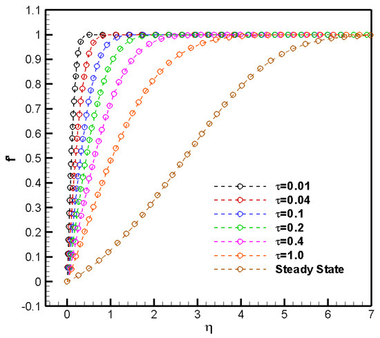
Figure 5.
Dimensionless velocity variation at different non-dimensional times () and −0.18.
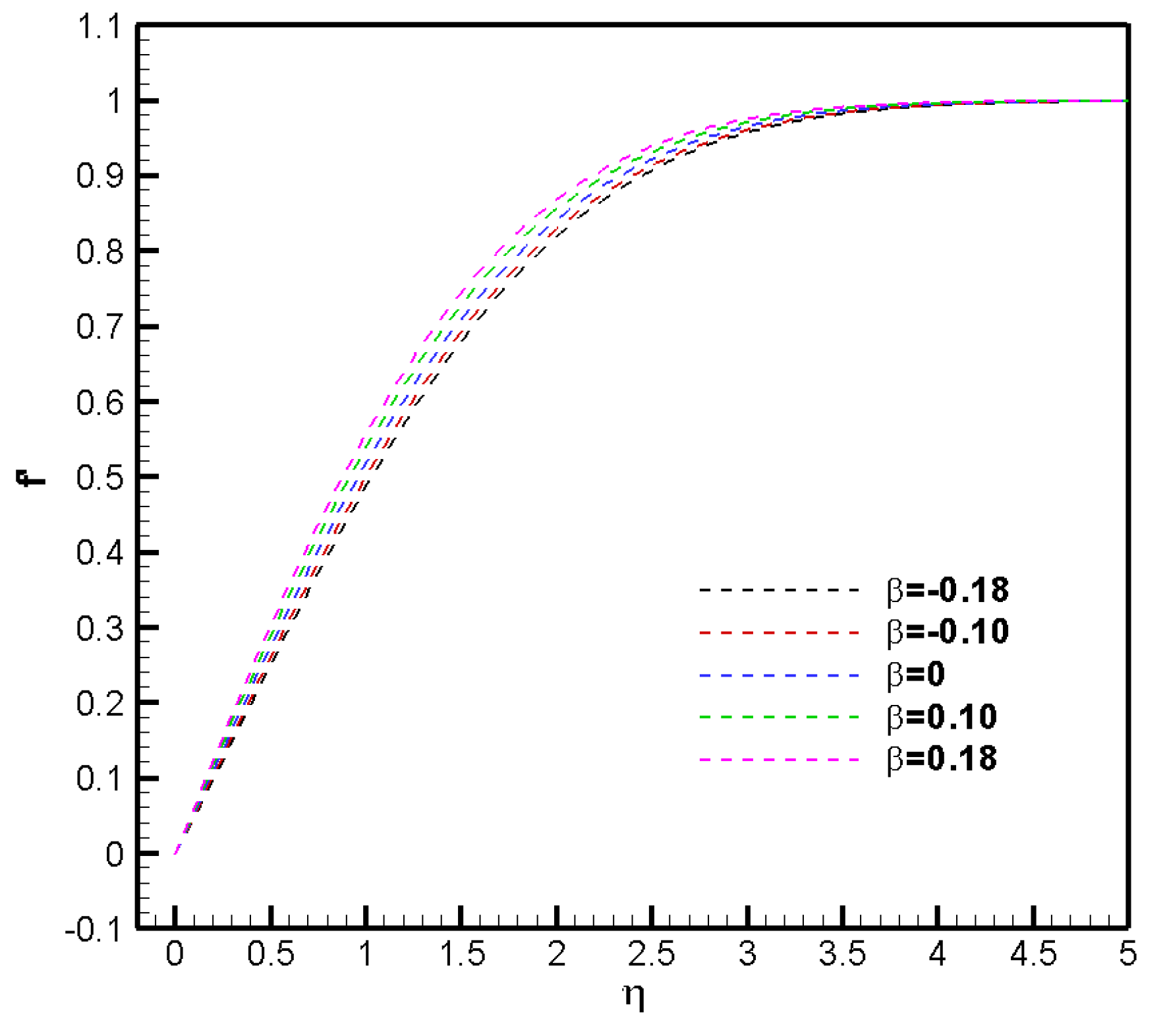
Figure 6 depicts the dimensionless streamwise velocity for different pressure gradients at a dimensionless time () of 1. As the pressure gradient decreases toward negative values (APG), the normalized boundary layer exhibits a thickening process. As mentioned previously, the normalized velocity profile at −0.18 does not exhibit an unstable ‘S’ shape (inflection or singularity point) as in the steady solution shown in Figure 5, indicating that the flow is not susceptible to detachment at this value. It is observed that flow acceleration or favorable pressure gradients (FPG) require a much shorter transient to achieve steady-state conditions, since the developed shear layer is significantly thinner than that of the APG cases. Figure 7a,b illustrate the variation of boundary-layer and displacement thicknesses as a function of the dimensionless time () for pressure gradients of −0.18, −0.10, 0, 0.1, and 0.18. The figures indicate that as increases, both the momentum boundary layer and displacement thicknesses exhibit a corresponding increase, ultimately stabilizing once the system reaches a steady-state condition. Notably, it is observed that as the magnitude of the pressure gradient increases towards FPG values, the boundary-layer and displacement thicknesses are reduced and the system achieved quasi-steady-state conditions more rapidly.
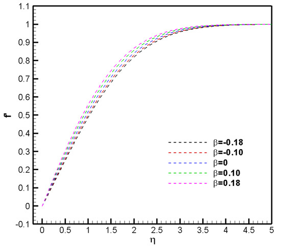
Figure 6.
Dimensionless velocity at = 1 for different pressure gradients ().
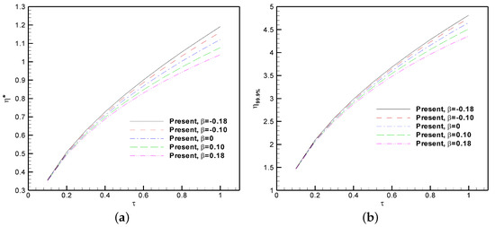
Figure 7.
(a) Momentum boundary-layer thickness () vs. and (b) displacement thickness () vs. for several pressure gradients.
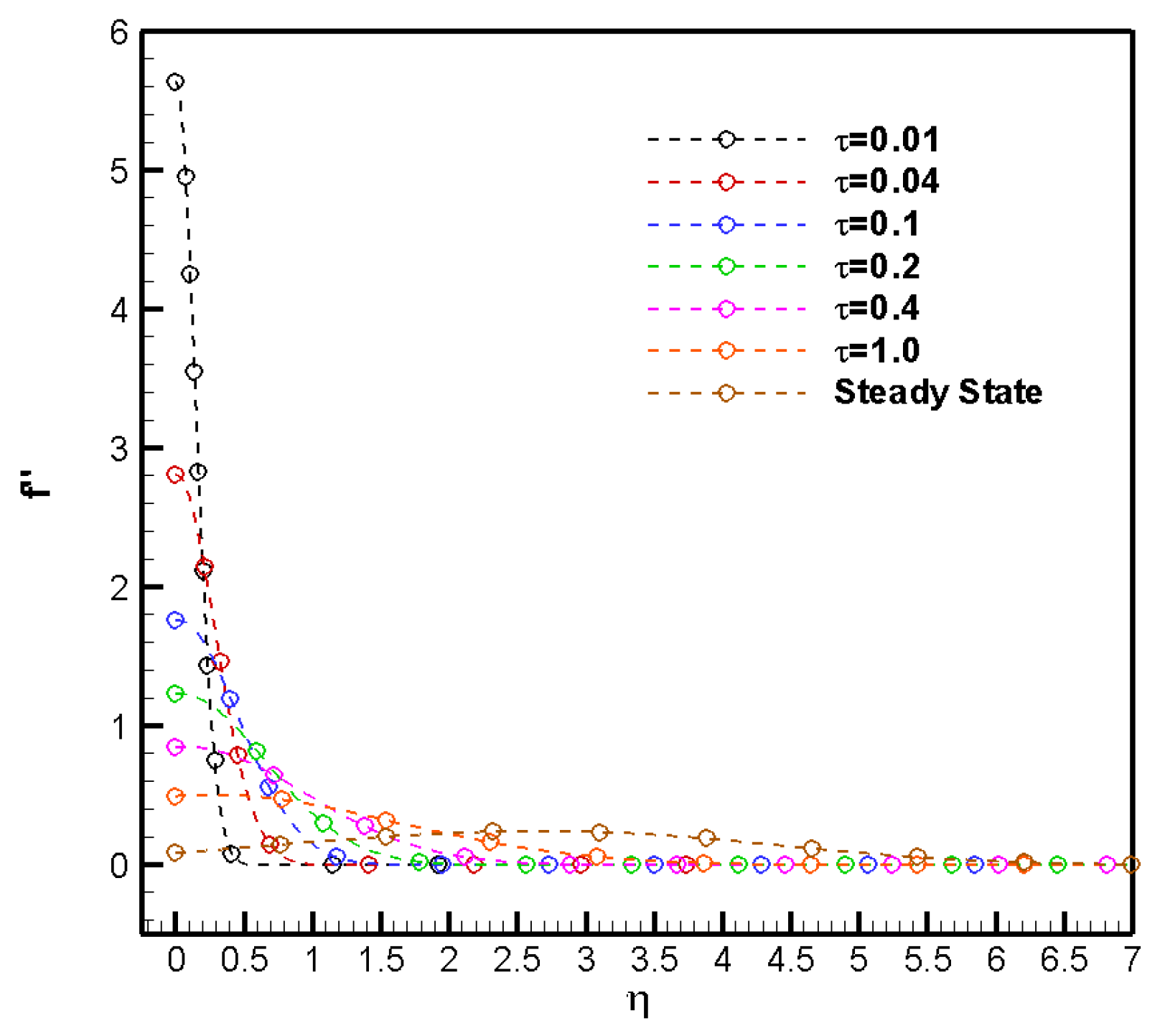
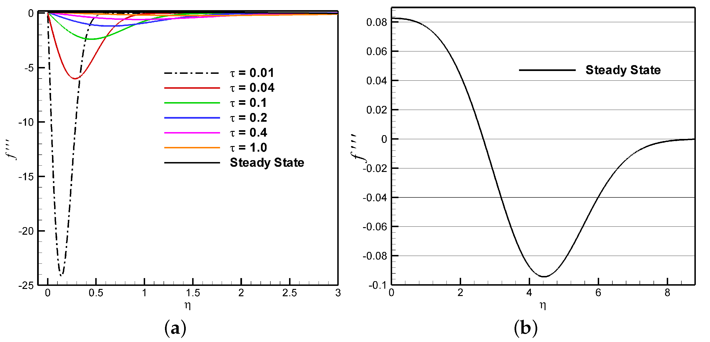
Figure 8 presents the dimensionless shear stress () as a function of the non-dimensional time () for a pressure gradient of −0.18, alongside its corresponding steady-state solution. Initially, large values of can be observed at the wall (i.e., = 0) due to the system’s initialization with freestream values. This results in a pronounced gradient at the wall as the flow transitions from the freestream conditions to the developing boundary layer, reflecting the disparity between the initial and evolving velocity profiles. The data reveal that as increases, the shear stress at the wall progressively decreases, eventually stabilizing under the steady-state condition. Notably, for a strong adverse pressure gradient of = −0.18, the shear stress at = 1 is observed to be significantly distant from the steady-state value, indicating that the system has not yet reached equilibrium at this unitary time in the near-wall region (0 ). In a similar manner, the third derivative of the similarity variable (f) is computed and analyzed to evaluate the presence of potential singularity points. In a fluid flow velocity profile, an “inflection point” refers to a specific boundary-layer location where the curvature of the velocity profile undergoes a change. This point marks a transition in the rate of change of velocity with respect to distance: the behavior shifts from an increasing to a decreasing rate of change (or vice-versa). Essentially, it signifies a change in the curvature of the flow profile. Inflection points are often associated with flow instabilities, as they are linked to the presence of strong shear forces at that location, which may facilitate the onset of transition or flow separation. In Figure 9a, the normalized second derivative of the fluid velocity () is plotted at different values for −0.18. Peaks of shrink and move farther from the wall during the transient stage. No inflection points (i.e., ) are observed for 1, except for the steady-state profile. A detailed view of the third derivative in the steady state is shown in Figure 9b, where an inflection point () is identified at 2.6. This observation is consistently supported by the presence of a local maximum in at the corresponding wall-normal location in Figure 8, which aligns with theoretical predictions.
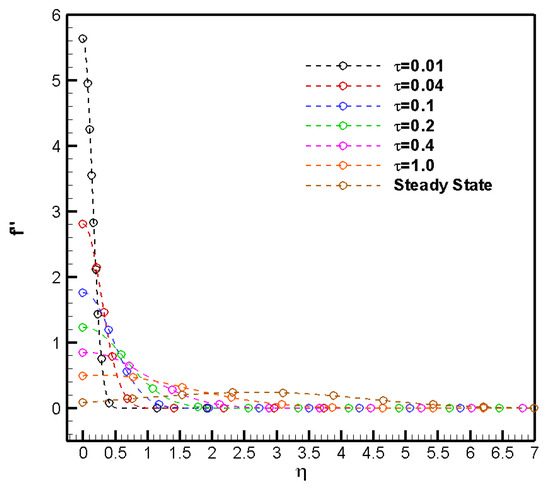
Figure 8.
Dimensionless shear stress () at different values for −0.18.
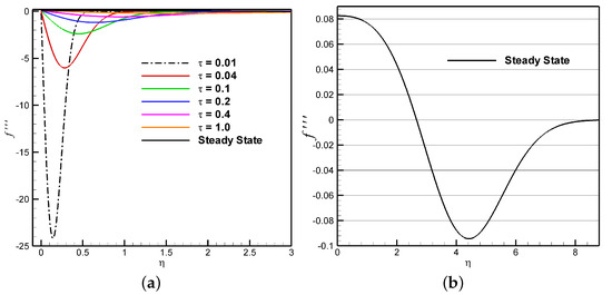
Figure 9.
Normalized second derivative of the fluid velocity () at −0.18: (a) at different values; (b) close-up of the steady-state profile.
Figure 10a illustrates the non-dimensional shear stress () for various pressure gradients at a dimensionless time of = 1. As expected, the figure reveals that as the pressure gradient increases, the shear stress at the wall (i.e., ) also increases. Interestingly, a significant collapse of all profiles is observed, starting from 1 and extending towards the edge of the momentum boundary layer. This behavior corroborates the observation that the majority of the flow changes occur within the innermost 20–25% of the boundary-layer region, closest to the wall. Even in the case of a very strong adverse pressure gradient (APG) with = −0.18, the wall shear stress exhibits relatively large values, indicating that at this unitary value of , the boundary layer is neither prone to detachment nor close to reaching its steady-state condition. Figure 10b depicts the temporal evolution of the normalized skin friction coefficient for pressure gradients of −0.18, −0.1, 0 (ZPG), 0.1, and 0.18 compared to the trend line provided in Table 3. Sharp decreases in the parameters are observed within the unitary time scale, with reductions ranging from 2.8× to 4×, depending on the prescribed non-dimensional pressure gradient. Flows characterized by negative values, indicative of decelerated flow conditions, exhibit more pronounced and steeper decreases in comparison to other cases. Finally, the power-law trend lines closely align with the current numerical predictions, suggesting that this approximation can serve as a reliable method for estimating the temporal evolution of the skin friction coefficient in unsteady problems.
Figure 10.
(a) Dimensionless shear stress at a of 1 and (b) the wall skin friction coefficient for several pressure gradients.
Table 3.
Trendline equation parameters.
7.5. Temporal Flow Stability Analysis in the Transient Stage
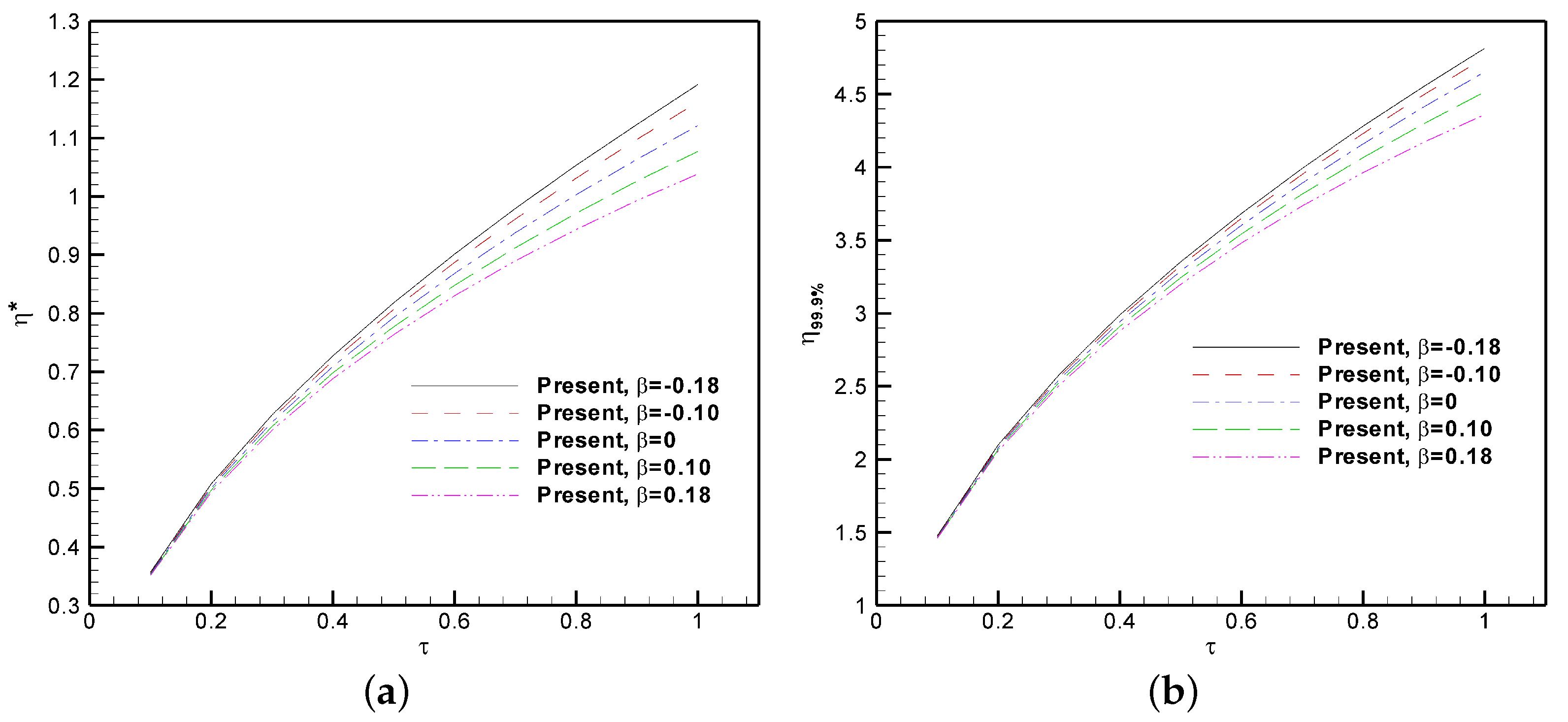
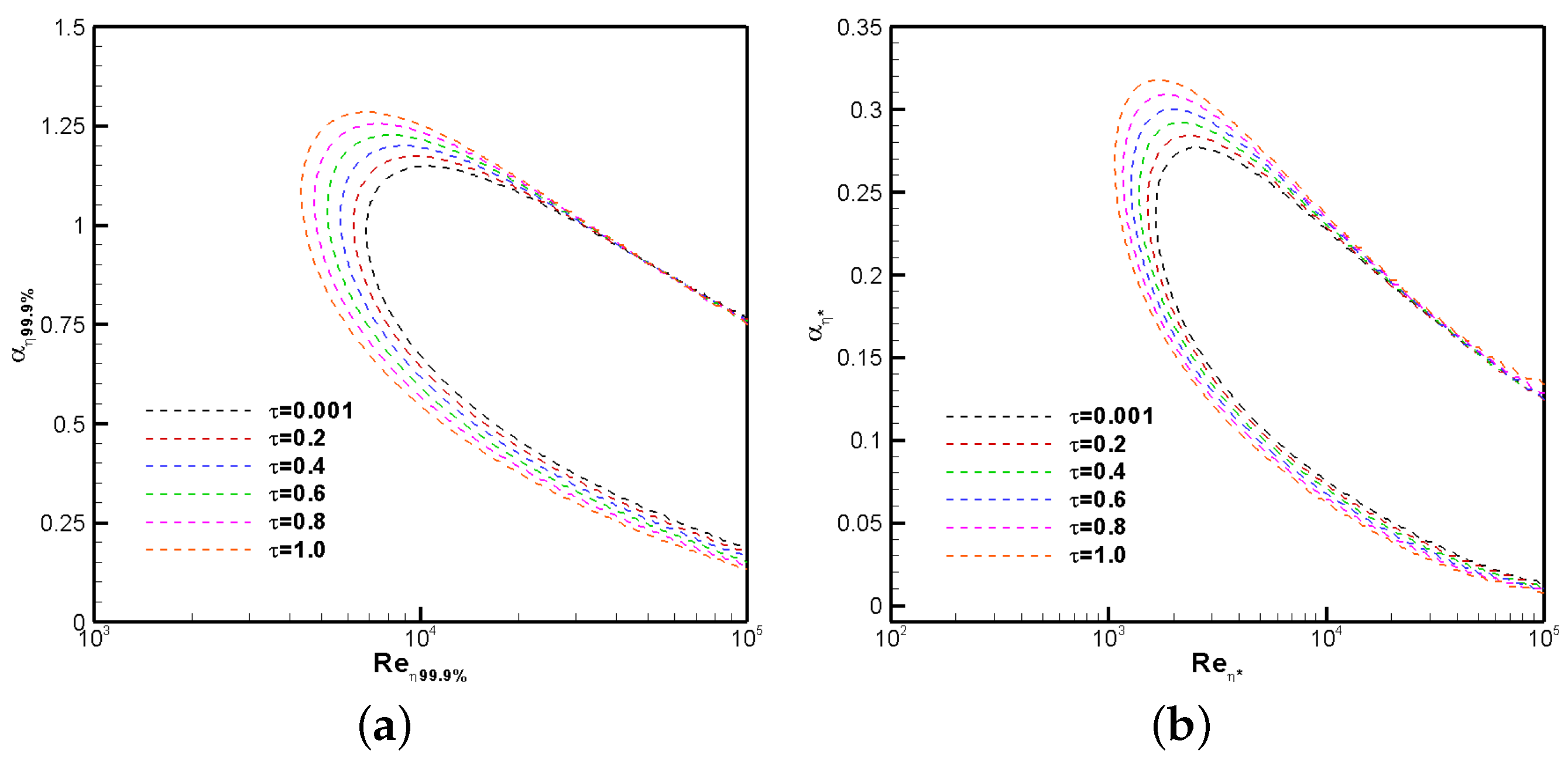
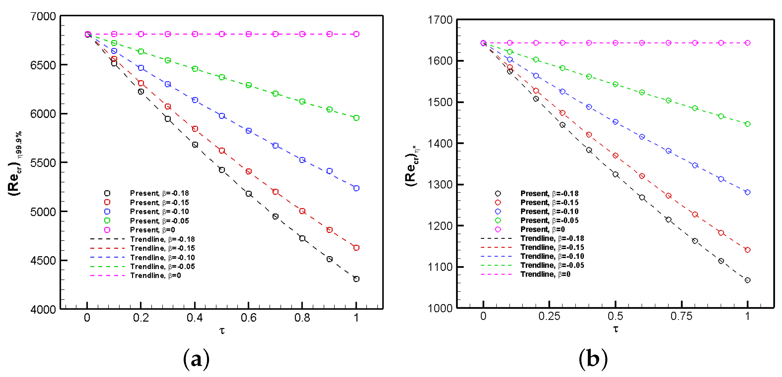
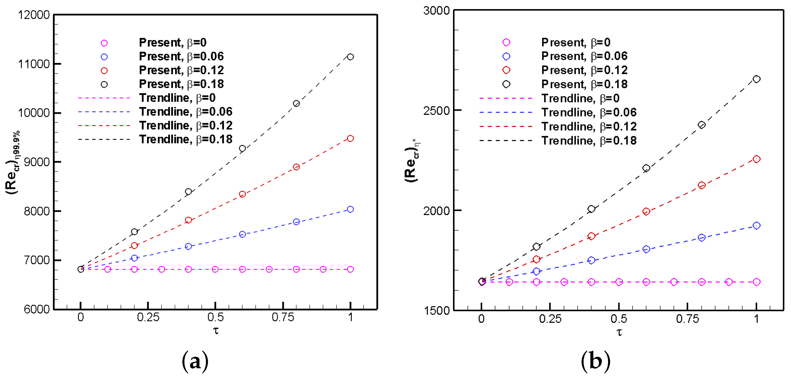
Figure 11a,b show the neutral stability curves for different values (i.e., 0.001, 0.2, 0.4, 0.6, 0.8, and 1.0) at a pressure gradient of −0.18 based on length scales of and , respectively. Here, is the dimensionless momentum boundary-layer thickness based on of the freestream velocity, whereas is the dimensionless displacement thickness. In temporal flow stability analysis, the neutral curve is described by zero values of (normalized speed propagation of disturbances) and represents a line on a graph that separates the stable flow region (outer) from the unstable flow region (inner). Any flow perturbation occurring within the neutral curve, corresponding to a specific combination of Reynolds number, Re, and wavenumber (), exhibits neither amplification nor attenuation. It can be seen in Figure 11a,b that the inflection points of the neutral curves (i.e., ∂ 0 or ∂ 0 in Figure 11b) move to the left (at lower critical Reynolds numbers) as the non-dimensional time () increases until it reaches its steady-state condition. Furthermore, the inner areas (i.e., the unstable region) become larger with increasing time. Consequently, the flow becomes increasingly susceptible to instabilities during the transient phase, facilitating the emergence of Tollmien–Schlichting waves. The presence of these waves serves as a definitive indicator of the onset of transition, signifying the transition from laminar to turbulent flow behavior. These instabilities manifest as localized disturbances that grow in amplitude, marking a critical stage in the transition process. Figure 12a,b depict the critical Reynolds numbers for different times based on different length scales—the momentum boundary layer and displacement thickness coordinates—and several pressure gradients (). It is important to note that the thickness of the velocity boundary layer is defined as the value of where the local normalized streamwise velocity (u) reaches of the edge velocity () (i.e., = 0.999). In both figures, nearly linear decreasing trends in time are observed at the different values, with steeper decreases for stronger APGs (i.e., for −0.18). The pressure forces cause significant flow deceleration in the near-wall region, which leads to the formation of inflection points, making the flow more susceptible to instability. As the adverse pressure gradient decreases, the critical Reynolds number curves flatten, with a very low decreasing rate for the flat-plate boundary-layer case ( 0). The trendline curves in Figure 12a,b are based on power-law curve fittings, as seen in Table 4, faithfully representing the temporal variation of the critical Reynolds numbers subject to different flow deceleration regimes. The effects of the favorable pressure gradient (FPG) on the transient critical Reynolds numbers are depicted by Figure 13a,b, taking and , respectively, as length scales. Unlike APG trends, the application of flow acceleration or FPGs clearly stabilizes the laminar flow by increasing the critical Reynolds numbers () during the initial transient stage. Similar conclusions were reported by [4] for accelerated flows under steady-state conditions. The rate of change of with time becomes more pronounced at higher FPG strengths. The exponents corresponding to the power-law curve fitting are presented in Table 5, which effectively capture the temporal variation of the critical Reynolds numbers with varying FPGs. The computed value for under the steady-state condition is approximately 3500 at = 0.18. Based on the power-law function, this value is reached at 1.6, indicating a very short transient time in highly accelerated laminar flows.
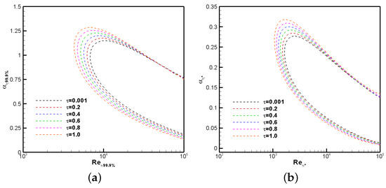
Figure 11.
Transient stability analysis for a pressure gradient of −0.18 based on the (a) boundary-layer thickness coordinate and (b) displacement thickness coordinate.
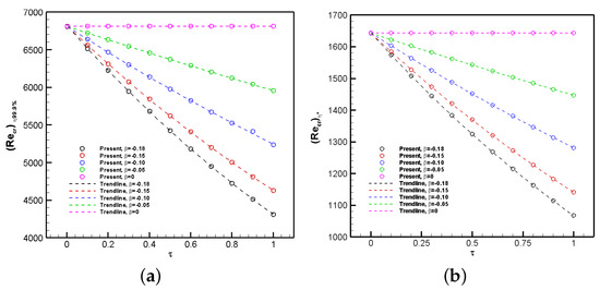
Figure 12.
Transient critical Reynolds number analysis for several adverse pressure gradients based on the (a) boundary-layer thickness coordinate and (b) displacement thickness coordinate.
Table 4.
Trendline and equation parameters for adverse pressure gradients.
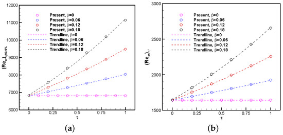
Figure 13.
Transient critical Reynolds number analysis for several favorable pressure gradients based on the (a) boundary-layer thickness coordinate and (b) displacement thickness coordinate.
Table 5.
Trendline and equation parameters for favorable pressure gradients.
The most significant observed behavior is the rapid response of positive values (FPG) in achieving the steady-state critical Reynolds numbers (approximately 1). In contrast, flows with an adverse pressure gradient (APG) or 0 exhibit a much slower response. For example, at = −0.18, the flow requires approximately 6.8 to reach the steady-state critical Reynolds number.
8. Conclusions
The transient and steady-state solutions of the laminar boundary-layer equations subject to streamwise pressure gradients (Falkner–Skan or wedge flows) were solved effectively using an explicit finite difference scheme. The zero-pressure-gradient case, specifically the Blasius solution over a flat plate, was also examined. Furthermore, a stability analysis was performed using a finite difference discretization in conjunction with the Matlab “eig()” function to solve Equation (79). In this case, an optimum number of 1000 nodes was chosen to achieve good precision.
For steady-state flow, it has been observed that positive values of the pressure gradient parameter () exert a stabilizing effect on the flow characteristics. Conversely, negative values of , corresponding to flow deceleration, result in the retardation of the flow for < 2. Notably, under these conditions, the shear stresses are displaced away from the wall and are predominantly concentrated within the region of 2 < < 4. In terms of temporal flow stability, the strength of the pressure gradient significantly influences the streamwise extent of the Tollmien–Schlichting (TS) waves. For zero-pressure-gradient (ZPG) flows, the streamwise length of these instability waves extends approximately five times the boundary-layer thickness. In contrast, for a favorable pressure gradient of , the maximum wavenumber associated with instability is reduced to 0.2176. This corresponds to a streamwise wavelength of approximately 8.8, indicating that the Tollmien–Schlichting waves are considerably elongated in highly accelerated laminar flows. In the case of a very strong adverse pressure gradient (APG), the minimum unstable wavelength is given by , which demonstrates a significant reduction in the streamwise length of the smallest unstable wavelength required to destabilize the flow via Tollmien–Schlichting waves. This reduction signifies that the destabilization of the flow occurs over a much shorter streamwise distance under the influence of a strong adverse pressure gradient. It has been observed flow acceleration and favorable pressure gradients (FPGs) result in a much shorter transient time to reach steady-state conditions, as the developed shear layer is significantly thinner compared to cases with adverse pressure gradients (APGs). During the transient stage (i.e., for 1), the majority of the flow modifications occur within the innermost 20–25% of the boundary layer, closest to the wall. For unitary dimensionless time, the neutral curves in the temporal stability analysis shift towards higher Reynolds numbers (indicating more stable conditions) when positive values of are applied. Conversely, when negative values of or flow deceleration are considered, the neutral curves shift to the left, signifying destabilizing flow conditions relative to the initial state. The most notable outcome is the time response required to reach the steady-state critical Reynolds numbers: approximately 1 for = 0.18 (FPG) and 6.8 for = −0.18 (APG).
With respect to future work, we envision incorporating the effects of wall curvature into the transient stability analysis of Falkner-Skan flows [33].
Author Contributions
Conceptualization, G.A. and M.R.; methodology, G.A. and M.R.; software, G.A. and M.R.; validation, G.A. and M.R.; formal analysis, G.A. and M.R.; investigation, G.A. and M.R.; resources, G.A.; data curation, M.R.; writing—original draft preparation, G.A.; writing—review and editing, G.A. and M.R.; visualization, G.A. and M.R.; supervision, G.A.; project administration, G.A.; funding acquisition, G.A. All authors have read and agreed to the published version of the manuscript.
Funding
This material is based upon work supported by the National Science Foundation under Grant No. 2314303.
Institutional Review Board Statement
Not applicable.
Informed Consent Statement
Not applicable.
Data Availability Statement
Data are contained within the article.
Acknowledgments
The insightful comments from reviewers on this manuscript are greatly appreciated, as they significantly improved its quality.
Conflicts of Interest
The authors declare no conflicts of interest.
Abbreviations
| APG | Adverse Pressure Gradient |
| Crit | Critical |
| DNS | Direct Numerical Simulation |
| FDM | Finite Difference Method |
| FPG | Favorable Pressure Gradient |
| FS | Falkner-Skan |
| NPSE | Nonlinear Parabolized Stability Equations |
| NS | Navier–Stokes |
| ODE | Ordinary Differential Equations |
| OSE | Orr–Sommerfeld Equations |
| PDE | Partial Differential Equations |
| POD | Proper Orthogonal Decomposition |
| TS | Tollmien-Schilchting |
| ZPG | Zero Pressure Gradient |
| 2D | Two-Dimensional |
References
- Clay Mathematics Institute. Navier-Stokes Equation. Available online: https://www.claymath.org/millennium/navier-stokes-equation/ (accessed on 1 February 2025).
- Çengel, Y.A.; Cimbala, J.M. Fluid Mechanics Fundamentals and Applications, 3rd ed.; McGraw-Hill: New York, NY, USA, 2014. [Google Scholar]
- White, F.M. Viscous Fluid Flow; McGraw-Hill: New York, NY, USA, 1991. [Google Scholar]
- Wazzan, A.R.; Okamura, T.; Smith, A.M.O. Spatial and Temporal Stability Charts for the Falkner-Skan Boundary Layer Profiles; REPORT DAC-67086; DOUGLAS AIRCRAFT COMPANY: Springfield, VA, USA, 1968. [Google Scholar]
- Schubauer, G.; Skramstad, H.K. Laminar-boundary-layer oscillations and transition on a flat plate. J. Res. Natl. Bur. Stand. 1947, 38, 251. [Google Scholar]
- Ishak, A.; Nazar, R.; Pop, I. Falkner-Skan Equation for Flow Past a Moving Wedge with Suction or Injection. J. Appl. Math. Comput. 2007, 25, 67–83. [Google Scholar]
- Simpson, C. Temporal and Spatial Stability Analysis of the Orr-Sommerfeld Equation. 2015. Available online: https://www.cdsimpson.net/2015/04/temporal-and-spatial-stability-analysis.html (accessed on 5 February 2025).
- Banks, W.H.H.; Drazin, P.G. Perturbation Methods in Boundary-Layer Theory. J. Fluid Mech. 1973, 58, 763–775. [Google Scholar]
- Han, S. Finite difference solution of the Falkner-Skan wedge flow equation. Int. J. Mech. Eng. Educ. 2013, 41, 1–7. [Google Scholar]
- Wazzan, A.R.; Okamura, T.; Smith, A.M.O. The Stability of Water Flow over Heated and Cooled Flat Plates. J. Heat Transfer. 1968, 90, 109–114. [Google Scholar]
- Govindarajan, R.; Narashima, R. Stability of spatially developing boundary layers in pressure gradients. J. Fluid Mech. 1995, 300, 117–147. [Google Scholar]
- Bertolotti, F.P.; Herbert, T.; Spalart, P. Linear and nonlinear stability of the Blasius boundary layer. J. Fluid Mech. 1992, 242, 441–474. [Google Scholar]
- Saric, W.S.; Reed, H.L.; White, E.B. Stability and transition of three-dimensional boundary layers. Annu. Rev. Fluid Mech. 2003, 35, 413–440. [Google Scholar]
- Perez, J.M.; Rodirguez, D.; Theofilis, V. Linear global instability of non-orthogonal incompressible swept attachement-line boundary layer flow. J. Fluid Mech. 2012, 710, 131–153. [Google Scholar]
- Wazzan, A.; Taghavi, H.; Keltner, G. Effect of boundary-layer growth on stability of incompressible flat plate boundary layer with pressure gradient. Phys. Fluids 1974, 17, 1655–1660. [Google Scholar]
- Maslowe, S.A.; Spiteri, R.J. The continuous spectrum for a boundary layer in a streamwise pressure gradient. Phys. Fluids 2001, 13, 1294–1299. [Google Scholar]
- Jordinson, R. Spectrum of Eigenvalues of the Orr Sommerfeld Equation for Blasius Flow. Phys. Fluids 1971, 14, 2535–2537. [Google Scholar]
- Stewartson, K. The Theory of Unsteady Boundary Layers. In Advances in Applied Mechanics; Academic Press: New York, NY, USA, 1960; Volume 6, pp. 1–37. [Google Scholar]
- Stewartson, K. On the Impulsive Motion of a Flat Plate in a Viscous Fluid II; Department of Mathematics, University College: London, UK, 1972; pp. 143–152. [Google Scholar]
- Riley, N. Unsteady laminar boundary layers. Siam Rev. 1975, 17, 274–297. [Google Scholar]
- Hall, M. A numerical method for calculating unsteady two-dimensional laminar boundary layers. Ingenieur-Archiv 1969, 38, 97–106. [Google Scholar]
- Nanbu, K. Unsteady Falkner-Skan Flow; Institute of High Speed Mechanics, Tohoku University: Sendai, Japan, 1971; Volume 22, pp. 1167–1172. [Google Scholar]
- Blasius, H. Grenzschichten in Flüssigkeiten mit kleiner Reibung. Z. Angew. Math. Phys. 1908, 56, 1–37. [Google Scholar]
- Falkner, V.; Skan, S. LXXXV. Solutions of the boundary-layer equations. Lond. Edinb. Dublin Philos. Mag. J. Sci. 1931, 12, 865–896. [Google Scholar] [CrossRef]
- Pletcher, R.H.; Tannehill, J.C.; Anderson, D.A. Computational Fluid Mechanics and Heat Transfer; CRC Press: Boca Raton, FL, USA, 2013. [Google Scholar]
- Harris, S.D.; Ingham, D.B.; Pop, I. Unsteady Heat Transfer in Impulsive Falkner-Skan Flows: Constant Wall Heat Flux Case. Acta Mech 2008, 201, 185–196. [Google Scholar]
- Harris, S.D.; Ingham, D.B.; Pop, I. Unsteady Heat Transfer in Impulsive Falkner-Skan Flows: Constant Wall Temperature Case. Eur. J. Mech. B/Fluids 2002, 21, 447–468. [Google Scholar]
- Schlichting, H.; Gersten, K. Boundary-Layer Theory; Springer: Berlin/Heidelberg, Germany, 2017. [Google Scholar]
- Hall, M. The boundary-layer over an impulsively started flat plate. Proc. Royal Soc. A London 1969, 310, 401–414. [Google Scholar]
- Smith, S. The impulsive motion of a wedge in a viscous fluid. J. Appl. Math. Phys. (ZAMP) 1967, 18, 508–522. [Google Scholar]
- Obremski, H.J.; Morkovin, M.V.; Landahl, M. A portfolio of stability characteristics of incompressible boundary layers. AGARD-OGRAPH-134 1969, 400043, 1–128. [Google Scholar]
- Jordinson, R. The flat plate boundary layer. Part 1. Numerical integration of the Orr–-Sommerfeld equation. J. Fluid Mech. 1970, 43, 801–811. [Google Scholar] [CrossRef]
- Ramirez, M.; Araya, G. Falkner-Skan Similarity Flow Solutions Subject to Wall Curvature and Passive Scalar Transport. In Proceedings of the 7th Thermal and Fluids Engineering Conference (TFEC2022), Las Vegas, NV, USA, 15–18 May 2022. [Google Scholar]


Disclaimer/Publisher’s Note: The statements, opinions and data contained in all publications are solely those of the individual author(s) and contributor(s) and not of MDPI and/or the editor(s). MDPI and/or the editor(s) disclaim responsibility for any injury to people or property resulting from any ideas, methods, instructions or products referred to in the content. |
© 2025 by the authors. Licensee MDPI, Basel, Switzerland. This article is an open access article distributed under the terms and conditions of the Creative Commons Attribution (CC BY) license (https://creativecommons.org/licenses/by/4.0/).