Abstract
For an extended lattice Boltzmann model based on a product-form equilibrium distribution function, an improved regularization model with enhanced numerical stability is proposed. In this paper’s regularized collision model, coefficients are calculated using two distinct methods during the reconstruction of the non-equilibrium distribution. The first method stems from the direct projection of the non-equilibrium distribution, while the second method relies on the regularization step, which is refined through the recursive calculation of the coefficients of non-equilibrium Hermite polynomials. Compared to the original lattice Boltzmann model, the recursive regularization method significantly enhances the stability of the numerical scheme by appropriately filtering out second-order and/or higher-order non-hydrodynamic contributions. Initially, under isothermal conditions, the periodic double-shear layer simulations are conducted at Reynolds numbers ranging from 104 to 106, testing the enhanced effect of the regularized model in broadening its available speed range. Subsequently, with a fixed Reynolds number, simulations are performed at various temperature values to assess the model’s performance when deviating from the lattice reference temperature. The results demonstrate that, compared to the original model, the recursive regularization model exhibits improved stability and widens the model’s usable speed and temperature ranges.
1. Introduction
Over the past few decades, the lattice Boltzmann method (LBM), as a kinetic theory method based on the discrete Boltzmann equation, has garnered widespread attention in computational fluid dynamics (CFD). LBM has proven to be an attractive and effective tool for simulating complex fluid flows and has been applied to a wide range of fluid dynamics problems, including but not limited to turbulence [1], multiphase flows [2,3], reactive flows [4], nanoscale flows [5], nuclear reactors [6], acoustics flows [7], and thermal flows [8,9]. Compared to traditional CFD methods, the advantage of the LBM lies in the simplicity and locality of its fundamental numerical algorithm, which can be summarized into two parts: the streaming process along discrete velocities and the collision-equilibration process at local location [10,11]. However, it is well known that the LBM faces significant challenges when dealing with high-speed flows, and its success is mainly limited to low-speed incompressible flow applications.
When using the LBM on a standard lattice template to recover the Navier–Stokes (NS) equation under the hydrodynamic limit, there is an error term related to the Galilean invariance in the stress tensor, which can be neglected only when the velocity approaches zero and the flow field temperature is taken as the lattice reference temperature [12]. This hinders the development of the LBM towards higher velocity application scenarios and also limits its application in simulating physical phenomena with variable temperatures. Therefore, for thermal flow problems with large Reynolds numbers, it is necessary to consider eliminating the impact of these errors when using LBM solvers for numerical simulation. A natural method to overcome this limitation is to include more discrete velocities and use an allowable high-order (or multi-velocity) lattice template to ensure Galilean invariance and temperature independence of the stress tensor [13,14,15]. Although models based on high-order lattices have successfully simulated compressible flows to some extent, they not only increase the computational workload but are also limited by the temperature range [16,17].
Another method maintains the simplicity and computational efficiency of the standard lattice and employs a correction term to eliminate the aforementioned error terms in the stress tensor. This method has received widespread attention in recent years [18,19]. Due to the inherent non-uniformity of the correction term, there are different implementations in the literature, all of which recover the same equations in the hydrodynamic limit [20,21,22]. For a detailed overview of different implementations, please refer to the work of Hosseini et al. [23].
Computational stability is crucial for an effective lattice Boltzmann method. If the collision and stream algorithms of the LBM remain unchanged, one of the few key factors affecting the stability of the numerical method is the specific form of the collision operator. The Bhatnagar–Gross–Krook (BGK)-type collision operator has some drawbacks in the application of the LBM, such as numerical instability under high Reynolds numbers and limitations imposed by the Prandtl number in thermal flow calculations. When the Mach number and temperature fluctuations increase, the LBM-BGK scheme may also exhibit numerical instability. Some researchers attribute these instabilities to non-hydrodynamic modes [24], which are non-physical waves contained in the discrete-velocity Boltzmann equation and fall outside the scope of the Navier–Stokes equation [25].
To enhance numerical stability, various collision operators have been proposed, including the multiple relaxation time operator [26]. The so-called multiple relaxation time collision operator involves using different relaxation time factors for each macroscopic moment, thereby stabilizing the computation. Regularized collision operators represent another approach that can filter out contributions from non-hydrodynamic modes [27] to improve numerical stability. There are three primary forms of regularization methods: projection-based regularization [28], recursive regularization [29], and hybrid recursive regularization collision operators [30]. The primary distinction among these three methods lies in the reconstruction approach of the expansion coefficients of the non-equilibrium distribution function.
An extended equilibrium distribution function scheme is proposed in paper [31], which can restore Galilean invariance and satisfy the isotropy of the stress tensor by adding an extension term. This correction method extends the lattice Boltzmann model to simulations with higher flow velocity and can be used in situations deviating from the lattice reference temperature, thus enabling the calculation of thermal flow problems with significant temperature differences. Additionally, the extended model is also applicable to stretched lattices, which are useful when the flow gradient dominates in one direction. However, our numerical tests reveal that the model in paper [31] encounters a narrowing of the usable temperature and velocity range at higher Reynolds numbers. In this paper, we further improve this thermally compressible model using a regularization reconstruction method. The improved model is tested through benchmark examples of plane shear wave decay and periodic double-shear flow. The results indicate that the improved model exhibits a broader computational stable range compared to the original model, both at the lattice reference temperature and in situations deviating from it.
The remaining part of this paper is organized as follows: Section 2 first presents the details of the thermally compressible LBM and the corresponding calculation method for the equilibrium distribution function. Then, it introduces the regularized reconstruction process of the LBM and the calculation method for the corresponding non-equilibrium distribution function. In Section 3, through benchmark test cases, the decay of a plane shear wave and a double-shear flow case, the Galilean invariance, isotropy, temperature independence, and numerical stability of the model are verified and analyzed. The conclusion is presented in Section 4.
2. Numerical Methods
2.1. Thermally Compressible LBM
First, let us introduce the original thermally compressible LBM. Consider the LBM solving scheme with a distribution function , which is associated with the discrete velocity . Here, takes values from 0 to Q-1, where Q is the number of discrete velocities. This scheme follows the standard collision-stream process,
where denotes the spatial position, represents the time step, and stands for the equilibrium distribution function.
For the D3Q27 lattice model, where D = 3 denotes the spatial dimension and Q = 27 represents the number of discrete velocities, the discrete velocity components are given by
The form of the equilibrium distribution function is as follows:
where represents the macroscopic velocity vector, denotes the stretching factor vector, and for the standard lattice model, all components of this vector take the value of 1. The calculation method for is as follows:
where
The form of is
Among them, the first term on the right side of Equation (8) is defined by the equilibrium diagonal elements of the pressure tensor under unit density as follows:
where is the temperature and is the gas constant. The second term on the right side of Equation (8) is the correction term, which is used to eliminate the error existing in the diagonal element of the third-order moment. The derivative involved is generally calculated using a finite difference scheme. represents the deviation of the third-order moment of the equilibrium distribution function from the diagonal element of the third-order moment of the Maxwell–Boltzmann distribution function:
For the standard lattice model, the commonly adopted correction measure is to minimize the spurious effects of anisotropy by fixing the temperature at . When the dimensionless gas constant is taken as 1, the lattice reference temperature is
At this temperature, the velocity-dependent linear term in Equation (10) can be eliminated. Therefore, the use of the equilibrium distribution function (9) imposes two limitations on the application scope of the LBM: the temperature cannot deviate too much from the lattice reference temperature, and the velocity of the fluid must remain close to zero.
Both the distribution function and the equilibrium distribution function satisfy the local conservation laws of density and momentum , with their zeroth and first moments satisfying the following relations:
The relaxation parameter is related as follows to the kinematic viscosity :
2.2. Regularization Method for Thermally Compressible LBM
In this section, we will perform regularized reconstruction on the LBM using an extended equilibrium distribution function, further enhancing its stability and applicability in simulating various scientific and engineering problems.
The regularization step relies on the reconstruction of the pre-collision distribution function [29], which can increase the stability range of the model by eliminating the contribution of non-hydrodynamic modes. At the level of the Navier–Stokes–Fourier equations, the Chapman–Enskog expansion yields the following relationship:
where and . Here, the contributions of terms with are discarded; θ is the non-dimensional temperature: , and is the constant lattice speed of sound.
Expanding the distribution function using Hermite polynomials simplifies the reconstruction process as follows:
Rewriting the regularization step as the collision step,
Here, we use the single-relaxation-time regularized collision model, and relaxation time is .
The Hermite expansion coefficients of the equilibrium distribution function can be calculated using macroscopic quantities, and the recurrence relation for the isothermal case is as follows:
The recurrence relation for the thermally compressible case is
where .
There are two methods for calculating the Hermite expansion coefficients of a non-equilibrium distribution function. The first method is to directly project the non-equilibrium distribution function onto the corresponding Hermite polynomial basis. The direct projecting method assumes that the continuous limit of the Hermite expansion is guaranteed:
The second method involves calculating the expansion coefficients of the non-equilibrium distribution function through recursive regularization. Since the distribution function satisfies mass and momentum conservation, the zero-order and first-order non-equilibrium expansion coefficients are zero. Initially, the second-order expansion coefficient of the non-equilibrium distribution function is obtained as follows, using the direct projecting method:
Based on this, the higher-order expansion coefficients are calculated using recursive relations. For the isothermal case, there exists [29]
The recursive relationship for non-isothermal conditions is given as follows [29]:
For convenience, an explicit expression for calculating the non-equilibrium distribution function is provided here. For the two-dimensional LBM scheme, the general expression for the non-equilibrium distribution function expanded to the fourth order is
For the three-dimensional LBM scheme, the general expression for the non-equilibrium distribution function expanded to the fourth order is
The Hermite basis contained in the D2Q9 lattice model is
The Hermite basis included in the D3Q27 lattice model is
For convenience of comparison, the original thermal compressible model is denoted as the original model, the direct projecting second-order regularization model is denoted as PR2, the third-order recursive regularization model is denoted as RR3, and the fourth-order recursive regularization model is denoted as RR4.
3. Numerical Results
In this section, the performance of the original and regularized thermally compressible LBM under testing is discussed. To eliminate the influence of boundary conditions, all the boundary conditions used in the tests are periodic boundary conditions. Firstly, we test the Galilean invariance, isotropy, and temperature independence of the regularized model with the benchmark of decaying shear waves. Secondly, we test the stability of the regularized model through periodic double-shear flow. In the following simulations, the gas constant in lattice units is R = 1, and the time step in lattice units is dt = 1.
3.1. Galilean Invariance, Isotropy, and Temperature Independence Tests
To investigate the Galilean invariance and temperature independence of the model, the kinematic viscosity is measured in the example of plane decaying shear waves. The initial conditions are as follows:
where represents the convective Mach number, denotes the amplitude of velocity in the x direction, signifies the number of grid nodes in the y direction, stands for the density, and is set as the kinematic viscosity. Periodic boundary conditions are applied in both the x and y directions, and the calculation duration is set to ten convective periods in the y direction. The numerical viscosity is measured by fitting the relationship where the maximum flow velocity follows an exponential decay function over time . In this case, the diagonal deviation is inoperative and does not trigger any spurious effects, as both derivative terms and are zero. Therefore, in this scenario, the extended equilibrium distribution function is equivalent to the product form of the equilibrium distribution function.
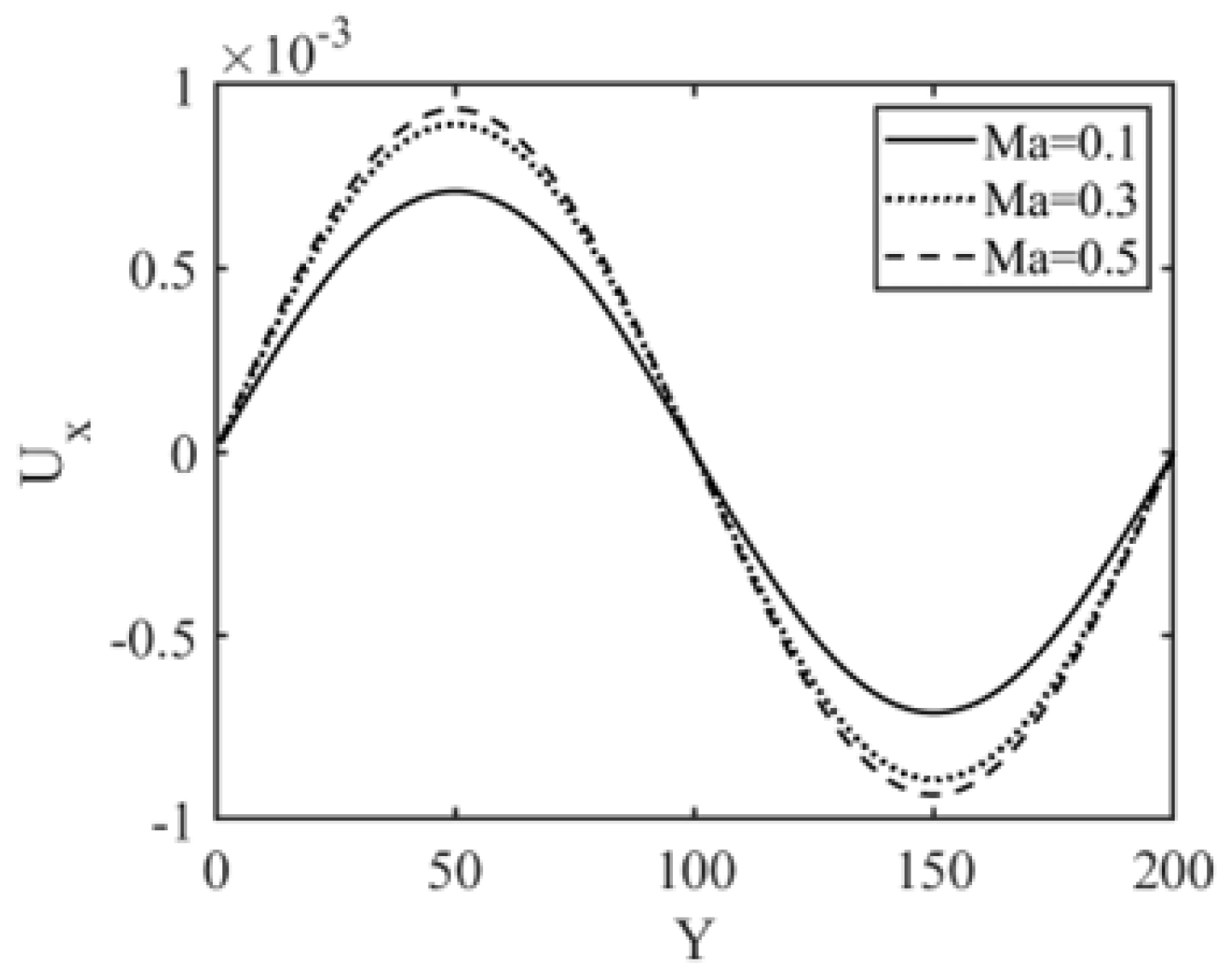
Firstly, the original model and the second-order direct projecting regularization reconstruction, as well as the third- and fourth-order recursive regularization reconstruction models, are used for tests when the temperature value is set to the lattice reference temperature. As the results of all the models are similar, only the results of the original model are presented here in Figure 1.

Figure 1.
ux distribution curves of the original model at different Mach numbers under the lattice reference temperature.
After ten convection periods at different Mach numbers, the attenuation degree of the x-direction velocity varies, but all correspond to the same numerical viscosity. This viscosity is a function of the maximum x-direction velocity and time, which can be obtained through formula fitting. Further comparisons between the original model and the second-order direct projecting regularization reconstruction, as well as the third- and fourth-order recursive regularization reconstruction models, are shown in Table 1. It can be seen that, although the second-order direct projecting regularization model can accurately calculate the numerical viscosity value when the Mach number is less than 0.5, its stability is significantly worse compared to the original model. The third- and fourth-order recursive regularization reconstruction models, like the original model, can accurately predict the numerical viscosity in this example even when the Mach number reaches up to 0.6. When the Mach number further increases to 0.7, the original model diverges, resulting in non-numerical results. Although the third- and fourth-order recursive regularization reconstruction models yield non-physical negative viscosity coefficient results, the calculations do not diverge. It can be seen that the regularization method still has the Galilean invariance characteristic, just like the original model. Moreover, in this example, it indicates that the direct projecting regularization method is not recommended due to stability issues, and at least the third-order recursive regularization model should be used.

Table 1.
Numerical viscosity calculated for different models at different Mach numbers under the lattice reference temperature.
Next, with the Mach number fixed at 0.1, we test the four models when the temperature deviates from the lattice reference temperature. The comparison between the original model and the second-order direct projecting regularization reconstruction, as well as the third-order and fourth-order recursive regularization reconstruction models, is presented in Table 2. It can be seen that both the original model and the regularization models can calculate the correct numerical viscosity over a wide temperature range. The original model and the second-order direct projecting regularization model exhibit similar stability ranges, while the stability ranges of the third-order and fourth-order recursive regularization reconstruction models are broader than those of the previous two models in the temperature range above the lattice reference temperature.
Table 2.
Numerical viscosity calculated for different models at different temperatures when the Mach number is 0.1.
3.2. Stability Tests
The stability of the proposed model is tested using the periodic double-shear layer flow. The initial conditions for the test are as follows:
where represents the length of the computational domain in both x and y directions, denotes the characteristic velocity, signifies the disturbance in velocity in the y direction, and controls the width of the shear layer. The Reynolds number is defined as . Temperature values vary depending on different cases. The lattice reference temperature is set to .
3.2.1. Flow at Lattice Reference Temperature
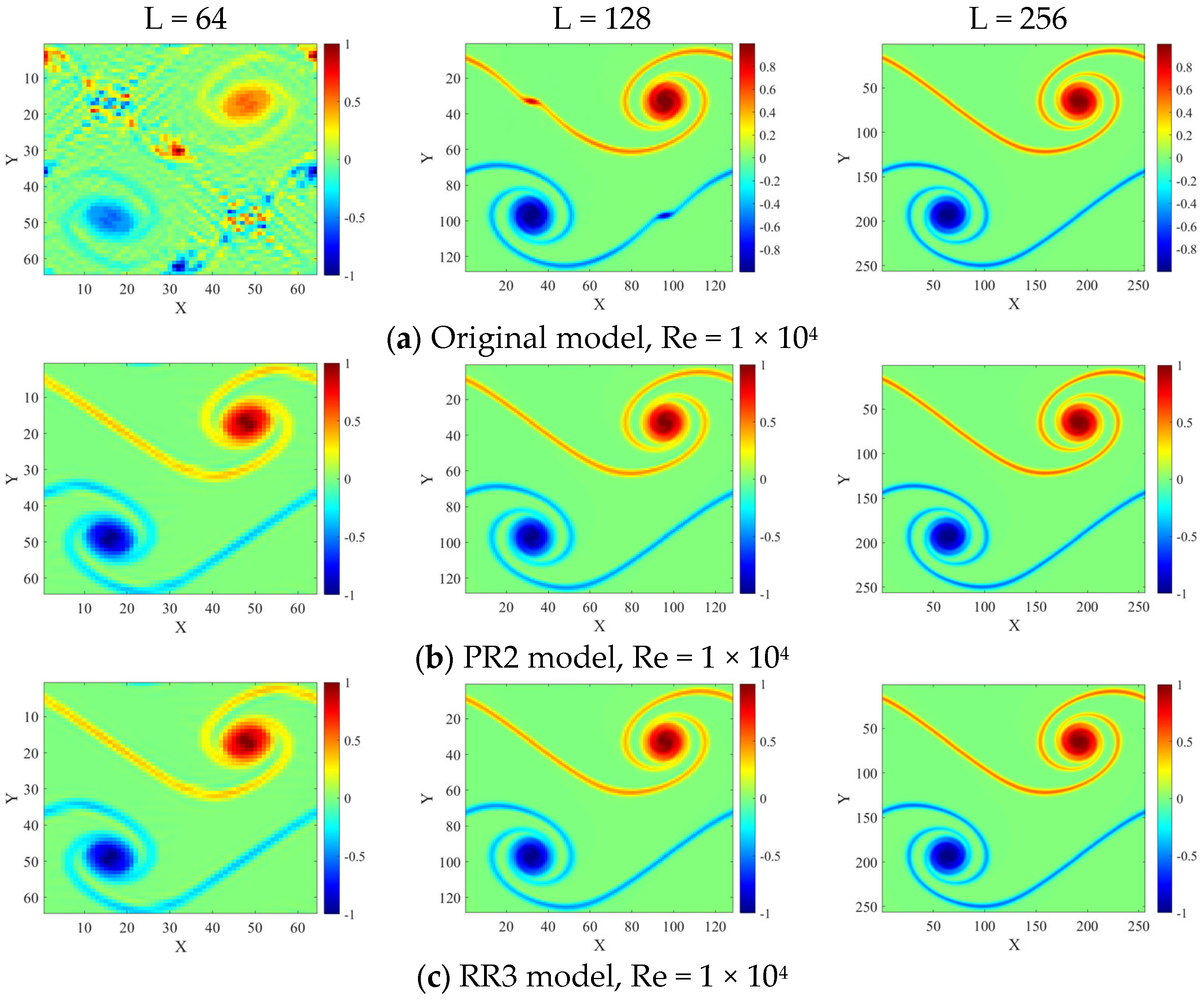
The temperature is set to . The stability ranges of the original model, the direct projecting regularization model, and the third-order recursive regularization model are studied. Initially, the three models are employed to simulate validation cases at varying grid resolutions (64 × 64, 128 × 128, and 256 × 256). The stability of the models is investigated by calculating double-shear layers at different Reynolds numbers and velocities. The calculation duration is one convective period, . The results are presented in Figure 2, with grid resolutions of 64 × 64, 128 × 128, and 256 × 256, from left to right. It can be observed from the results that when the Reynolds number is set to and the characteristic velocity is , the original model diverges at the 64 × 64 grid scale, and there are spurious vortices at the 128 × 128 grid scale, which further leads to computational instability. Satisfactory results can be obtained at the 256 × 256 grid scale. For both the direct projecting second-order regularization model and the third-order recursive regularization model, stable results can be obtained at different grid resolutions.
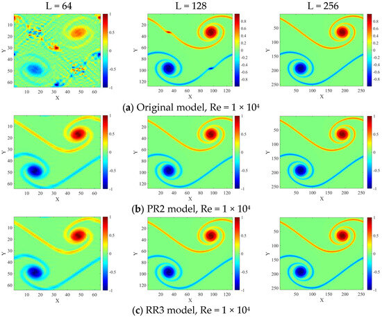
Figure 2.
Results of three models with the Reynolds number Re = 1 × 10⁴ and an initial velocity of 0.1 lattice units.
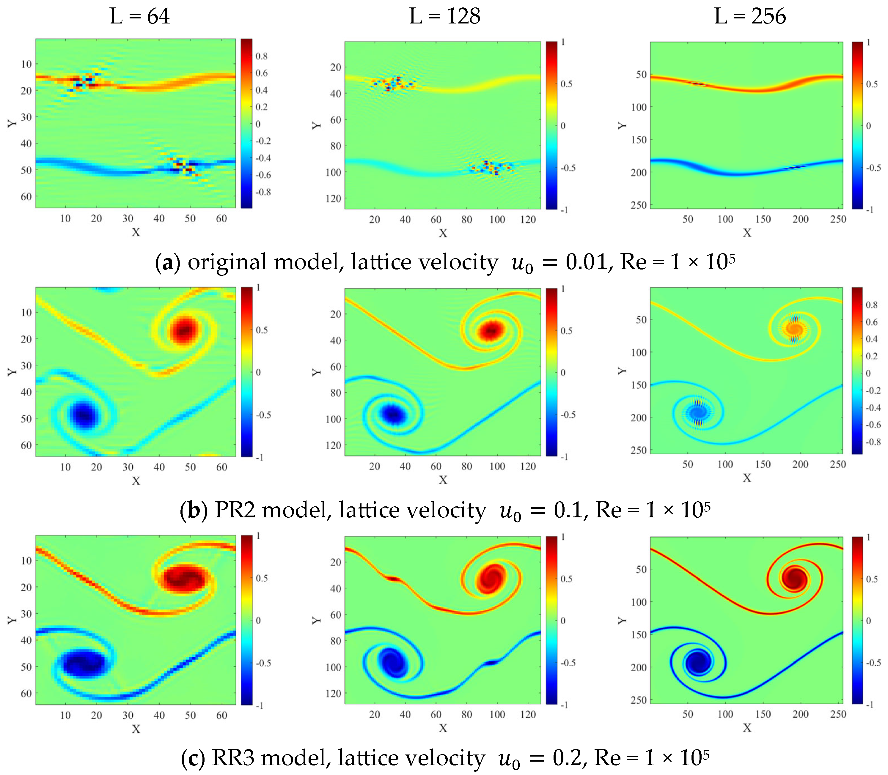
When the Reynolds number is set to , the results are shown in Figure 3, with grid resolutions from left to right being 64 × 64, 128 × 128, and 256 × 256. As can be seen from the figure, even when the characteristic velocity is , the original model quickly diverges at different grid scales. For the direct projecting second-order regularization model with characteristic velocity , there are spurious vortices in the results at grid scales of 64 × 64 and 128 × 128, which further leads to computational instability. Divergence occurs when using the refined grid scale of 256 × 256. For the third-order recursive regularization model with characteristic velocity , there are spurious vortices in the results at grid scales of 64 × 64 and 128 × 128. However, stable and accurate results can be obtained after using the refined grid scale of 256 × 256.
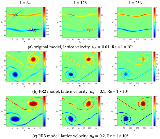
Figure 3.
Results of three models with the Reynolds number Re = 1 × 10⁵ and lattice reference temperature.
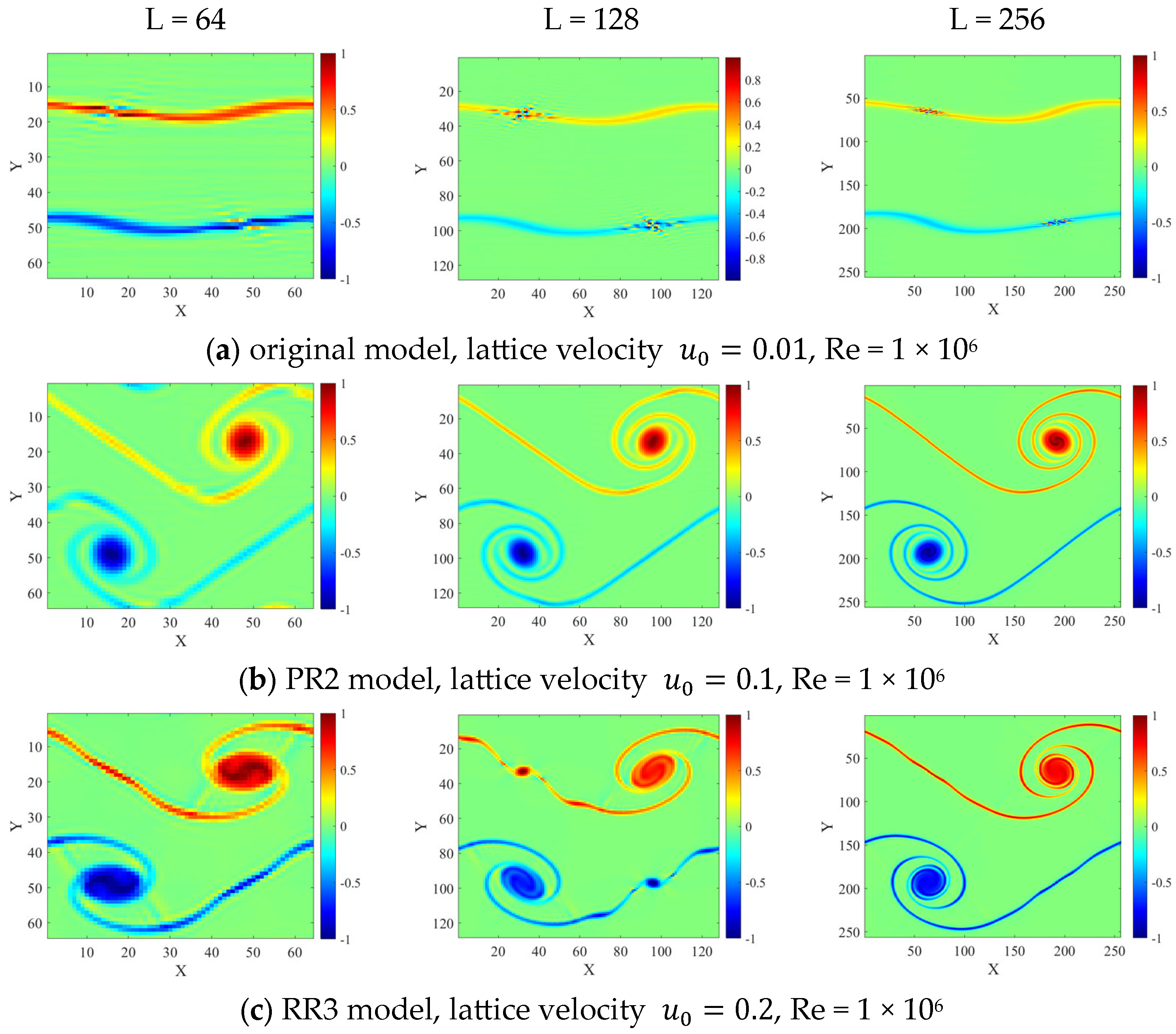
When the Reynolds number is set to Re = 1 × 10⁶, the results are shown in Figure 4. The grid resolutions from left to right are 64 × 64, 128 × 128, and 256 × 256, respectively. As can be seen from the results, at this Reynolds number, even when the characteristic velocity is set to 0.01 lattice units for the original model, stable calculations cannot be achieved at different grid scales. For the second-order direct projecting model, when the characteristic velocity is 0.05 lattice units, calculations can be performed stably, and satisfactory results can be obtained at the refined grid scale of 256 × 256. For the third-order recursive regularization model, even when the characteristic velocity is 0.2 lattice units, although there are spurious vortices at coarse grid scales, the calculations do not diverge. Moreover, as the grid is refined, stable and accurate results can be obtained.
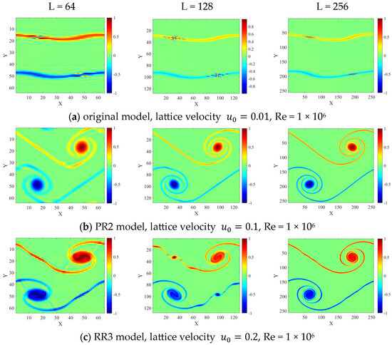
Figure 4.
Results of three models with the Reynolds number Re = 1 × 10⁶ and lattice reference temperature.
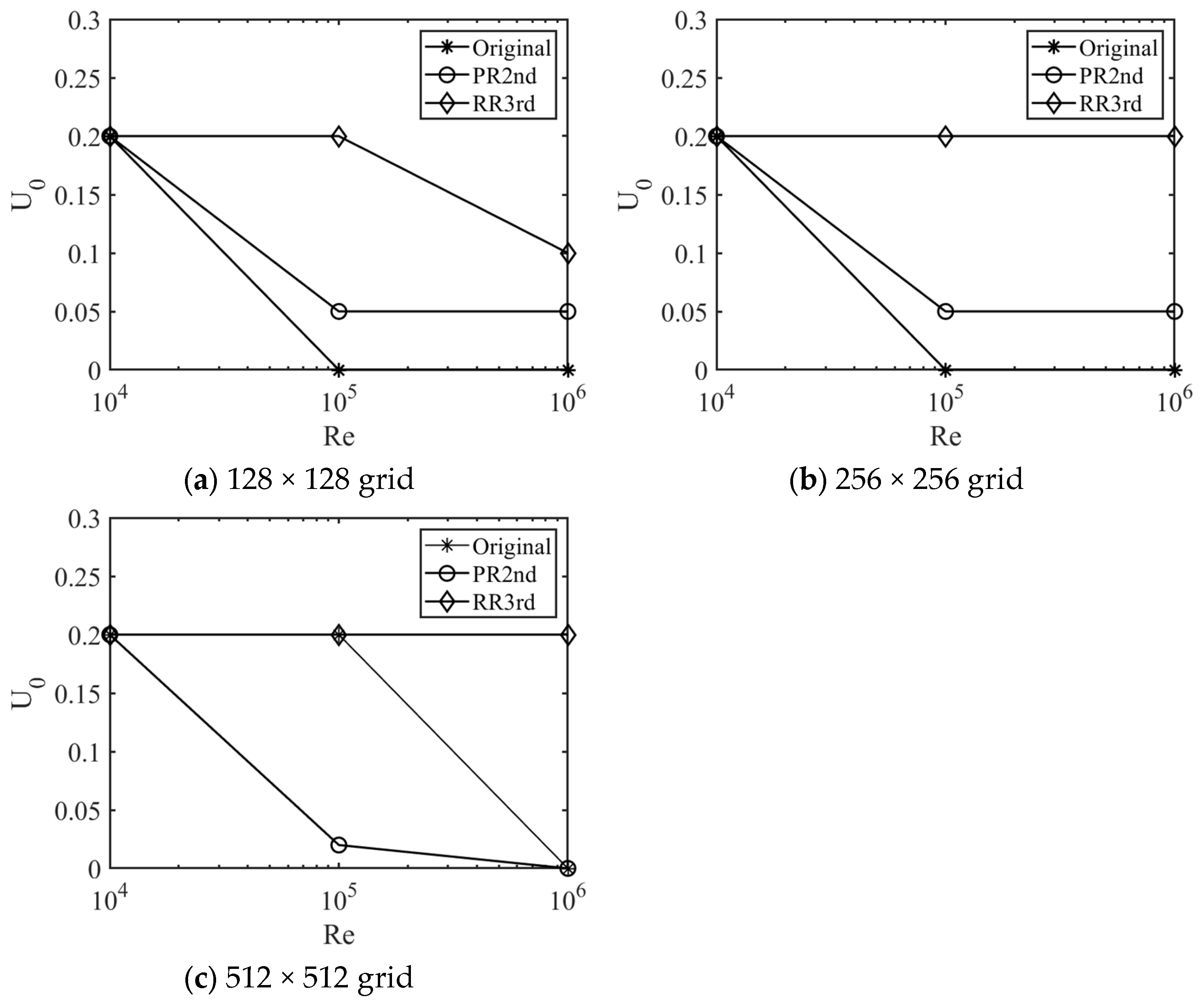
Next, we present the stability ranges of three models under different Reynolds numbers at various grid scales, specifically, the maximum velocity values that can be stably calculated at a fixed Reynolds number. During the testing process, if stable results cannot be obtained even when the minimum characteristic velocity (corresponding to a Mach number of approximately ) is taken, it is considered that the model cannot achieve stable results within this Reynolds number range. As can be seen from Figure 5, the third-order recursive regularization model exhibits excellent stability at different grid resolutions. For grid resolutions of both 256 × 256 and 512 × 512, stable calculations can be achieved at a higher characteristic velocity of (corresponding to a Mach number of approximately ) within the Reynolds number range from to . For the original model, stable results can only be obtained at a Reynolds number of when the grid resolution is 128 × 128 and 256 × 256, and the stable characteristic velocity can reach . When using a fine grid resolution of 512 × 512, stability is significantly improved, and stable calculation results can be obtained at , with the stable characteristic velocity reaching . For the second-order direct projecting model, when the grid resolution is 128 × 128 and 256 × 256, it exhibits almost the same stability, achieving stable calculation results at with the characteristic velocity reaching . However, at and , the characteristic velocity for achieving stable calculation results can only reach . It is worth noting that for the second-order direct projecting model, when the grid is further refined to a resolution of 512 × 512, its stability actually decreases. Correspondingly, the characteristic velocity at which stable results are obtained decreases from to when , while the model fails to obtain stable results when . This phenomenon of decreased stability in direct projecting schemes during grid refinement is similar to that observed by Christophe Coreixas et al. in their study of recursive regularization high-order expansions for the LBM-BGK method [29]. The specific mathematical and physical issues underlying this phenomenon require further exploration.

Figure 5.
Stability of three models at different grid resolutions.
3.2.2. Flow at Temperature Deviating from the Lattice Reference Temperature
From the research in the previous section, it can be observed that when the computational temperature is fixed at the lattice reference temperature , the third-order recursive regularization model significantly improves the computational stability compared to the original model and the second-order direct projecting regularization model. Furthermore, among the three LBM models, the second-order direct projecting regularization model can filter out non-hydrodynamic modes at lower grid resolutions but may exhibit stability issues when the grid is refined. Therefore, in the subsequent research, the second-order direct projecting regularization model will not be used, and the main focus will be on comparing the performance of the original model and the third- and fourth-order recursive regularization models when the computational temperature deviates from the lattice reference temperature.
The temperature range that can be used by the LBM solver for compressible thermal flows has a significant impact on its practical application in simulating engineering and scientific problems. For the study of some chemical reaction flow problems with significant temperature differences and heat absorption/release effects, it is particularly important for the solver to be able to operate over a wide temperature range. In addition to the temperature range, another consideration is the available Reynolds number range, as many engineering problems involve situations where the Reynolds number is relatively high. In this section, the characteristic flow velocity is set to in lattice units, which corresponds to a Mach number of approximately 0.3 in lattice units, balancing the considerations of model stability and computational efficiency. With a fixed characteristic velocity, the performance of the original model and the third- and fourth-order recursive regularization models is tested under different grid resolutions and Reynolds numbers.
For the original model, the vorticity distribution at a Reynolds number of is shown in Figure 6, with grid resolutions of 128 × 128, 256 × 256, and 512 × 512, from left to right. As can be seen from the figure, at the Reynolds number of , the stable temperature range at different grid scales is relatively wide, with . Even with a coarse grid resolution of 128 × 128, stable results can be obtained. It can be seen that within this Reynolds number range, the original model can be used to calculate some scientific and engineering problems with significant temperature differences.
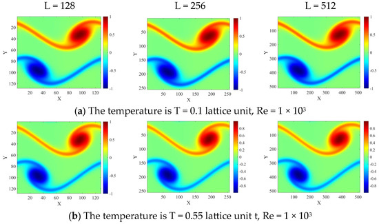
Figure 6.
Reynolds number Re = 1 × 10³, results of the original model at different temperatures.
The vorticity distribution when the Reynolds number increases to is shown in Figure 7. It can be seen from the figure that the stable temperature range is , and the stability region becomes significantly narrower. Moreover, when the temperature is set at 0.45, stability issues begin to emerge in computations with low-resolution grids, requiring grid refinement to obtain accurate results. Furthermore, when the Reynolds number increases to , stable results cannot be obtained within a narrow range deviating from the lattice reference temperature for computations at three different grid scales. Due to the narrow stable temperature range available in the original model at this Reynolds number, it loses the ability to simulate large temperature difference problems. Therefore, the vorticity distribution of the results at this Reynolds number is not presented here.
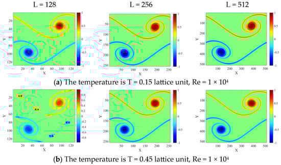
Figure 7.
Reynolds number Re = 1 × 10⁴, results of the original model at different temperatures.
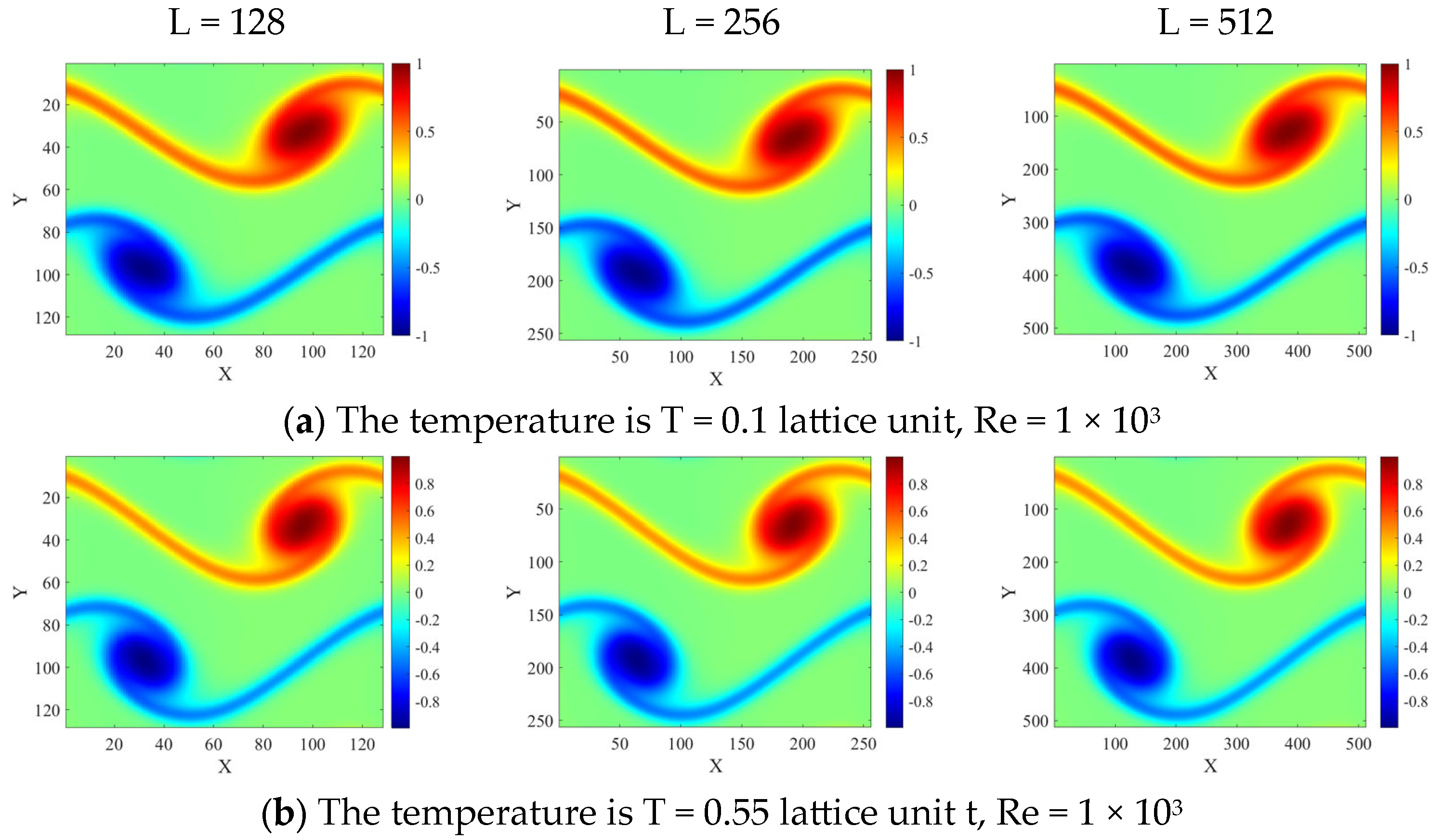
Next, we analyze the results of the third-order regularized model. The vorticity distributions are shown in Figure 8, Figure 9 and Figure 10, with grid resolutions of 128 × 128, 256 × 256, and 512 × 512 from left to right, respectively. As can be seen in Figure 8, when the Reynolds number is , the stable temperature range under different grid scales is relatively wide, with the temperature range ratio reaching , which is basically consistent with the stable range of the original model. As shown in Figure 9, when the Reynolds number increases to , the ratio of the stable temperature range is . Although the stability range slightly decreases with an increase in Reynolds number by an order of magnitude, the third-order regularized model still has a significant advantage compared to the original model’s stability range of .
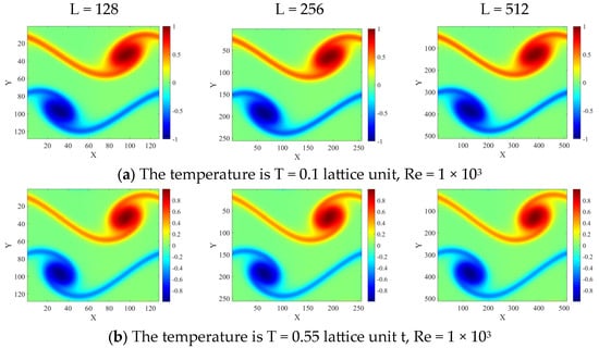
Figure 8.
Reynolds number Re = 1 × 10³, results of the RR3 model at different temperatures.
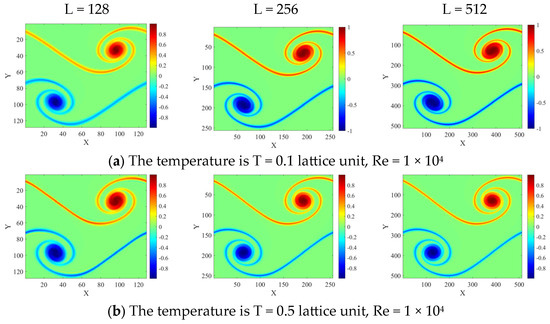
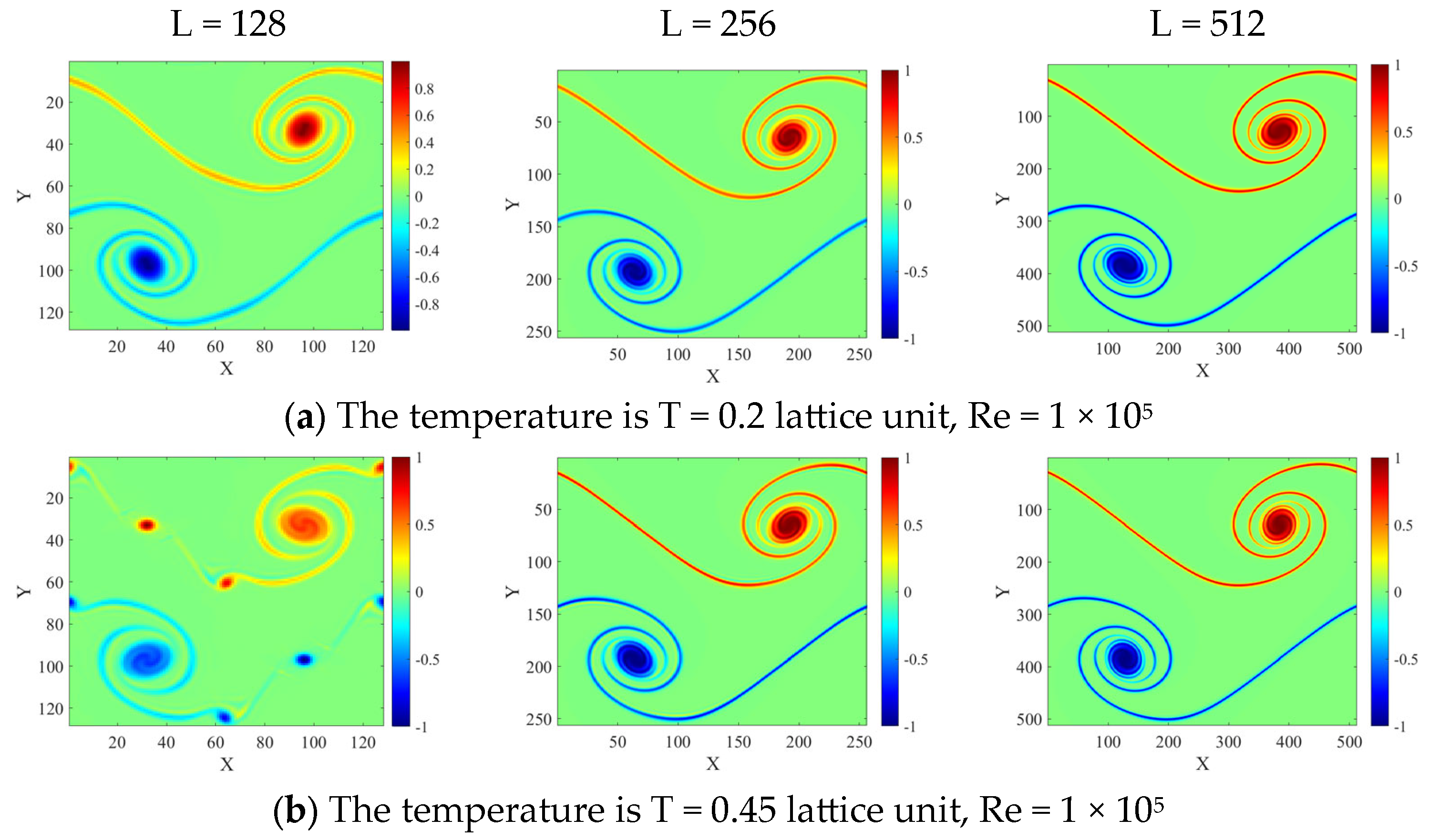
Figure 9.
Reynolds number Re = 1 × 10⁴, results of the RR3 model at different temperatures.
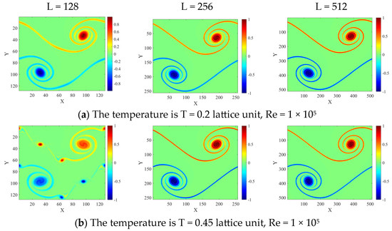
Figure 10.
Reynolds number Re = 1 × 10⁵, results of the RR3 model at different temperatures.
As the Reynolds number increases to , as shown in Figure 10, the stable temperature range is . At this Reynolds number, the stability region of the third-order regularized model significantly decreases. Moreover, when the temperature value is 0.45 and the grid resolution is 128 × 128, non-physical spurious vortices appear in the calculation, requiring grid refinement to obtain correct results. The appearance of spurious vortices at this low-resolution grid also indicates that the computational stability of the third-order regularized model begins to deteriorate under this configuration. Although the stability range of the third-order regularized model deteriorates at this Reynolds number, it still has significant advantages compared to the original model, which is basically unable to calculate stably under this condition.
To further expand the calculable temperature range of the thermally compressible LBM, the fourth-order recursive regularization model is employed for subsequent calculations. The results for Reynolds numbers Re = 1 × 10³ and Re = 1 × 10⁴ are presented in Figure 11 and Figure 12, respectively, with grid resolutions ranging from left to right as 128 × 128, 256 × 256, and 512 × 512. Evidently, in comparison to the original model and the third-order recursive regularization model, the fourth-order recursive regularization model significantly broadens the applicable temperature and velocity ranges of the thermally compressible LBM. As shown in Figure 11 for the case of Re = 1 × 10³, it can be observed that the stable temperature range ratio of the fourth-order regularization model can reach at all three grid resolutions, which is consistent with the stable calculation range of the original model.
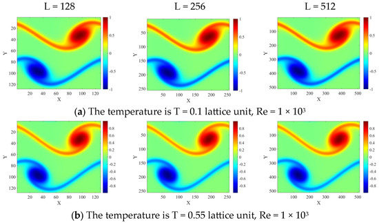
Figure 11.
Reynolds number Re = 1 × 10³, results of the RR4 model at different temperatures.
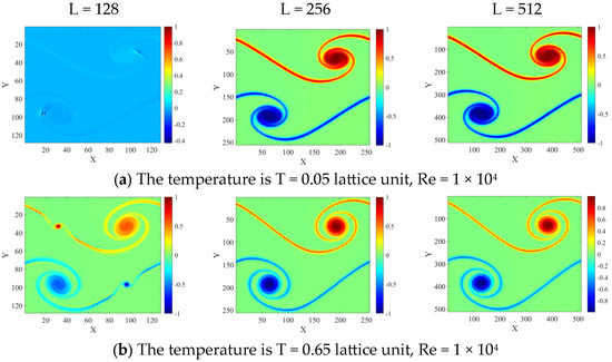
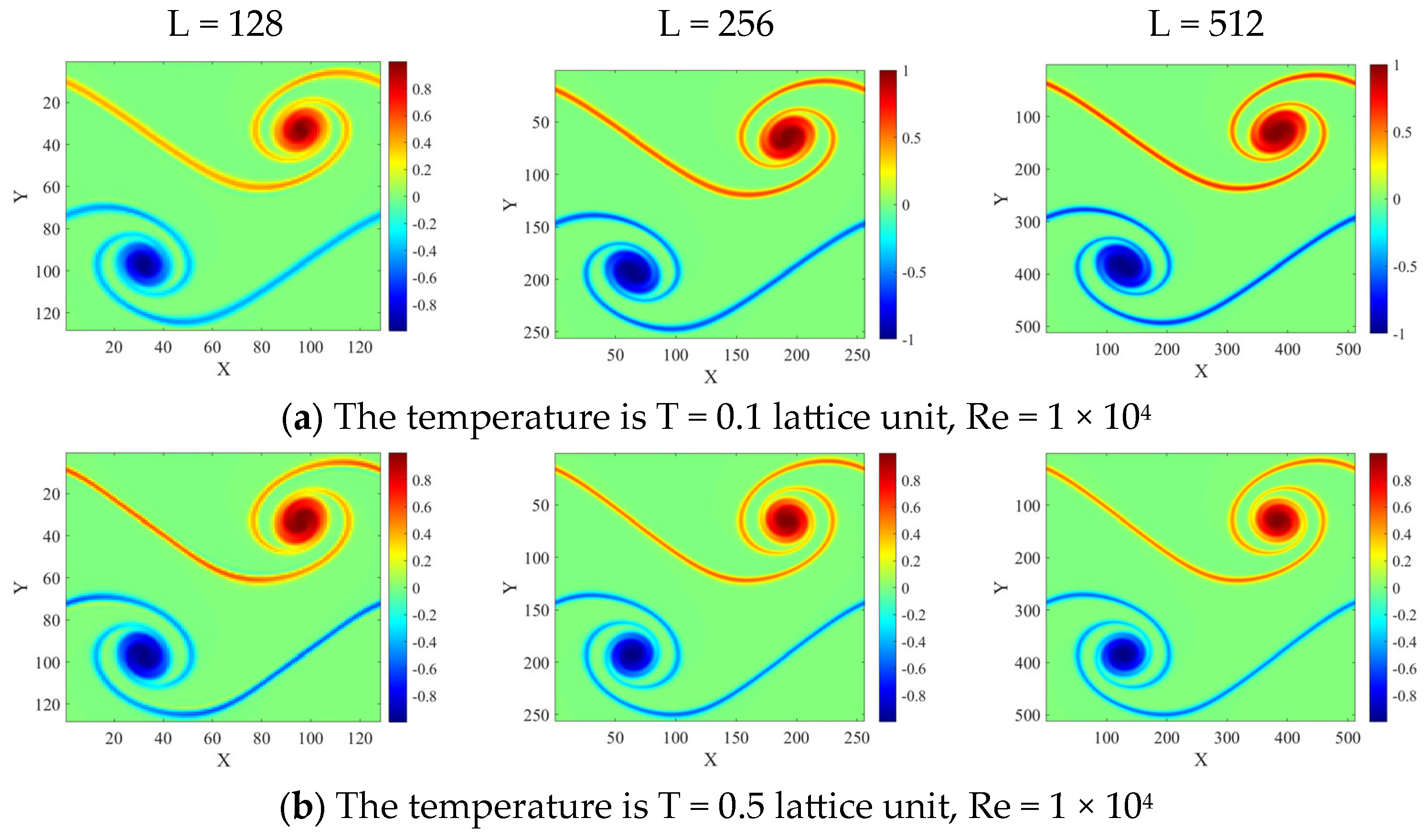
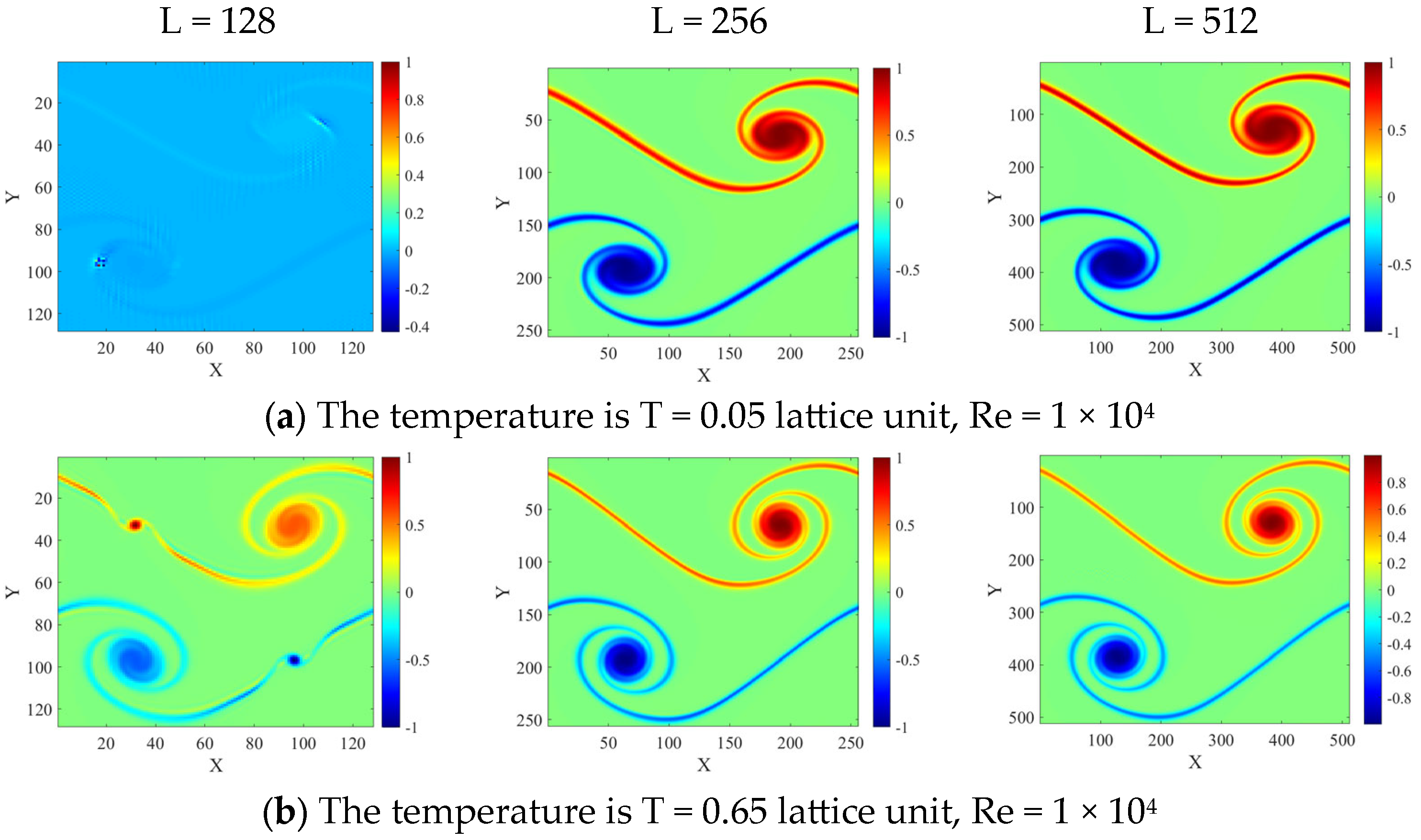
Figure 12.
Reynolds number Re = 1 × 10⁴, results of the RR4 model at different temperatures.
The results when the Reynolds number is set to Re = 1 × 10⁴ are shown in Figure 12. As can be seen from the figure, for the fourth-order regularized model, although the calculation diverges when using a coarse grid of 128 × 128 at a temperature of T = 0.05 lattice units, stable results can still be obtained with grid refinement. When the temperature is T = 0.65 lattice units, although there are two spurious vortices when using a coarse grid of 128 × 128, accurate results can be obtained when the grid is refined to 256 × 256.
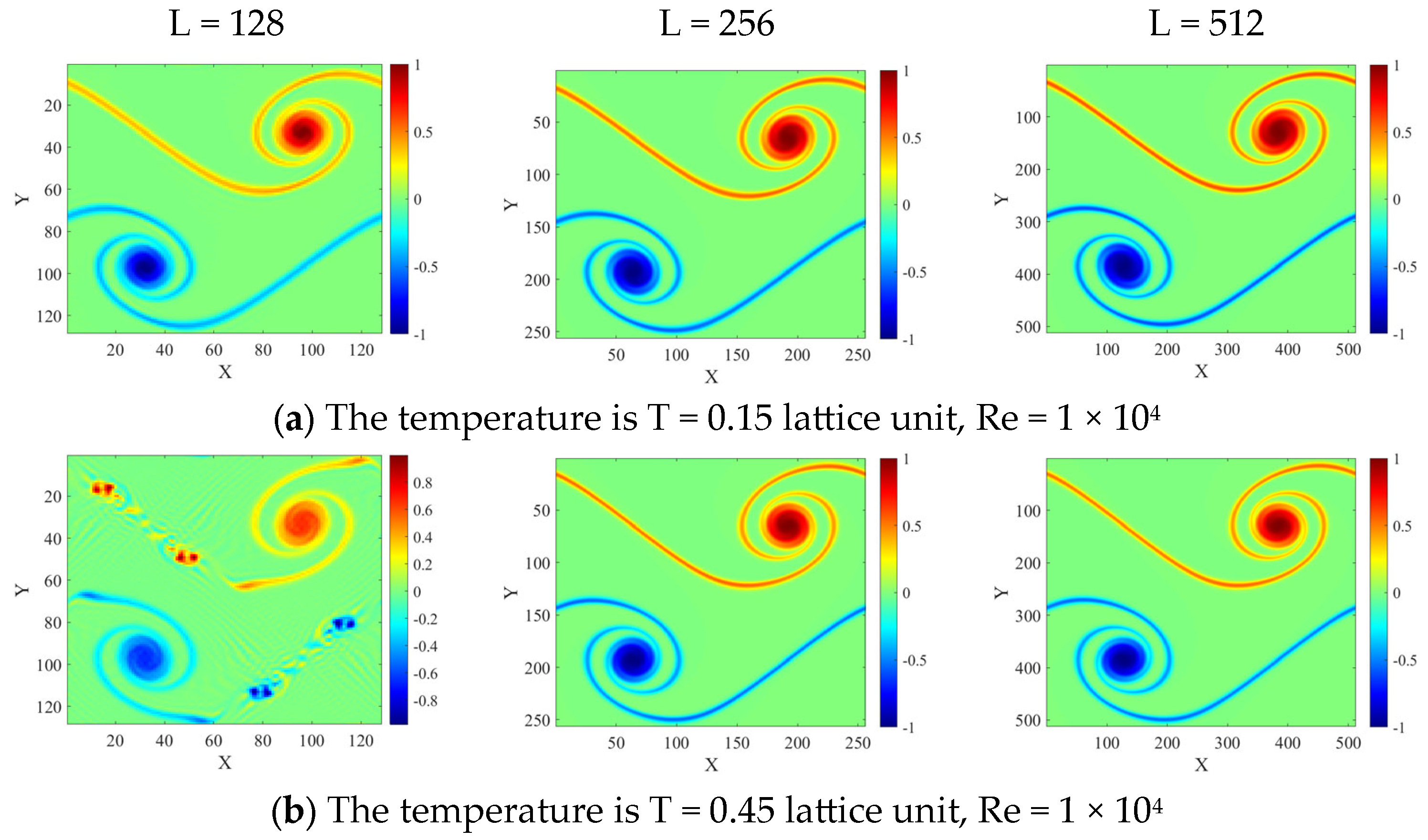
The results for a Reynolds number of Re = 1 × 10⁵ are shown in Figure 13, with grid resolutions of 128 × 128, 256 × 256, and 512 × 512, from left to right. A noteworthy observation is that when the Reynolds number is set to Re = 1 × 10⁵ and the lattice temperature is set to 0.15 lattice units, satisfactory results are achieved with grid refinement up to 256 × 256. However, further refinement to 512 × 512 leads to computational instability. This requires further investigation to elucidate the mathematical mechanism behind its occurrence. In the case of a Reynolds number of Re = 1 × 10⁵, compared to the third-order recursive regularization model, which can use a maximum temperature of 0.45 lattice units, the fourth-order recursive regularization model eliminates spurious vortices and achieves accurate results with grid refinement at a temperature of 0.55 lattice units.
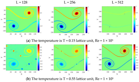
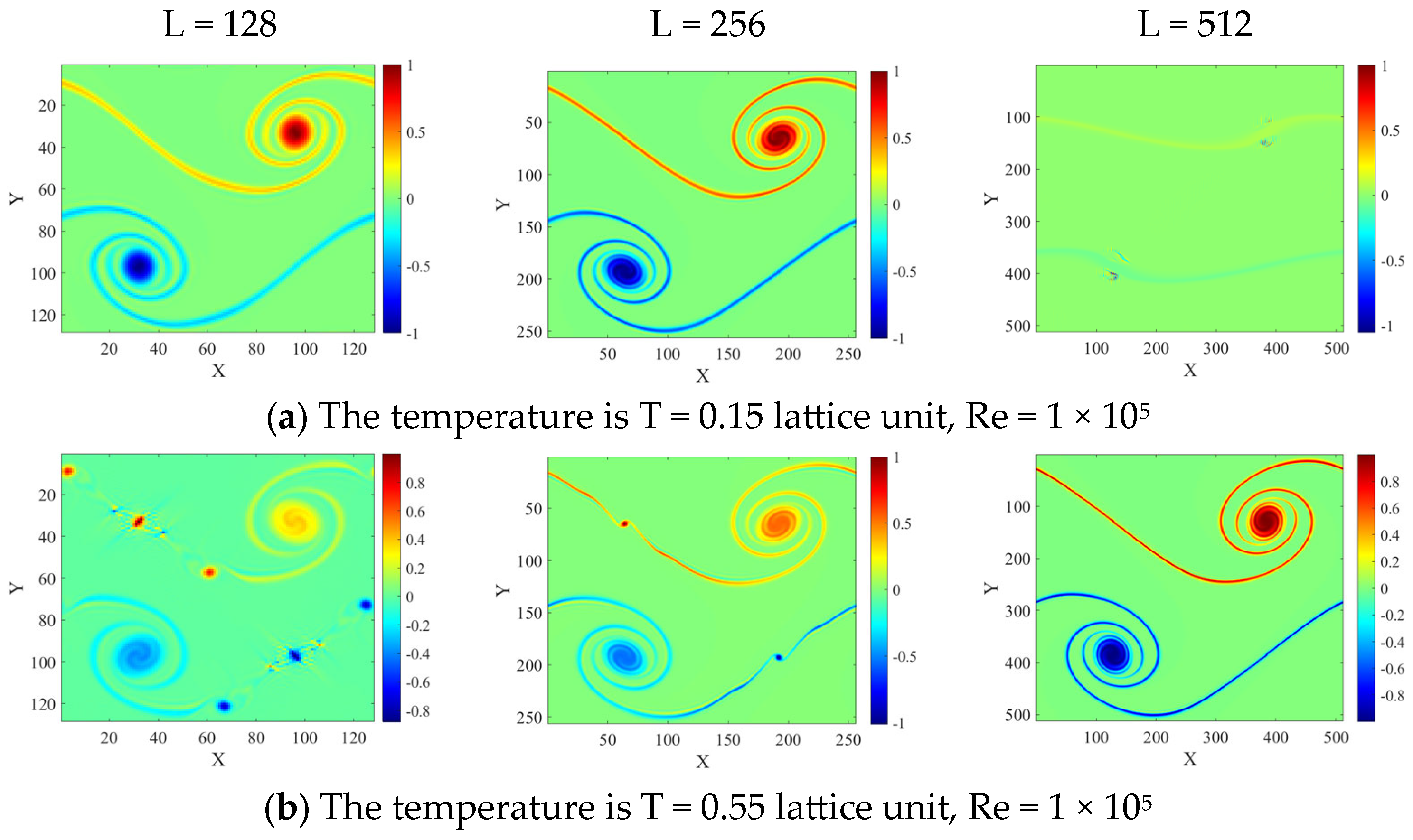
Figure 13.
Reynolds number Re = 1 × 10⁵, results of the RR4 model at different temperatures.
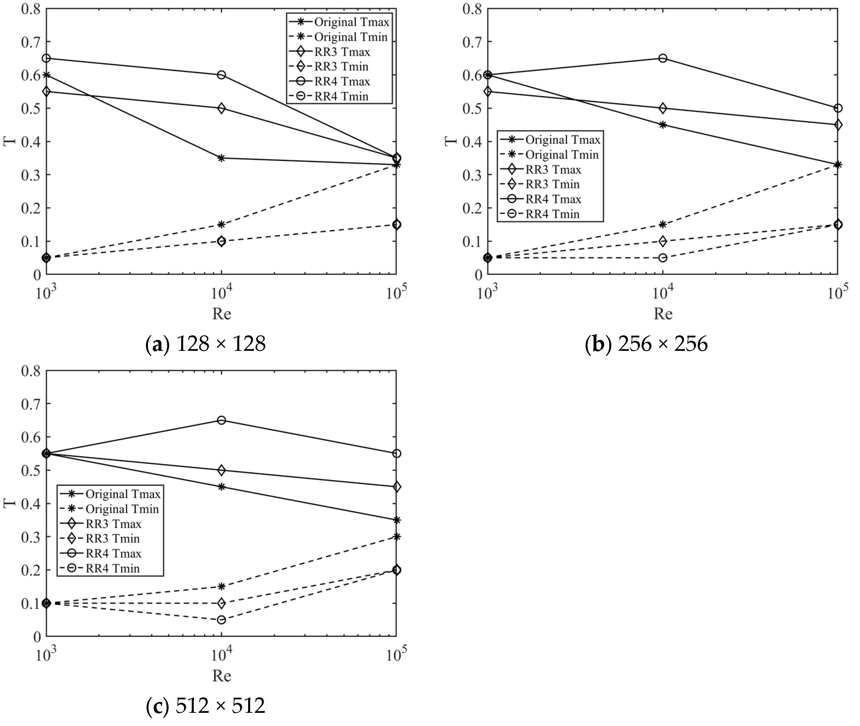
The comparison of the stable temperature range for the original model, third-order recursive regularization model, and fourth-order recursive regularization model under different grid resolutions and Reynolds numbers is shown in Figure 14. It can be observed that, overall, the stability of the third-order recursive regularization model is significantly improved compared to the original model, with the ability to calculate a wider temperature range under most grid parameters and Reynolds numbers. For the original model, the extent to which the stable calculation temperature range is widened by mesh refinement is limited, making it difficult to simulate examples with large temperature differences at high Reynolds numbers. The third-order recursive regularization model faces the same problem, and the mesh refinement does not significantly broaden the available temperature range. When the Reynolds number is , the stable temperature range is also significantly narrowed, which is not conducive to simulating thermal flow problems at high Reynolds numbers. In contrast, the fourth-order recursive regularization model is the most stable model within various parameter ranges. Moreover, when the Reynolds number is , its stable temperature range is significantly widened compared to the original model and the third-order recursive regularization model with mesh refinement. This allows for the possibility of using a thermally compressible LBM solver to simulate chemical reaction phenomena with severe heat release.
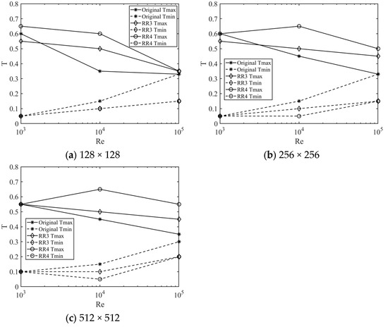
Figure 14.
The stable temperature range for three models at different grid resolutions under varying Reynolds numbers.
4. Conclusions
In this paper, a regularized reconstruction scheme is conducted for an extended equilibrium distribution thermal compressible LBM with corrected deviation terms. Direct projecting and recursive regularization methods are employed to reconstruct the non-equilibrium distribution function. The results indicate that the LBM model obtained through second-order regularized reconstruction using direct projecting significantly improves computational stability at lower grid resolutions. However, as the grid is refined, instability may occur. This phenomenon could be linked to the numerical instability that arises in high-velocity or high-Reynolds number simulations, which is a known challenge in lattice Boltzmann solvers due to the accumulation of higher-order non-hydrodynamic modes at finer grid resolutions. The underlying reasons for this phenomenon require further investigation. Both third- and fourth-order recursive regularization methods can significantly enhance the numerical stability of the model at different grid resolutions, broadening the application range in terms of speed and temperature compared with the original model. Notably, simulations of periodic double-shear flows demonstrate that the usable temperature range of the fourth-order recursive regularization model is significantly expanded when using higher velocities, which is meaningful for expanding the application scope of the LBM.
In addition, standard models such as D2Q9 or D3Q27 cannot describe the heat flux, so they need to be coupled with another distribution function, a traditional method such as finite volume, or finite difference methods for solving the energy equation. The focus of this work is to study the stability of the standard LBM when it deviates from the lattice reference temperature. In future work, the lattice Boltzmann solver developed in this work will be coupled with the finite difference method to simulate the thermal flow problems.
Author Contributions
Conceptualization, Z.Z.; Funding acquisition, H.G.; Methodology, Z.Z.; Project administration, H.G.; Software, Z.Z.; Validation, Z.Z. and Y.L.; Writing—original draft, Z.Z.; Writing—review and editing, Y.L. and H.G. All authors have read and agreed to the published version of the manuscript.
Funding
This research was funded by the National Key R&D Program of China (Grant No. 2021YFA0719200) Research Program.
Data Availability Statement
The data that support the findings of this study are available within the article.
Conflicts of Interest
The authors declare no conflicts of interest.
Abbreviations
The following abbreviations are used in this manuscript:
| LBM | Lattice Boltzmann method |
| CFD | Computational fluid dynamics |
| BGK | Bhatnagar–Gross–Krook |
References
- Dorschner, B.; Bösch, F.; Chikatamarla, S.S.; Boulouchos, K.; Karlin, I.V. Entropic multi-relaxation time lattice Boltzmann model for complex flows. J. Fluid Mech. 2016, 801, 623–651. [Google Scholar] [CrossRef]
- Wagner, A.J. Thermodynamic consistency of liquid-gas lattice Boltzmann simulations. Phys. Rev. E 2006, 74, 056703. [Google Scholar] [CrossRef]
- Tölke, J.; De Prisco, G.; Mu, Y. A lattice Boltzmann method for immiscible two-phase Stokes flow with a local collision operator. Comput. Math. Appl. 2013, 65, 864–881. [Google Scholar] [CrossRef]
- Montessori, A.; Prestininzi, P.; La Rocca, M.; Falcucci, G.; Succi, S.; Kaxiras, E. Effects of Knudsen diffusivity on the effective reactivity of nanoporous catalyst media. J. Comput. Sci. 2016, 17, 377–383. [Google Scholar] [CrossRef]
- Sawant, N.; Dorschner, B.; Karlin, I.V. Consistent lattice Boltzmann model for reactive mixtures. J. Fluid Mech. 2022, 941, A62. [Google Scholar] [CrossRef]
- Bocanegra Cifuentes, J.A.; Borelli, D.; Cammi, A.; Lomonaco, G.; Misale, M. Lattice Boltzmann Method Applied to Nuclear Reactors—A Systematic Literature Review. Sustainability 2020, 12, 7835. [Google Scholar] [CrossRef]
- Bocanegra, J.A.; Misale, M.; Borelli, D. A systematic literature review on Lattice Boltzmann Method applied to acoustics. Eng. Anal. Bound. Elem. 2024, 158, 405–429. [Google Scholar] [CrossRef]
- Sharma, K.V.; Straka, R.; Tavares, F.W. Current status of Lattice Boltzmann Methods applied to aerodynamic, aeroacoustic, and thermal flows. Prog. Aerosp. Sci. 2020, 115, 100616. [Google Scholar] [CrossRef]
- Perumal, D.A.; Dass, A.K. A Review on the development of lattice Boltzmann computation of macro fluid flows and heat transfer. Alex. Eng. J. 2015, 54, 955–971. [Google Scholar] [CrossRef]
- Succi, S. The Lattice Boltzmann Equation: For Complex States of Flowing Matter; Oxford University Press: Oxford, UK, 2018. [Google Scholar]
- Krüger, T.; Kusumaatmaja, H.; Kuzmin, A.; Shardt, O.; Silva, G.; Viggen, E.M. The Lattice Boltzmann Method: Principles and Practice; Springer: Cham, Switzerland, 2017; Volume 10, pp. 4–15. [Google Scholar]
- Saadat, M.H.; Hosseini, S.A.; Dorschner, B.; Karlin, I.V. Extended lattice Boltzmann model for gas dynamics. Phys. Fluids 2021, 33, 046104. [Google Scholar] [CrossRef]
- Shan, X.; Yuan, X.F.; Chen, H. Kinetic theory representation of hydrodynamics: A way beyond the Navier–Stokes equation. J. Fluid Mech. 2006, 550, 413–441. [Google Scholar] [CrossRef]
- Chikatamarla, S.S.; Karlin, I.V. Lattices for the lattice Boltzmann method. Phys. Rev. E 2009, 79, 046701. [Google Scholar] [CrossRef]
- Li, X.; Shi, Y.; Shan, X. Temperature-scaled collision process for the high-order lattice Boltzmann model. Phys. Rev. E 2019, 100, 013301. [Google Scholar] [CrossRef]
- Frapolli, N.; Chikatamarla, S.S.; Karlin, I.V. Entropic lattice Boltzmann model for gas dynamics: Theory, boundary conditions, and implementation. Phys. Rev. E 2016, 93, 063302. [Google Scholar] [CrossRef]
- Wilde, D.; Krämer, A.; Reith, D.; Foysi, H. Semi-Lagrangian lattice Boltzmann method for compressible flows. Phys. Rev. E 2020, 101, 053306. [Google Scholar] [CrossRef]
- Prasianakis, N.I.; Karlin, I.V. Lattice Boltzmann method for simulation of compressible flows on standard lattices. Phys. Rev. E 2008, 78, 016704. [Google Scholar] [CrossRef]
- Prasianakis, N.I.; Karlin, I.V.; Mantzaras, J.; Boulouchos, K.B. Lattice Boltzmann method with restored Galilean invariance. Phys. Rev. E 2009, 79, 066702. [Google Scholar] [CrossRef]
- Guo, Z.; Zheng, C.; Shi, B.; Zhao, T.S. Thermal lattice Boltzmann equation for low Mach number flows: Decoupling model. Phys. Rev. E 2007, 75, 036704. [Google Scholar] [CrossRef]
- Feng, Y.; Sagaut, P.; Tao, W. A three dimensional lattice model for thermal compressible flow on standard lattices. J. Comput. Phys. 2015, 303, 514–529. [Google Scholar] [CrossRef]
- Saadat, M.H.; Bösch, F.; Karlin, I.V. Lattice Boltzmann model for compressible flows on standard lattices: Variable Prandtl number and adiabatic exponent. Phys. Rev. E 2019, 99, 013306. [Google Scholar] [CrossRef]
- Hosseini, S.A.; Darabiha, N.; Thévenin, D. Compressibility in lattice Boltzmann on standard stencils: Effects of deviation from reference temperature. Philos. Trans. R. Soc. A 2020, 378, 20190399. [Google Scholar] [CrossRef]
- Lallemand, P.; Luo, L.S. Theory of the lattice Boltzmann method: Acoustic and thermal properties in two and three dimensions. Phys. Rev. E 2003, 68, 036706. [Google Scholar] [CrossRef]
- Wissocq, G.; Sagaut, P.; Boussuge, J.F. An extended spectral analysis of the lattice Boltzmann method: Modal interactions and stability issues. J. Comput. Phys. 2019, 380, 311–333. [Google Scholar] [CrossRef]
- D’Humieres, D. Generalized Lattice-Boltzmann Equations. Rarefied Gas Dyn. Theory Simul. 1992, 159, 450–458. [Google Scholar]
- Wissocq, G.; Coreixas, C.; Boussuge, J.F. Linear stability and isotropy properties of athermal regularized lattice Boltzmann methods. Phys. Rev. E 2020, 102, 053305. [Google Scholar] [CrossRef]
- Latt, J.; Chopard, B. Lattice Boltzmann method with regularized pre-collision distribution functions. Math. Comput. Simul. 2006, 72, 165–168. [Google Scholar] [CrossRef]
- Coreixas, C.; Wissocq, G.; Puigt, G.; Boussuge, J.F.; Sagaut, P. Recursive regularization step for high-order lattice Boltzmann methods. Phys. Rev. E 2017, 96, 033306. [Google Scholar] [CrossRef]
- Jacob, J.; Malaspinas, O.; Sagaut, P. A new hybrid recursive regularised Bhatnagar–Gross–Krook collision model for lattice Boltzmann method-based large eddy simulation. J. Turbul. 2018, 19, 1051–1076. [Google Scholar] [CrossRef]
- Saadat, M.H.; Dorschner, B.; Karlin, I. Extended lattice Boltzmann model. Entropy 2021, 23, 475. [Google Scholar] [CrossRef]


Disclaimer/Publisher’s Note: The statements, opinions and data contained in all publications are solely those of the individual author(s) and contributor(s) and not of MDPI and/or the editor(s). MDPI and/or the editor(s) disclaim responsibility for any injury to people or property resulting from any ideas, methods, instructions or products referred to in the content. |
© 2025 by the authors. Licensee MDPI, Basel, Switzerland. This article is an open access article distributed under the terms and conditions of the Creative Commons Attribution (CC BY) license (https://creativecommons.org/licenses/by/4.0/).