Abstract
We introduce the solver ARES: Axial-flow pump Radial Equilibrium through Streamlines. The code implements a meanline method, enforcing the conservation of flow momentum and continuity across a set of discrete streamlines in the axial-flow pump’s meridional channel. Real flow effects are modeled with empirical correlations, including off-design deviation and losses due to profile shape, secondary flows, tip leakage, and the end-wall boundary layer (EWBL). Inspired by aeronautical fan and compressor methods, this implementation is specifically tailored for the analysis of the Outboard Dynamic-inlet Waterjet (ODW), the latest aero-engine-derived innovation in marine engineering. To ensure the reliable application of ARES for the systematic designs of ODW pumps, the present investigation focuses on prediction accuracy. Global and local statistics are compared between numerical estimates and available measurements of three test cases: two single rotors and a rotor–stator waterjet configuration. At mass flow rates near the design point, hydraulic efficiency is predicted within discrepancy to tests. Differently, as the flow coefficient increases, the loss prediction accuracy degrades, incrementing the error for off-design estimates. Spanwise velocity and pressure distributions exhibit good alignment with experiments near midspan, especially at the rotor exit, while end-wall boundary layer complex dynamics are hardly recovered by the present implementation.
1. Introduction
Outboard Dynamic-inlet Waterjets (ODW) have recently emerged as a real alternative in marine propulsion [1]. Advanced by industrial technology, this machine consists of an axisymmetric hydrodynamic nacelle shrouding a propulsive axial- or mixed-flow pump [2]. Submerged operation offers several advantages over existing solutions, including a uniform mass flow rate to the pump, no hull disturbance, no flow obstruction by the shaft, and alignment among the capture stream, thrust, and direction of advance—all addressing known limitations in naval propulsion [3,4,5,6,7,8].
To efficiently exploit the benefits of this configuration, the machinery requires a dedicated design. To this end, Blade Elements Methods (BEMs) have traditionally proved valuable techniques, enabling fast though accurate preliminary predictions of machines’ fluid dynamics [9]. Their advantage relies on the possibility of solving simplified flow equations while iterating through to introduce real flow effects as empirical external correlations. These models can be both experimental and numerical, with the work from Lieblein [10] setting the milestone reference in this field. In that study, planar blade cascade systematic measurements have served as the definition of several losses and deviation correlations against the incidence angle. Henceforth, the majority of the meanline methods for both compressible and incompressible applications has relied on those models [11,12,13,14,15,16,17], and many other theories have been developed over the years [18,19,20,21,22]. Although the estimates of BEM codes may reach significant accuracy levels, verification with high-fidelity Computational Fluid Dynamics (CFD) [23,24] and validation through experiments [25,26,27] are still mandatory steps.
To address the lack of existing methods for comprehensive ODW design, this study introduces ARES (Axial-flow pump Radial Equilibrium through Streamlines), a novel meanline solver specifically developed to predict ODW propulsive performance by modeling the interaction between the nacelle and the machine. The study focuses on the accuracy of the pump design module, which implements a BEM by enforcing flow momentum and continuity conservation and integrating these laws across streamlines. These axisymmetric surfaces discretize the machine’s meridional section spanwise and are designed as Blade Elements (BEs) using the 2D planar cascades assumption. This approach leverages well-established correlations to model in- and off-design deviations, losses, and other real flow effects. Three axial-flow pump test cases from the literature are selected to compare global and local measurements with the ARES solution.
2. Methods
The present method solves the axial-flow pump meanline flow, relying on the satisfaction of continuity and momentum conservation laws, with the latter often labeled as the Radial Equilibrium (RE) equation. The differential laws integrals are computed across a finite number of BEs or streamlines adopted to discretize the machine meridional plane. The iterative routine marches while updating the primary variables, introducing empirical and numerical correlations to model specific flow effects. Under these hypotheses, the present implementation is effectively a lumped-element model, where flow conditions are evaluated at specific radial locations along streamwise stations. The empirical correlations are leveraged to model real-world fluid phenomena without solving their evolution. Specifically, the model assumes the geometry designed from 2D planar cascades allows for the adoption of several well-established approaches capable of modeling the primary 2D and 3D axial-flow machinery flow effects. Finally, consistency across the entire channel is ensured by iterating through the fluid dynamics fundamental laws. The complete implementation was independently carried out in Python 3.12.
2.1. Assumptions
The assumptions adopted to solve the governing equations are listed below:
- The flow is incompressible, where ;
- The flow is stationary, i.e., ;
- The solution holds at planes perpendicular to the axis, which are placed downstream of each blade row (red stations in Figure 1);
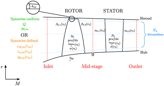 Figure 1. Schematic of a pump stage meridional view, including the domain discretization, input variables, and parameters required by the solver.
 - At each plane, the RE is integrated through streamlines, or BE (Figure 1), which are conceived as independent, axisymmetric surfaces of revolution about the machine axis. The corresponding spanwise location is iterated through to impose a mass flow balance, rather than employing constant radial increments, to enforce continuity within streamtubes;
- The flow is inviscid: viscous effects are modelled using empirical correlations and introduced upon the equation’s solution.
The streamtube flow is regulated by cascade shapes stacked to generate the blade’s entire span. Thus, hub-to-shroud distributions of the key geometrical parameters are required as input, as reported in Figure 1.
Figure 2 illustrates a schematic of the blade cascade quantities.
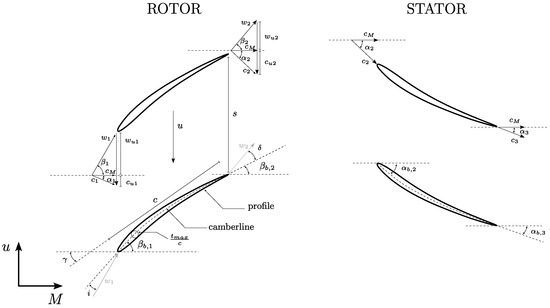
Figure 2.
Blade geometrical and flow quantities for a sample axial-flow pump stage section.
The absolute and relative velocities are denoted by c and w, respectively. The absolute and relative flow angles are represented by and , with a subscript b used to distinguish them from blade metal angles. The differences between flow-related and geometrical parameters define the leading edge incidence (i) and trailing edge deviation () angles.
Blade cascade flow behavior is characterized by velocity diagrams, showing velocity components in the meridional (M) and tangential (u) directions aligned with the machine axis and blade row speed, respectively. Key parameters include the profile maximum thickness (), normalized by the chord length (c); stagger angle (), calculated as the average between inlet and outlet metal angles; profile camber (); tip clearance (); and blade solidity (), the ratio of chord to blade pitch. Blade pitch (s) is determined by the radial location and number of blades () as .
A summary of the relevant blade cascades quantities adopted for ARES modeling is reported in Table 1.

Table 1.
Summary of relevant blade cascades parameters.
2.2. Governing Equations
According to Serovy et al. [12], momentum conservation is expressed as follows:
where g is the gravitational acceleration, h is the static head, and derivatives are computed along the radial, r, and axial, M, directions. Upon introducing the definition of the total head, , Equation (3) is then integrated between streamlines j and . Neglecting the variation in the radial component, , and including the definitions of both the energy exchange and the velocity diagram across a blade row, the finite difference solution of the problem may be formulated as follows:
where the coefficients are defined below, depending on flow quantities at an axial station and on the head losses, :
Equation (4) yields the meridional velocity at a certain streamline . Thus, starting from a given condition at , the spanwise distribution of at a given axial station i can be computed. Starting from the inflow boundary conditions, the solution marches downstream row by row. Iterations are necessary, since the radial locations of the streamlines are recursively revised and so are the corresponding flow quantities.
Finally, to impose continuity, the axial velocity profile is verified to satisfy mass conservation. Here, the volume flow rate is computed using the quadrature:
2.3. Implementation
ARES takes a formatted parameter file as input, which must contain fluid properties, complete hub-to-shroud geometrical characterization of the blades at all the computing stations, inflow boundary conditions, and solver convergence criteria regarding residuals threshold and maximum allowed iterations. Once the parameters are read, the code advances as charted in Figure 3. The steps are briefly summarized below:
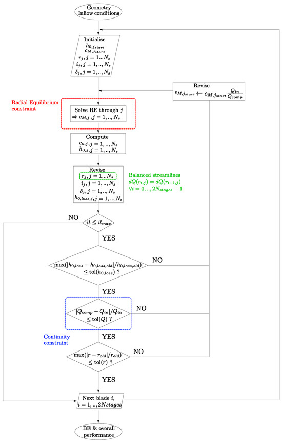
Figure 3.
Flow chart of ARES meanline solver.
- The computational domain is initialized at constant radial intervals, into which geometrical parameters and inflow boundary conditions are interpolated using a 3-point Lagrange technique.
- Meridional velocity spanwise distribution is evaluated at the first computing station.
- BE radial locations are updated along with the variables defined spanwise, including the empirical correlations.
- Convergence is checked according to maximum iterations and residual thresholds. Three criteria requiring simultaneous achievement are selected: the continuity with the inflow flow rate and residuals on both the BE radius locations and the head losses distribution, the latter referred to the previous iteration.
- Upon convergence, the code either moves to the next blade row or exits, thus printing the machine’s global and local statistics.
2.4. Empirical Correlations
Several correlations are included to model flow effects otherwise neglected by the assumptions adopted to solve the steady inviscid governing equations. The overall head losses are given as follows:
where the phenomenon-specific coefficients denote, respectively, profile losses, , secondary flows, , tip leakage, , and end-wall boundary layer (EWBL) effects, .
Concerning off-design behavior, the model assumes a dependency on the difference between the actual and reference incidence, . Thus, minimum loss profile losses and deviation are modified according to specific functions .
2.4.1. Minimum Loss Incidence
The parameter is modeled using Lieblein [10] measurements, from which the following correlation is derived:
Here, depends on the profile camberline shape, either Double Circular Arc (DCA) or NACA-65 equivalent; varies according to the profile thickness; is the reference incidence for a zero-camber, NACA 65-series, 10% thickness profile; and is the correlation slope. Coefficients definitions fitting the original data can be found in Aungier [20].
2.4.2. Deviation
The effective deviation, , is computed at any incidence starting from the minimum loss deviation, , with the latter defined according to Lieblein [10] as follows:
where is the parameter introduced above, depends on the profile thickness, is the reference deviation for a zero-camber, 65-series, 10% thickness aerofoil; and is the linear law slope. Coefficient correlations are proposed by Aungier [20]. The deviation is then computed by introducing additional effects as follows:
Here, models the planar cascades deviation at off-reference incidence following the theory by Dong-run et al. [21,22]; includes 3D flow dynamics based on Robbins et al. Johnson and Bullock [10]; and considers the impact of the Axial Velocity Ratio (AVR) across the cascades, which is modeled following Pollard and Gostelow [18].
2.4.3. Profile Losses
The profile losses at any operating condition rely on the minimum losses value, , which is modeled using the correlation by Lieblein [10]:
where and denote, respectively, the wake momentum thickness and the wake form factor. The correlations to close Equation (13) were modified by Koch and Smith [19] and recently rearranged by Tournier and El-Genk [15]. Thus, the effective loss parameter, , is modeled based on the incidence parameter, , by Aungier [20], where the correlations to compute are provided. Finally, the losses derive from the following:
2.4.4. Secondary Losses
Secondary flow losses are modeled using Herrig et al. [28] as expressed by Tournier and El-Genk [15]:
where is the average relative flow angle, and is the cascades lift coefficient.
2.4.5. Tip-Leakage Losses
In this case, the model adopted is the one proposed by Denton [29] as recently rearranged by Banjac et al. [16]. The theory directly relates the loss coefficient, , to the overall entropy production energy exchange, , associated to the leakage mass flow. The correlation reads as follows:
Here, a linear variation of the velocities across the tip profile is assumed. Thus, an integration is performed, including Lieblein [10] correlations, to obtain the entropy term.
2.4.6. End-Wall Boundary Layer Losses
External casing boundary layer losses are modeled following Howell [30], as proposed by Tournier and El-Genk [15]. The loss coefficient depends on the blade height, , and it is defined as follows:
Lumped models of the flow effects are linearly distributed along the blade radius. Table 2 summarizes the list of empirical correlations included in ARES.
Table 2.
Summary of the empirical correlations implemented.
3. Results and Discussion
Three test cases with available measurements from the literature are selected to asses the accuracy of the code. The corresponding primary parameters are reported in Table 3. It should be noted that, in the results discussion, the specific parameters follow the definitions of the corresponding reference papers. However, to facilitate the comparison among the case studies, the flow coefficient adopted in Table 3 is computed equivalently for any geometry and reads as follows:
where n is the rotational regime, D is the rotor external diameter, and Q is the volumetric flow rate.
Table 3.
Main parameters of the test cases adopted for the validation of ARES.
Before analyzing the code performance, the implementation was calibrated comparing empirical model combinations (Figure 4). Specifically, a sensitivity study was conducted to determine the minimum number of streamlines required to make the results independent of the channel discretisation. This investigation showed that incrementing above 21 does not provide consistent variation of the predicted statistics (Figure 4a), and therefore, this quantity was adopted henceforth. Thus, all the computations reach convergence below on all the residuals within 25 iterations. A typical residuals profile for near-design computations is reported in Figure 4b.
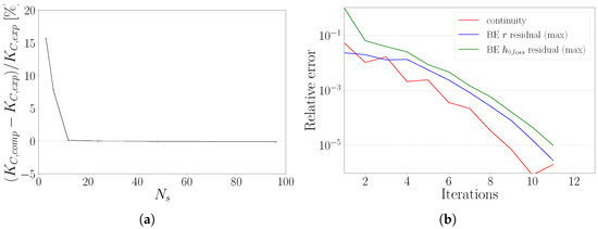
Figure 4.
Sensitivity analysis of the streamlines number, , (a) and typical convergence profile of a computation (b).
3.1. NASA Rotor 02
The NASA R02 is a straight-duct rotor intended for initial stages operations, following an inlet inducer. The geometry results from a modification of previous designs [32,33] and the blade element measurements were made available in Miller et al. [13]. The corresponding data are adopted as a reference for both the inflow boundary conditions and the outflow predictions comparison. Six different operating points (configurations 1 to 6) are selected within a range of flow coefficients, , ranging from to . Here, the machine parameter is defined as , with denoting the rotor passage cross-sectional area. For this case study, the inflow quantities are provided as radial profiles instead of uniform distributions.
The resulting rotor map is reported in Figure 5, depicting the work coefficient, , and the hydraulic efficiency, , as functions of the flow coefficient. Here, the two parameters are respectively defined as follows:
where the head is computed as the total pressure () jump across the rotor, is the tip rotor speed, and the ideal head rise is computed as .
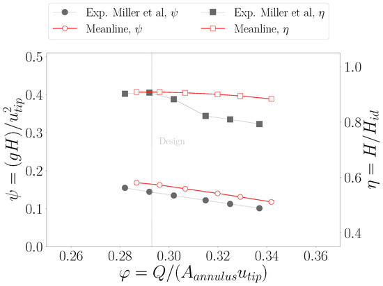
Figure 5.
Work coefficient and hydraulic efficiency as functions of the flow rate coefficient for the NASA R02 rotor, comparing ARES solution and experimental values from Miller et al. [13].
The pressure rise capability trend is in line with the experimental measurements. However, the computed solution exhibits a stable overprediction, inducing a discrepancy with a . However, with marginal improvements, the code portrays lower errors near the design operating conditions. This aspect is further emphasized by the efficiency curves comparison. In fact, from the experiments, the sudden drop of the hydraulic efficiency below the design point, combined with the smooth behavior of the work coefficient, suggests an abrupt increment of the measured torque. Differently, the code tends to smear out highly non-linear effects, recovering a smooth efficiency curve that constantly departs from the test data as the flow coefficient increases. As a result, the prediction error transitions from values below to over .
To investigate local accuracy, the spanwise distributions of meridional and tangential velocities and outflow relative angle are adopted to compare between ARES computations and experiments at both off- (configuration 1, ) and near-design (configuration 5, ) conditions (Figure 6).
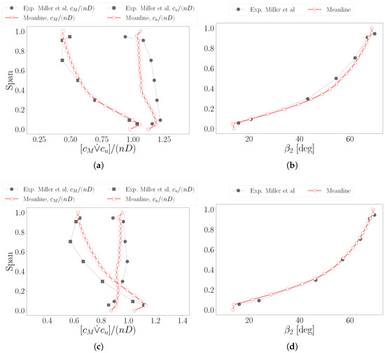
Figure 6.
Spanwise distributions of meridional and tangential velocities (left) and outflow relative angle (right) for off-design, , (a,b) and near-design, , conditions (c,d). Comparison between present computations and test data from Miller et al. [13].
For configuration 1, the tangential velocity distribution exhibits a significant alignment with the test data, except for a marginal discrepancy in the span region between and (Figure 6a). Conversely, the meridional component is stably underpredicted across the entire blade radius, with the major separation observed at mid-channel and the accuracy loss mitigated near the extremes. The mutual behavior of the two velocity components can be analyzed through the relative flow angle distribution (Figure 6b). The predicted curve is generally in good agreement with measurements, depicting a maximum of deviation above a span of . At this location, such overprediction is induced by the underprediction of , in contrast to the accurate estimate of . On the other hand, above a span of , the computed and measured curves tend to realign. This effect results from the underestimation of the tangential component, which is mitigated by a more accurate prediction of the meridional one.
The most accurate efficiency prediction is achieved for flow configuration 5. Since the computed head rise is higher than in the experiments, the low deviation of the efficiency curve depends on the ideal head rise prediction, which is a quantity uniquely determined by velocity components. In fact, the tangential velocity exhibits overprediction across the entire span, with a discrepancy increasing from the hub to shroud, except for end-wall boundary layer effects reducing the computed and tested curves separation (Figure 6c). The resulting meridional velocity prediction evidently suggests an accuracy improvement, despite a stable underestimation. Similarly to the previous case, the mid-channel solution exhibits higher deviation from the test data. Conversely, the relative flow angle portrays a significant alignment with experimental measurements, with further reduction of the discrepancy, now located near span (Figure 6d).
This analysis indicates that pressure and velocity predictions are not directly correlated. In fact, while flow directions were generally aligned with experiments, the pressure field was stably overpredicted.
3.2. HIREP
The HIgh REynolds number Pump (HIREP) facility was adopted to conduct measurements on the flow effects of an IGV installed upstream of a rotor [25,26]. Here, the test data between the two blades are retained as inflow boundary conditions, while computations are compared downstream of the rotor. This test case provides insights into the code accuracy, when operated under non-uniform, swirled inflow. An operating map is reconstructed, tracking the variation in the torque coefficient, , as a function of the flow coefficient, (Figure 7), with the former defined as in the reference experiments [25]:
where C is the rotor torque, and φ is defined as in Equation (18). Under near-design conditions, ARES exhibits significant accuracy. Conversely, the predicted maps depart from the experimental measurements, as off-design operations are considered. This behavior is more emphasized at higher values of , denoting a tendency to underestimate the rotor torque by up to . Differently, the discrepancy is reduced at lower values with a . The smooth monotonic trend of the curve is representative of the code stability over a wide range of operations.
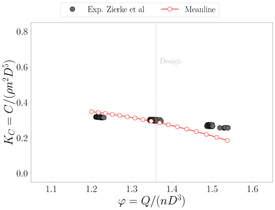
Figure 7.
Torque coefficient as a function of the flow rate coefficient for the HIREP rotor, comparing ARES solution and experimental values from Zierke et al. [25].
As local statistics, spanwise distributions of normalized velocities and pressure coefficients are considered at design condition (Figure 8). From the analysis of the tangential velocity component (Figure 8a) ARES can be seen to overpredict the flow turning, leading to negative values of . Differently, during experiments, this component was essentially suppressed downstream of the rotor. Thus, continuity forces the axial component to decrease, thereby producing the left-shift observable in the corresponding distribution. The total pressure curves underscore a tendency of the model to underestimate losses, depicting stably higher values than the test data (Figure 8b). However, the behaviour is not monotonic, with the greatest discrepancy occurring near midspan. Globally, the combination with the overprediction of the velocity distribution enables the model to recover a good agreement between the computed and measured static pressure fields. Anyhow, the curve is stably above experiments.
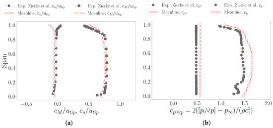
Figure 8.
Spanwise distribution of the flow statistics, comparing ARES solution and experiments from Zierke et al. [25], for design conditions (). Reported quantities include normalized tangential and axial velocities (a) and total and static pressure coefficients (b).
3.3. AxWJ-2
The test case represents a notional model for the validation of waterjet pump numerical models [27,31,34]. Here, the geometry is selected to evaluate the code accuracy for a rotor–stator configuration, featuring a shaped duct with a variable cross-sectional area. Computations are performed using uniform inflow boundary conditions derived from the processed mass flow rate.
In this case, the characteristic map reports the head rise coefficient, , and the hydraulic efficiency, , as functions of the flow coefficient, (Figure 9). While the latter follows Equation (18), the other two are defined below:
where the angular velocity expresses the rotational regime in rad/s.
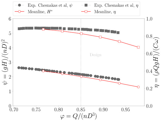
Figure 9.
Overall head coefficient and efficiency as functions of the flow rate coefficient for the AxWJ-2 pump, comparing ARES solution and experimental values from Chesnakas et al. [27].
ARES confirms significantly accurate near-design conditions (), with a discrepancy in the efficiency estimate, while exaggerating the head losses at higher mass flow rates. Despite keeping stable over a wide range of operating points, at low mass flow rates, the code diverges before completing the span of the experimental map. Notably, before the last simulated point, the results depict an increasing agreement with the reference measurements. Specifically, around the best efficiency point (), the efficiency is predicted with a error.
Thus, local Particle Image Velocimetry (PIV) measurements from Chesnakas et al. [27] are compared with computations at the station downstream of the rotor (Figure 10). In this case, the spanwise distribution of the axial velocity component (Figure 10a) significantly aligns with experiments, except for a velocity defect of the computed solution between the hub and of the span. Then, the present method exhibits difficulty in predicting boundary layer dynamics near the shroud, where it tends to preserve the lower span evolution. Similar considerations hold for the tangential velocity component (Figure 10b). In fact, for a major portion near the midspan, the numerical solution and test data are almost superimposed, while the lower and upper regions exhibit higher discrepancies. Especially for the latter, the results suggest scarce modeling of end-wall dynamics inside rotating domains.
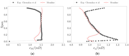
Figure 10.
Spanwise distribution of the flow statistics, comparing ARES solution and experiments from Chesnakas et al. [27] downstream of the AxWJ-2 rotor, for design conditions (). Reported quantities include normalized meridional (a) and tangential (b) velocities.
The same statistics are analyzed downstream of the stator blades (Figure 11). For this location, the disagreements are partially affected by the difference between the measurements station (at the nozzle exhaust) and the computations section (at the blade trailing edge), which differ due to the duct meridional shape variation. As a result, while the profile of the simulated axial velocity aligns with experiments (Figure 11a), the corresponding values are lower because the code does not model the additional downstream expansion. Furthermore, the computed hub dynamics emphasizes boundary layer evolution, inducing exaggerate spanwise fluctuations in the lower span. Considering the tangential velocity component, the difference between the two solutions is large (Figure 11b). While the wake dynamics impacts the evolution near the duct axis, the experiments exhibit an almost rectified flow. Differently, the numerical solution recovers a stably positive solution. Although the magnitudes are comparable between the computations and test data, the distribution profiles depict substantially different flow behaviors.
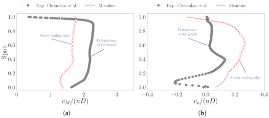
Figure 11.
Spanwise distribution of the flow statistics, comparing ARES solution and experiments from Chesnakas et al. [27] downstream of the AxWJ-2 stator, for design conditions (). Measurements refer to the nozzle exhaust, which further expands the flow from the station used for meanline predictions, at the blade trailing edge. Reported quantities include normalized meridional (a) and tangential (b) velocities.
The results for this case study align with the two previous investigations featuring a rotor-only configuration. The code demonstrates good accuracy in predicting the flow downstream of the rotating blades, whereas larger discrepancies arise when comparing the stator blade flow to experimental data.
4. Conclusions
ARES (Axial-flow pump Radial Equilibrium through Streamlines), a meanline code for designing axial-flow pumps for Outboard Dynamic-inlet Waterjets (ODW) applications, is introduced. The solver iteratively enforces flow momentum (aka Radial Equilibrium) and mass conservation laws to model the machine performance. In particular, several empirical correlations are adopted to model real-flow effects, such as off-design deviation, losses from profile shape, secondary flows, tip leakage, and the end-wall boundary layer (EWBL). A Blade Element Method (BEM) is used for the discretization process, addressing the meridional channel with planar cascades. This code is aimed at providing a fast and accurate tool for ODW axial-flow pump design. Specifically, the possibility to parameterize the geometry is a key ability that can be leveraged by optimization loops for the maximization of initial geometries performance.
The code’s accuracy is evaluated using three test cases: the NASA Rotor 02, the HIgh REynolds number Pump (HIREP), and the Axial-flow WaterJet pump (AxWJ-2). Global and local statistics compare the numerical solution to available experiments. The code is found to be stable over a wide range of operating points, with accuracy decreasing as the mass flow rate exceeded the design value. At lower values, the efficiency is predicted within a error compared to the test data, while at design conditions, the discrepancy exceeds . Spanwise distributions of the velocities and pressure generally show good agreement with measurements at the rotor exit. However, further calibration is needed to improve loss predictions near the hub and shroud walls, especially downstream of the stator blades.
Thus, this study is an intermediate step toward developing a comprehensive tool for Outboard Dynamic-inlet Waterjets (ODW) design. After further calibration, the research will integrate the pump module into the nacelle design routine for the meanline prediction of coupled operations. Integrated into an optimization algorithm, the code will be able to be exploited for accurate high-performance designs.
Author Contributions
Conceptualization, F.A., F.D.V. and A.M.; methodology, F.A., F.D.V. and A.M.; software, F.A.; validation, F.A.; formal analysis, F.A.; investigation, F.A.; resources, F.A. and E.B.; data curation, F.A., F.D.V. and A.M.; writing—original draft preparation, F.A., F.D.V. and A.M.; writing—review and editing, F.D.V., A.M. and E.B.; visualization, F.A.; supervision, F.D.V., A.M. and E.B.; project administration, E.B.; funding acquisition, E.B. All authors have read and agreed to the published version of the manuscript.
Funding
This research was funded by the University of Padova through the project ECO-SPEED, which was co-funded by SEALENCE S.p.a., under the program UNI-IMPRESA 2022.
Data Availability Statement
The original contributions presented in this study are included in the article. Further inquiries can be directed to the corresponding author.
Conflicts of Interest
The authors declare no conflict of interest.
Abbreviations
The following abbreviations are used in this manuscript:
| AVR | Axial Velocity Ratio |
| BE | Blade Element |
| BEM | Blade Element Method |
| CFD | Computational Fluid Dynamics |
| DCA | Double Circular Arc |
| EWBL | End-Wall Boundary Layer |
| HIREP | High Reynolds Number Pump |
| IGV | Inlet Guide Vane |
| ODW | Outboard Dynamic-inlet Waterjet |
| PIV | Particle Image Velocimetry |
| RE | Radial Equilibrium |
References
- Benini, E.; Gobbo, W. Propulsion Device with Outboard Waterjet for marine Vehicles. U.S. Patent 12,116,096, 15 October 2024. [Google Scholar]
- Avanzi, F.; De Vanna, F.; Magrini, A.; Benini, E. Numerical characterisation of Outboard Dynamic-inlet Waterjets: Propulsive aspects of intake/pump integration. Acta Mech. 2024. [Google Scholar] [CrossRef]
- Park, W.G.; Yun, H.S.; Chun, H.H.; Kim, M.C. Numerical flow simulation of flush type intake duct of waterjet. Ocean Eng. 2005, 32, 2107–2120. [Google Scholar] [CrossRef]
- Jung, K.H.; Kim, K.C.; Yoon, S.Y.; Kwon, S.H.; Chun, H.H.; Kim, M.C. Investigation of turbulent flows in a waterjet intake duct using stereoscopic PIV measurements. J. Mar. Sci. Technol. 2006, 11, 270–278. [Google Scholar] [CrossRef]
- Suryanarayana, C.; Satyanarayana, B.; Ramji, K.; Saiju, A. Experimental evaluation of pumpjet propulsor for an axisymmetric body in wind tunnel. Int. J. Nav. Archit. Ocean Eng. 2010, 2, 24–33. [Google Scholar] [CrossRef]
- Suryanarayana, C.; Satyanarayana, B.; Ramji, K.; Nageswara, M.R. Cavitation studies on axi-symmetric underwater body with pumpjet propulsor in cavitation tunnel. Int. J. Nav. Archit. Ocean Eng. 2010, 2, 185–194. [Google Scholar] [CrossRef]
- Shi, S.; Tang, W.; Huang, X.; Dong, X.; Hua, H. Experimental and numerical investigations on the flow-induced vibration and acoustic radiation of a pump-jet propulsor model in a water tunnel. Ocean Eng. 2022, 258, 111736. [Google Scholar] [CrossRef]
- Jiang, J.; Ding, J.; Lyu, N.; Luo, H.; Li, L. Control volume determination for submerged waterjet system in self-propulsion. Ocean Eng. 2022, 265, 112594. [Google Scholar] [CrossRef]
- Menegozzo, L.; Benini, E. Meanline Calculation of Surge Margin Loss due to Inlet Flow Distortion. In Proceedings of the Turbo Expo: Power for Land, Sea, and Air, Virtual, 21–25 September 2020; Volume 2A. [Google Scholar] [CrossRef]
- Johnson, I.A.; Bullock, R.O. Aerodynamic Design of Axial-Flow Compressors; Technical Report NASA-SP-36; NASA: Washington, DC, USA, 1965. Available online: https://ntrs.nasa.gov/api/citations/19650013744/downloads/19650013744.pdf (accessed on 3 March 2025).
- Henderson, R.E.; McMahon, J.F.; Wislicenus, G.F. A Method for the Design of Pumpjets; Technical Report NOw 63-0209-C-7; Pennsylvania State Univ State College Ordnance Research Lab: State College, PA, USA, 1964; Available online: https://apps.dtic.mil/sti/pdfs/AD0439631.pdf (accessed on 3 March 2025).
- Serovy, G.; Kavanagh, P.; Okiishi, T.; Miller, M. Prediction of Overall and Blade-Element Performance for Axial-Flow Pump Configurations; Technical Report NASA CR-2301; NASA: Washington, DC, USA, 1973. Available online: https://ntrs.nasa.gov/api/citations/19730023457/downloads/19730023457.pdf (accessed on 3 March 2025).
- Miller, M.J.; Okiishi, T.H.; Serovy, G.K.; Sandercock, D.M.; Britsch, W.R. Summary of Design and Blade-Element Performance Data for 12 Axial-Flow Pump Rotor Configurations; Technical Report NASA-TN-D-7074; NASA: Washington, DC, USA, 1973. Available online: https://ntrs.nasa.gov/api/citations/19730006255/downloads/19730006255.pdf (accessed on 3 March 2025).
- Furuya, O.; Chiang, W.L. A New Pumpjet Design Theory; Technical Report N00014-85-C-0050; David Taylor Research Center: Bethesda, MD, USA, 1988; Available online: https://apps.dtic.mil/sti/pdfs/ADA201353.pdf (accessed on 3 March 2025).
- Tournier, J.; El-Genk, M.S. Axial flow, multi-stage turbine and compressor models. Energy Convers. Manag. 2010, 51, 16–29. [Google Scholar] [CrossRef]
- Banjac, M.; Petrovic, M.V.; Wiedermann, A. Secondary Flows, Endwall Effects, and Stall Detection in Axial Compressor Design. J. Turbomach. 2015, 137, 051004. [Google Scholar] [CrossRef]
- Banjac, M.; Petrovic, M.V. Development of Method and Computer Program for Multistage Axial Compressor Design: Part I—Mean Line Design and Example Cases. In Proceedings of the Turbo Expo: Power for Land, Sea, and Air, Oslo, Norway, 11–15 June 2018; Volume 2C. [Google Scholar] [CrossRef]
- Pollard, D.; Gostelow, J.P. Some Experiments at Low Speed on Compressor Cascades. J. Eng. Power. 1967, 89, 427–436. [Google Scholar] [CrossRef]
- Koch, C.C.; Smith, L.H., Jr. Loss Sources and Magnitudes in Axial-Flow Compressors. J. Eng. Power. 1976, 98, 411–424. [Google Scholar] [CrossRef]
- Aungier, R.H. Axial-Flow Compressors: A Strategy for Aerodynamic Design and Analysis; ASME Press: New York, NY, USA, 2003. [Google Scholar]
- Wu, D.; Teng, J.; Qiang, X.; Feng, J. An Implicit Off-Design Deviation Angle Correlation of Axial Flow Compressor Blade Elements. In Proceedings of the Turbo Expo: Power for Land, Sea, and Air, Charlotte, NC, USA, 26–30 June 2017; Volume 2B, p. V02BT41A005. [Google Scholar] [CrossRef]
- Wu, D.; Teng, J.; Qiang, X.; Zheng, T. Development of an off-design deviation angle prediction model for full blade span in axial flow compressors. Proc. Inst. Mech. Eng. Part G J. Aerosp. Eng. 2019, 233, 3170–3183. [Google Scholar] [CrossRef]
- Guo, J.; Zhang, Y.; Chen, Z.; Feng, Y. CFD-based multi-objective optimization of a waterjet-propelled trimaran. Ocean Eng. 2020, 195, 106755. [Google Scholar] [CrossRef]
- Avanzi, F.; Baù, A.; De Vanna, F.; Benini, E. Numerical Assessment of a Two-Phase Model for Propulsive Pump Performance Prediction. Energies 2023, 16, 6592. [Google Scholar] [CrossRef]
- Zierke, W.C.; Straka, W.A.; Taylor, P.D. The High Reynolds Number Flow Through an Axial-Flow Pump; Technical Report TR 93-12; Applied Research Laboratory: Ferguson Township, PA, USA, 1993; Available online: https://apps.dtic.mil/sti/pdfs/ADA273844.pdf (accessed on 3 March 2025).
- Zierke, W.C.; Straka, W.A. Flow visualization and the three-dimensional flow in an axial-flow pump. J. Fluids Eng. 1996, 12, 250–259. [Google Scholar] [CrossRef]
- Chesnakas, C.J.; Donnelly, M.J.; Pfitsch, D.W.; Becnel, A.J.; Schroeder, S.D. Performance Evaluation of the ONR Axial Waterjet 2 (AxWJ-2); Technical Report NSWCCD-50-TR-2009/089; Naval Surface Warfare Center Carderock Division: Bethesda, MD, USA, 2009; Available online: https://apps.dtic.mil/sti/pdfs/ADA516369.pdf (accessed on 3 March 2025).
- Herrig, L.J.; Emery, J.C.; Erwin, J.R. Systematic Two-Dimensional Cascade Tests of NACA 65-Series Compressor Blades at Low Speeds; Technical Report NACA-TN-3916; NASA: Washington, DC, USA, 1957. Available online: https://ntrs.nasa.gov/api/citations/19930084843/downloads/19930084843.pdf (accessed on 3 March 2025).
- Denton, J.D. The 1993 IGTI Scholar Lecture: Loss Mechanisms in Turbomachines. J. Turbomach. 1993, 115, 621–656. [Google Scholar] [CrossRef]
- Howell, A.R. Fluid Dynamics of Axial Compressors. Proc. Inst. Mech. Eng. 1945, 153, 441–452. [Google Scholar] [CrossRef]
- Michael, T.J.; Schroeder, S.D.; Becnel, A.J. Design of the ONR AxWJ-2 Axial Flow Water Jet Pump; Technical Report NSWCCD-50-TR-2008/066; Naval Surface Warfare Center Carderock Division: Bethesda, MD, USA, 2008; Available online: https://apps.dtic.mil/sti/pdfs/ADA489739.pdf (accessed on 3 March 2025).
- Crouse, J.E.; Soltis, R.F.; Montgomery, J.C. Investigation of the Performance of an Axial-Flow-Pump Stage Designed by the Blade-Element Theory: Blade-Element Data; Technical Report NASA-TN-D-1109; NASA: Washington, DC, USA, 1961. Available online: https://ntrs.nasa.gov/api/citations/19980228119/downloads/19980228119.pdf (accessed on 3 March 2025).
- Miller, M.J.; Crouse, J.E.; Sandercock, D.M. Summary of Experimental Investigation of Three Axial-Flow Pump Rotors Tested in Water. J. Eng. Power. 1967, 89, 589–599. [Google Scholar] [CrossRef]
- Marquardt, M.W. Summary of Two Independent Performance Measurements of the ONR Axial Waterjet 2 (AxWJ-2); Technical Report NSWCCD-50-TR-2011/016; Naval Surface Warfare Center Carderock Division: Bethesda, MD, USA, 2011; Available online: https://apps.dtic.mil/sti/tr/pdf/ADA540499.pdf (accessed on 3 March 2025).
Disclaimer/Publisher’s Note: The statements, opinions and data contained in all publications are solely those of the individual author(s) and contributor(s) and not of MDPI and/or the editor(s). MDPI and/or the editor(s) disclaim responsibility for any injury to people or property resulting from any ideas, methods, instructions or products referred to in the content. |
© 2025 by the authors. Licensee MDPI, Basel, Switzerland. This article is an open access article distributed under the terms and conditions of the Creative Commons Attribution (CC BY) license (https://creativecommons.org/licenses/by/4.0/).