Abstract
Accurate modelling of carbon dioxide (CO2) dispersion and infiltration into buildings is essential for assessing the risks associated with accidental releases from carbon capture, utilisation, and storage (CCUS) infrastructure. This study presents an integrated analytical and computational framework for evaluating CO2 infiltration, incorporating a modified equation of state (EOS) to account for non-ideal gas behaviour. The original infiltration model, based on wind- and buoyancy-driven ventilation, is extended using a virial EOS. Key performance metrics are used to validate the model against experimental data and computational fluid dynamics (CFD) simulations. A comprehensive set of 30 case studies is used to assess model performance across a range of building geometries and environmental conditions. Results show that the modified EOS has minimal impact on far-field predictions, confirming the robustness of the ideal gas assumption under ambient conditions. Importantly, the study finds that CO2 impurities do not significantly affect far-field dispersion once ambient pressure is reached, though they may influence near-field behaviour at the release point.
1. Introduction
At standard conditions, carbon dioxide (CO2) is a colourless, odourless gas which is denser than air and undetectable by human senses. The current average atmospheric concentration of CO2 exceeds 400 ppm [1]. However, in high concentrations CO2 is an asphyxiant and can have toxic effects above 4% by volume [2]. Furthermore, due to its high density, CO2 will displace air at ground level and, depending on environmental conditions, can accumulate in topographic dips and depressions such as valleys. CCUS schemes involve large quantities of CO2 and it is imperative that the associated risk is appropriately managed. A release of CO2 from CCUS infrastructure, including pipelines, could cause severe consequences for nearby populations if not properly managed.
Following a pipeline rupture, the CO2 will begin to depressurise to atmospheric pressure. This could involve a phase change to the gaseous and solid phases. The initial outflow is momentum-driven because of the significant pressure difference between the CO2 contained in the pressurised pipeline and its surroundings. Once expanded, the CO2 will disperse at atmospheric pressure depending on environmental conditions. Due to its high Joule–Thomson expansion coefficient, the expanding CO2 can cool to temperatures lower than 273 K and it will condense the water in the surrounding air and form a visible white plume. During this, cooling particles of solid CO2 can form which will be carried in the jet. The white plume gives an indication of the concentration of CO2 to levels of 1% by volume [3] which is lower than levels that cause harmful effects.
To assess the risks surrounding onshore CO2 pipeline transportation, Quantitative Risk Assessment (QRA) procedures can be put in place. The procedure involves calculating the probability of failure and the consequences of failure and using them to determine the individual and societal risks. To determine the consequences of failure, the dispersion behaviour of CO2 and the infiltration rate of a plume of CO2 into buildings are needed. Following a release of CO2, people in the vicinity of the release will move away from the release and potentially seek shelter from the plume. The CO2 plume could drift towards buildings, causing the concentration of CO2 inside these buildings to increase as CO2 enters through windows, doors, and adventitious openings. The amount of accumulation of CO2 inside the buildings is key to the safety of their occupants. In [4], an analytical shelter model based on wind- and buoyancy-driven ventilation was created which can be used to predict the effect of carbon dioxide exposure on building occupants following a release from an onshore CO2 pipeline. The model can be used as part of a QRA process for a CO2 pipeline to calculate the level of exposure of CO2 to the surrounding population along with a CO2 leakage and dispersion models such as [5,6].
This study introduces a novel enhancement to the analytical model of [4] by incorporating a virial equation of state (EOS), offering a more accurate representation of non-ideal gas behaviour. Key performance metrics, including peak concentration and dosage, are used to validate the model against experimental and CFD data.
1.1. Previous Models
The analytical model [4] works on the principle of natural ventilation where flow is driven by wind and buoyancy effects caused by pressure differences between the inside of the building and its surroundings and temperature differences within the building. The model extends [7] by combining both wind- and buoyancy-driven ventilation mechanisms in the manner of Etheridge and Sandberg [8,9]. Alongside the analytical model, a computational fluid dynamics (CFD) CO2 infiltration model was also created using STAR-CCM+ [10] with the Reynolds-Averaged Navier–Stokes (RANS) equations. The CFD model uses the same inputs as the analytical model (CO2 concentration and temperature external to the enclosure) and can predict the rate of CO2 accumulation in an enclosure engulfed by a plume of CO2.
The models were validated against a test of CO2 infiltration into an enclosure; full details of the test are given in [4,11] but a brief summary is provided here. Experimental measurements of CO2 accumulation within the enclosure were taken as a cloud of drifting CO2 passed the enclosure following a scaled pipeline rupture experiment that was conducted as part of the National Grid COOLTRANS research programme [12]. The average wind speed was 1.17 m/s during the release and the wind was incident on the front face of the enclosure at an angle of approximately 20 degrees from the normal. The enclosure was 3.5 m by 3.5 m and 3 m high with metal sheet sides, a roof, and no internal partitions. It was sealed apart from two openings. One opening was 1.04 m high by 0.24 m wide and positioned upwind and the other opening was 1.04 m high by 0.22 m wide and positioned downwind. The height from the floor to the bottom of the windows was 1.3 m.
The ventilation rate (in terms of air changes per hour) into the enclosure was much higher than would be expected for a typical domestic house. This was to allow a measurable quantity of CO2 to build up inside the enclosure during the timescale of the experiment.
1.2. Analytical Model Details
Ventilation in the model is due to buoyancy and temperature effects. The pressure difference between inside and outside at a height z, denoted , is given by
where Csp is a surface pressure coefficient, and are the pressure of the external and internal fluids, Uwind is the incident wind speed, P’ is a pressure determined by the location of the zero-pressure level, and g is gravitational acceleration.
The volumetric flow rate at a height z through an opening, Q(z), is then calculated using
where Cd is a discharge coefficient, W(z) is the width of the opening at a height z, and ρ is fluid density.
Total flow in, Qin, and total flow out, Qout, are calculated using Simpson’s rule, following
respectively, where z0 is the neutral pressure level, the height where the internal and external pressures are equal, and h is the height of the building.
Densities are calculated using the ideal gas law and by assuming that the air and CO2 are perfectly mixed. The change in internal concentration, Cint, in a time step dt, then, is
where and are the external and internal volume concentrations of CO2, respectively, and Vb is the volume of the enclosure.
The change in internal temperature is determined by assuming ideal gas behaviour, conservation of mass, perfect mixing inside the enclosure, and that the specific heat capacities of CO2 and air are roughly equal, which leads to
where Tint is the temperature inside the enclosure and Text is the temperature of the fluid outside the enclosure.
The process is solved iteratively for P′ with the condition of steady state flow. At each time step, the internal concentration and temperature are updated. Using this procedure, it is possible to calculate the change in internal CO2 concentration over time. In the analytical model, the concentration of CO2 inside the enclosure is assumed to be uniform.
1.3. CFD Model Details
The CFD model solves the equations for continuity of mass, momentum, and energy, as well as chemical species. In the model, the humidity of the air is neglected and the air and CO2 mixture is treated as a single-phase fluid. The standard turbulence model [13] was corrected with the Lag Elliptic Blending (EB) model [14] to incorporate the effect of buoyancy-driven flows with low Reynolds number. A Computer-Aided Design (CAD) model was built to exactly replicate the experimental setup which was imported into Star-CCM+. A polyhedral mesh was chosen with 45,000 cells and a prism layer mesher was used in the near-wall regions. The setup used a maximum Courant–Friedrichs–Lewy (CFL) number of 10 and a mean CFL number of 5 over the whole domain. Any existing initial turbulence is ignored in the model.
1.4. Previous Findings
Comparisons were made between the analytical model, the CFD model, and experimental data for the build-up of CO2 in the enclosure and the changes in internal temperature.
The analytical and CFD models used the experimental average wind speed and direction as well as the geometry of the test enclosure as inputs into the models. The temperature and CO2 concentration at the inlet were used as the inputs to the models at a frequency of 1 s; these are shown in Figure 1 and Figure 2, respectively. The CFD model was identical to the test setup. However, the analytical model used the size of the upwind opening was used for both openings, i.e., the area of the downwind opening was oversized by around 8%.
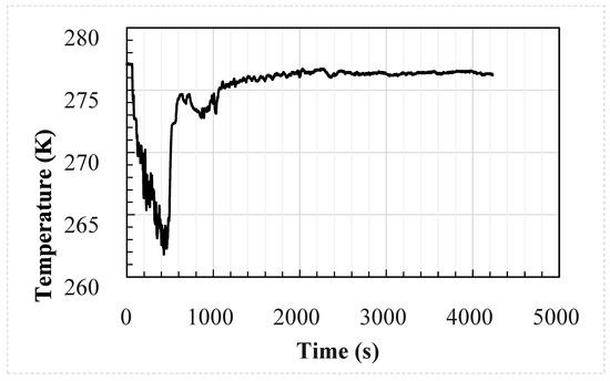
Figure 1.
Measured external temperature of the welding hut experimental setup.
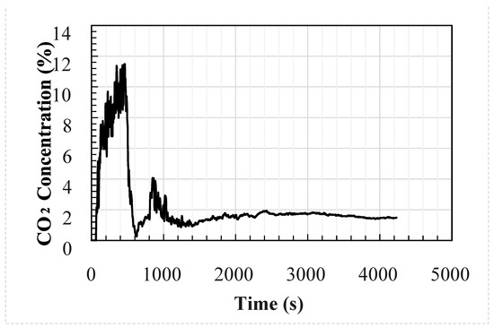
Figure 2.
Measured external concentration of the welding hut experimental setup.
In the analytical model values of the discharge coefficient, pressure coefficient at the upwind side of the enclosure and pressure coefficient at the downwind side of the enclosure were set at 0.61, 0.7, and −0.2, respectively, following [7]. A sensitivity analysis of these coefficients was conducted in [15], where 4800 combinations were tested across 30 representative building scenarios. The optimal set minimised deviation from CFD predictions, improving accuracy in peak concentration and short-term exposure limit timing. Notably, cases with low air changes per hour (ACHs), due to small window areas or low wind speeds, showed greater divergence between models, highlighting the importance of coefficient selection. These findings underscore the need for further experimental data to refine pressure coefficients specific to CO2 plumes.
The models then predicted the accumulation of CO2 in the enclosure over time. The models both produced very similar results and matched the experimental data well, although they tended to slightly over-predict the concentration of CO2 inside the enclosure. If used in a QRA, then the models would produce results which would be slightly conservative.
A broader evaluation of the analytical model’s applicability to residential-style building geometries and varied environmental conditions was conducted in [15]. This involved comparing its predictions with those from a CFD model across thirty representative scenarios. These test cases systematically varied key factors influencing CO2 ventilation, including wind speed, opening dimensions and placement, internal temperature, and building size. The results demonstrated strong agreement between the analytical and CFD models in predicting indoor CO2 accumulation.
2. Proposed Modifications to the Analytical Model
The original work by Lyons et al. [4], uses the ideal gas equation of state
where R is the gas constant and n is the number of mols of gas. Rewritten in terms of the mass density, ρ = nm/V, this becomes
where is the average molar mass, e.g., (here, and are molar masses of air and CO2, respectively).
We propose to replace this with the virial equation of state expanded with one term. That is,
where = n/V = ρ/m is the molar number density and B is the second virial coefficient term. Here, B provides the first order correction to the ideal gas law and B depends on both temperature and molecular composition. The molecular composition dependence is not required so this is deferred until needed. In contrast, the temperature dependence is needed almost immediately (i.e., when deriving the enthalpy change for gas entering the building). If a change in EOS is necessary, then replacing the ideal gas law with a first order virial expansion should give a large difference in the results of the model. Equation (9) can be rearranged to give a pressure explicit EOS.
or in terms of mass density,
2.1. Importance of the Additional Term at Standard Conditions
From the RHS of Equation (9), we can see that non-ideal gas behaviour is seen when B(T) becomes sufficiently close to 1 that it cannot be neglected. Using [16] as implemented in [17], at standard conditions for temperature and pressure for pure CO2, the density of is = 4.5 × 10⁻⁵ mol/cm3 and the second virial coefficient calculated is B = −152 cm3/mol, and so B(T) = −7 × 10⁻³. To demonstrate the impact of temperature fluctuations in the far field, we consider standard pressure conditions. A temperature change of and then leads to B(T) values of −5 × 10⁻² and −9 × 10⁻², respectively. Thus, these values illustrate that non-ideal gas behaviour is subtle in the far field, but its inclusion remains important for completeness and for identifying thresholds where deviations become significant under different conditions. In contrast, under near-field conditions (standard temperature and a pressure of 100 bar), B(T) reaches −150.3, and the deviation is highly significant.
2.2. Density Expression
The model of [4] requires a calculation of the internal and external gas densities and this is achieved by rearranging the ideal gas law for ρ (Equations (10) and (11) of [4]). A similar rearrangement of the virial equation can be achieved by applying the quadratic formula to Equation (11):
This expression replaces Equations (10) and (11) from [4]. Note, if is small then and hence the ideal gas law expression is recovered.
2.3. Change in Internal Energy Due to Expansion
When the gas enters the building, it changes density from ρext to ρint. As it is colder outside the building than inside, the gas will expand. This expansion will have to do work against the internal interactions of the gas (which are absent for an ideal gas), and this will lower internal energy.
We assume that the expansion happens isothermally at the external temperature Text (i.e., that work done on the surroundings does not change Text). The expression relating changes in internal energy, U, to changes in temperature and volume is
where Cv is the specific heat capacity at constant volume. Equation (10) with density replaced by volume is
Thus,
Substituting this into Equation (13) (with gives
The change in internal energy on expansion, , is then
where Vint and Vext are the volumes of gas inside and external to the building, respectively. The change in internal energy on expansion per mol is then
2.4. Change in Building Temperature Due to Gas Exchange
When nin is the mols of gas entering the building, the extra internal energy is
where is the molar specific heat capacity of the external gas and Text is the temperature of the gas outside the building. Thus, the change in internal energy is
For the gas exiting the building, the change in internal energy is
where and are the molar specific heat capacity and temperature of gas within the building and nout is the number of mols of gas leaving the building.
Hence the total change in internal energy is
In a steady state, . We assume , since is approximately the same for CO2 and air in this case (which is valid for small temperature differences), and where is the number of mols of gas inside the building. These give
As a last step, we replace the number of mols n with mass M to obtain
where Mbuild and Min are the masses of gas inside and entering the building, respectively. This is Equation (22) from [4], with the extra non-ideal term ∆uexp/cv. The expansion was assumed isothermal at to simplify the derivation and because the process occurs rapidly as the gas enters the building, limiting heat exchange. This assumption is consistent with the well-mixed approach used in [4], where . In reality, the expansion may be non-isothermal, which would increase the calculated internal energy change and slightly accelerate the predicted temperature rise. However, under far-field conditions, this effect is expected to be small. Future work could incorporate a non-isothermal treatment for near-field scenarios where temperature gradients are larger.
3. Testing the Analytical Model in Further Scenarios
In the original work by Lyons et al. [4], the ventilation rate into the enclosure was much higher than would be expected for a typical domestic house so that a measurable quantity of CO2 built up inside the enclosure during the timescale of the experiment. For this reason, to test the modifications to the model with buildings’ geometries more closely resembling domestic abodes and against a wider range of conditions, the 30 test cases from [15] were used.
3.1. Test Case Details
The main parameters affecting CO2 ventilation rate are wind speed, the area and height of the openings, internal temperature, and building height, width, and length. The ranges of the variables are shown in Table 1 and a schematic of the building is shown in Figure 3. The minimum width and length were chosen based on [18] which state that a single bedroom should be at least 2.15 m wide (rounded down to 2 m). The minimum height was based on UK building regulations which state that the minimum floor to ceiling height should be a minimum of 2.3 m (rounded down to 2 m) for at least 75% of the Gross Internal Area [18]. The minimum temperature was chosen to be 5 °C based on the boiler frost temperature of a typical boiler [19]. There is no maximum temperature for buildings in UK law; a maximum temperature of 20 °C based on the average maximum temperature for July across the UK based on data from the Met Office [20] was chosen. The wind range was chosen based on the Beaufort wind force scale and range from a light breeze to a violent storm. Maximum sizes, the range of opening areas, and the heights of the beginnings of openings were estimated based on the project team’s experience of buildings around the UK.

Table 1.
Range of the 30 case study inputs.
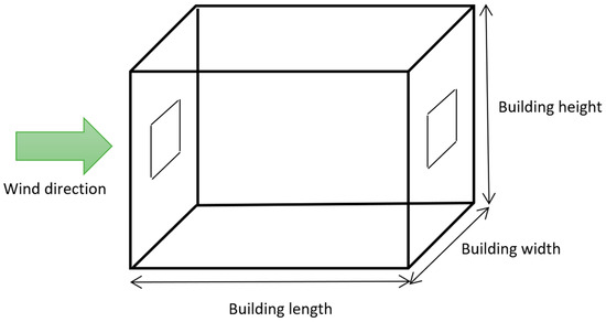
Figure 3.
Schematic of the building.
From the ranges of the variables, a set of 30 test cases were generated using a maximum Latin hypercube design to ensure an even spread in the parameter space. The cases are shown in Table 2.
Table 2.
Details of the 30 cases.
3.2. Test Case Conditions
For ease of comparison, each of the models used the same input of external temperature and external concentration for all 30 case studies. A higher profile for the concentration of CO2 and a longer duration were chosen compared to the experimental setup to allow for greater testing of the models. The same external temperature and concentrations were used as inputs for each case in both models.
The profiles were generated using an in-house flat terrain dispersion model created by DNV-GL developed from the results of COOLTRANS experiments [11,21] and are shown in Figure 4 and Figure 5. A double-ended guillotine break type rupture is assumed to occur at the mid-point of a 96 km long dense phase CO2 pipeline and the valve closure is set to 15 min after the start of the release. The temperature of the CO2 in the pipeline is assumed to be 30 °C and the wind speed 5 m/s. The CO2 cloud dispersion was modelled for two hours following the rupture. Details of the pipeline parameters which remain constant between each simulation are provided in Table 3. The wind was assumed to be blowing directly onto the face of the enclosure, and the building was located 100 m from the release.
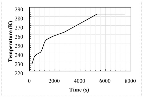
Figure 4.
External temperature used as input for the 30 case studies.
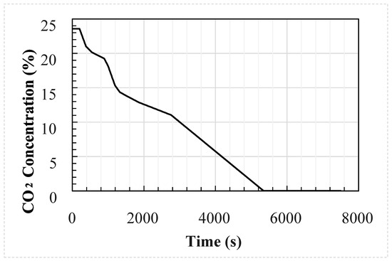
Figure 5.
External concentration used as input for the 30 case studies.
Table 3.
Dispersion model inputs.
Using the concentration and temperature inputs from above, the models were then run for each of the thirty cases to generate the change in internal CO2 concentration over time.
3.3. CFD Model for the Test Cases
The CFD model setup, including boundary conditions and mesh independence testing, follows the methodology described in Lyons et al. [4]. The same CAD geometry, boundary conditions (e.g., no-slip walls, atmospheric outlet pressure, incompressible flow), and turbulence model (Lag EB k-ε) were used. A mesh convergence study was previously conducted using coarse (45 k), medium (110 k), and fine (300 k) meshes, with no significant improvement observed beyond the coarse mesh. Therefore, the coarse mesh was adopted for all simulations, and the mesh of an example case is shown in Figure 6.
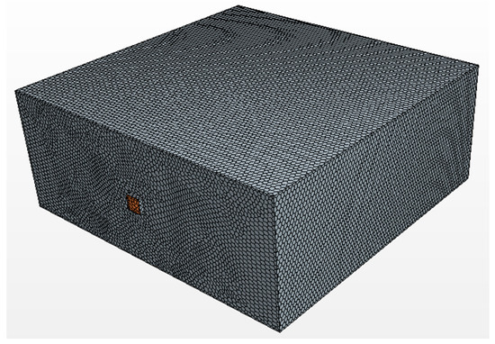
Figure 6.
Example of the mesh of the CFD model for one of the cases. The openings are shown in yellow.
The values were updated for each case following Table 2. To generate an average concentration from the CFD models (needed for comparison to the analytical model), CO2 measurements were averaged from the sensors placed inside the building, which were 5 cm apart in vertical planes and were in line with the windows and covered the cross section of the building, as in Figure 7.
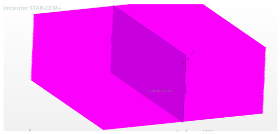
Figure 7.
Example of the placement of CO2 sensors in the CFD model.
4. Results and Discussion
The modified analytical model was compared with the previous model and to the experimental data set using the input conditions of [4]. The set of 30 representative case studies was used to compare the results of the modified analytical model to data generated by the original analytical and CFD models. To evaluate the performance of the models in reproducing the experimental and CFD results, three key prediction metrics were identified:
- The peak concentration reached in a case.
- The time to reach the peak concentration of a case.
- The integral of the concentration over the length of time of the release (the area under the time/concentration plot) corresponding to the dosage of CO2 received.
These were selected on the basis that the cumulative effect of CO2 concentration is the most important parameter for safety, as limiting the exposure to CO2 over time is the primary driver for a risk analysis. The time to reach the peak concentration and the value of the peak concentration were selected since the higher the concentration of CO2 received was, the more dangerous to life it was. To calculate the dosage received, an order 6 polynomial regression was performed on the concentration/time data to generate a curve which was then integrated over the period of the release to find the area under the graph.
4.1. Comparison of the Models with Experimental Data
The modified analytical model was compared to the experimental data set using the identified key parameters. The comparison can be seen in Table 4, along with the results of the original analytical and CFD models. For the areas under the concentration/time curve, the R2 values for the regressions of the experimental data, analytical model, modified analytical model, and CFD model are 0.897, 0.905, 0.905, and 0.897, respectively. As can be seen, the differences between the analytical and modified analytical models are very small. The dosages (related to the area under the regression) over the period of the simulation are within 0.08% of each other; the modified analytical model reaches the peak concentration 32 s sooner and the peak concentration values are within 0.09%.
Table 4.
Comparison between the models and experimental data of the key infiltration parameters for the welding hut case.
Figure 8 shows a comparison between the average values of the internal CO2 concentration predicted using both analytical shelter models and the data recorded during the experimental test case. As shown in the figure, the results of the analytical models are indistinguishable, and both reproduce the experimental data to a good degree.
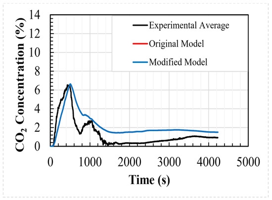
Figure 8.
Experimental and computed internal concentrations for the welding hut.
4.2. Comparing the Analytical and CFD Models over the 30 Case Studies
Table 5 shows the values of the identified parameters for the original analytical, modified analytical, and CFD models for each of the 30 cases. For the areas under the curves, the CFD regression R2 have values between 0.963 and 1.000, and the analytical models’ regression R2 values lie between 0.968 and 1.000.
Table 5.
Comparison between the models of the key infiltration parameters for the 30 cases.
The predictions of the analytical models are almost identical. Looking at the peak concentrations, all results lie within 0.3% of each other and the modified analytical model has higher peak concentrations for all case studies except Case 3. The times to reach the peak concentration are identical for all the case studies. Comparing the integrals under the regressions, the results of the modified analytical model are within 0.4% of those of the analytical model. Again, the results of the modified analytical model are higher except for Case 3. Since there is greater variation in the integral area (0.4% versus 0.3%), this means that the concentration predictions of the models differ across time by varying amounts. However, the results are so close that the differences between the results of the model are insignificant.
Across all the cases, most of the analytical integrals are within 3% of the CFD integrals. Case 16 shows the largest difference between the analytical and CFD integrals, where the analytical integral is 21% higher than the CFD integral. The other cases outside of 3% are Case 10 and Case 12, where the analytical integrals are 6% and 16% lower than the CFD integral, respectively. The peak concentration predictions show greater variance between the models. Here, a total of 10 cases show a deviation of 10% or more between the predictions of the models. The analytical model underpredicts the peak concentration compared to the CFD model except in Cases 15, 16, 21, and 22. Cases 6, 16, and 30 show the largest deviations between the models (21%, 19%, and 20%, respectively). Apart from Case 23, the analytical model predicts a shorter time to reach the short-term exposure limit of CO2. The values look quite different with Cases 1, 3, 6, 12, 13, 16, and 30 showing a factor of 2 difference between the predictions of the model. However, both models predict that the short-term exposure limit is reached within 5 min and the only cases that differ by more than 100 s are Cases 6 and 12. The only case that the CFD model predicts a longer time to reach the short-term exposure limit for is Case 23, where it predicts that the limit is reached 2 s after the prediction by the analytical model.
Overall, the analytical models are able to reproduce the results of the CFD model to a reasonable degree. They tend to disagree for small window areas and low wind speeds which may be caused by a low rate of air change. This is supported by [9], “when pressures generated by wind are negligible then ventilation flow rate calculations have the highest level of uncertainty”.
4.3. Implications of the Similarity Between Results
Since the results of the modified and analytical models are almost identical, this means that the ideal gas law, which is used as the EOS in the original analytical model, is sufficient for modelling the ingress of CO2 at ambient pressure coming from a cloud outside a shelter, and no modification to the equation of state used in the analytical model is necessary. To further explain this similarity, it is important to note that the analytical model’s predictions are primarily driven by ventilation parameters rather than the EOS. A comprehensive sensitivity analysis of discharge and pressure coefficients was presented in Wetenhall et al. [15], where results showed that coefficient tuning can improve accuracy under low-ACH conditions.
Further implications of this result are that the addition of impurities in the CO2 stream will have no effect on ventilation once ambient pressure has been reached by the mixture, i.e., only the external pressure and temperature are needed and the mixture will make no difference since the ideal gas law does not differentiate between substances.
This means that in the far field, once a mixture has fully decompressed, then impurities do not need to be considered. However, it is important to note that in the near field impurities will affect density (and calculations) much more and so must be included in any analysis.
5. Conclusions
The EOS in the analytical model of [4] was replaced with the virial equation of state expanded with one term. The results of the modified analytical model were compared to a set of experimental data and model results from CFD and the original analytical model. The results indicate the following:
- There is good agreement between the experimental data and the outputs of the models.
- The analytical models reproduce the CFD results reasonably well.
- There is little difference between the results of the modified and original analytical models. No modification to the EOS used in the analytical model is necessary, and the ideal gas law produces sufficiently accurate results.
- The findings support the use of the ideal gas law for far-field modelling but highlight the need for more detailed EOS in near-field, high-pressure conditions.
- Any impurities added to the CO2 stream will make negligible differences to the ventilation results once ambient pressure is reached.
- The assumption that the CO2 and air mix perfectly is a sound one.
Future Work
Current CO2 ventilation models are based on models using ambient air; in particular, all the pressure coefficients used in these models are for air. A cloud of CO2 from a pipeline rupture will behave differently to air since it is much cooler than ambient air and thus will show very different buoyancy effects.
There is a need for CO2 ventilation testing under a variety of wind directions and speeds and different building/opening geometries to determine the pressure coefficients specifically for CO2. Future work should also explore the impact of the building geometry and ventilation configurations on infiltration dynamics under varying atmospheric conditions. With these data, models can give more accurate predictions of CO2 ventilation into shelters.
This study focused on pure CO2 and far-field conditions, where the composition dependence of the second virial coefficient was negligible. However, this assumption limits the generality of the model for near-field scenarios or mixtures containing impurities such as N2, O2, or CH4. In such cases, mixture-specific virial coefficients and cross-interaction terms become important and could influence density and energy calculations. Future work should also incorporate mixture effects to extend the applicability of the model to real pipeline compositions and high-pressure conditions immediately downstream of a rupture.
Author Contributions
Conceptualization, B.W., R.S.G., C.J.L. and J.M.R.; methodology, B.W., R.S.G., C.J.L. and B.A.; formal analysis, B.W.; investigation, B.W., N.R. and B.A.; writing—original draft preparation, B.W.; writing—review and editing, B.W., R.S.G., J.M.R., B.A. and N.R.; supervision, B.W. and J.M.R.; project administration, B.W.; funding acquisition, B.W. and R.S.G. All authors have read and agreed to the published version of the manuscript.
Funding
This research was funded by the UKCCSRC Scientific Collaboration Fund under EPSRC EP/P026214/1.
Institutional Review Board Statement
Not applicable.
Informed Consent Statement
Not applicable.
Data Availability Statement
The raw data supporting the conclusions of this article will be made available by the authors on request. However, restrictions apply to the availability of the experimental data used in the study, which were provided by National Grid and DNV-GL.
Acknowledgments
The authors would like to thank the UKCCSRC for providing the funding for the study and National Grid and DNV-GL for the provision of the experimental data used in the study.
Conflicts of Interest
Author Chris J. Lyons was employed by the company Pipeline Integrity Engineers. The remaining authors declare that the research was conducted in the absence of any commercial or financial relationships that could be construed as a potential conflict of interest.
References
- Team, E.W. ESRL Global Monitoring Division-Global Greenhouse Gas Reference Network. Trends in Atmospheric Carbon Dioxide; Global Monitoring Laboratory: Boulder, CO, USA, 2019. [Google Scholar]
- Health & Safety Executive. Toxicity Levels of Chemicals: Assessment of the Dangerous Toxic Load (DTL) for Specified Level of Toxicity (SLOT) and Significant Likelihood of Death (SLOD); Health & Safety Executive: Bootle, UK, 2015. [Google Scholar]
- Wen, J.; Heidari, A.; Xu, B.; Jie, H. Dispersion of carbon dioxide from vertical vent and horizontal releases—A numerical study. Proc. Inst. Mech. Eng. Part E J. Process Mech. Eng. 2013, 227, 125–139. [Google Scholar] [CrossRef]
- Lyons, C.; Race, J.; Adefila, K.; Wetenhall, B.; Aghajani, H.; Aktas, B.; Hopkins, H.; Cleaver, P.; Barnett, J. Analytical and computational indoor shelter models for infiltration of carbon dioxide into buildings: Comparison with experimental data. Int. J. Greenh. Gas Control 2020, 92, 102849. [Google Scholar] [CrossRef]
- Shao, Y.; Cao, X.; You, W.; Zhao, S.; Nan, Z.; Biang, J. Far-Field Behavior of Supercritical CO2 Being Dispersed Due to Leakage from Pipelines. Fluid Dyn. Mater. Process. 2024, 20, 2867–2885. [Google Scholar] [CrossRef]
- Wang, H.; Liu, B.; Liu, X.; Lu, C.; Deng, J.; You, Z. Dispersion of carbon dioxide released from buried high-pressure pipeline over complex terrain. Environ. Sci. Pollut. Res. 2021, 28, 6635–6648. [Google Scholar] [CrossRef] [PubMed]
- BS5925; 1991 Code of Practice for Ventilation Principles and Designing for Natural Ventilation. British Standards Institute: London, UK, 1991; p. 1991.
- Etheridge, D.W.; Sandberg, M. A simple parametric study of ventilation. Build. Environ. 1984, 19, 163–173. [Google Scholar] [CrossRef]
- Etheridge, D.W.; Sandberg, M. Building Ventilation: Theory and Measurement; John Wiley and Sons: New York, NY, USA, 1996. [Google Scholar]
- Siemens. SP Software, STAR-CCM+; Siemens: Munich, Germany, 2016. [Google Scholar]
- Lyons, C.J.; Race, J.M.; Hopkins, H.F.; Cleaver, P. Prediction of the consequences of a CO2 pipeline release on building occupants. In Proceedings of the 25th Institution of Chemical Engineers Symposium on Hazards 2015 (HAZARDS 25), Edinburgh, UK, 13–15 May 2015; pp. 235–245. [Google Scholar]
- Allason, D.; Armstrong, K.; Barnett, J.; Cleaver, P.; Halford, A. Experimental studies of the behaviour of pressurised releases of carbon dioxide. In Proceedings of the 23rd Institution of Chemical Engineers Symposium on Hazards, Southport, UK, 12–15 November 2012; pp. 142–152. [Google Scholar]
- Launder, B.E.; Sharma, B.I. Application of the energy-dissipation model of turbulence to the calculation of flow near a spinning disc. Lett. Heat Mass Transf. 1974, 1, 131–137. [Google Scholar] [CrossRef]
- Revell, A.J.; Benhamadouche, S.; Craft, T.; Laurence, D. A stress-strain lag Eddy viscosity model for unsteady mean flow, International. Int. J. Heat Fluid Flow 2006, 27, 821–830. [Google Scholar] [CrossRef]
- Wetenhall, B.; Race, J.M.; Adeflia, K.; Aktas, B.; Aghajani, H.; Lyons, C.; Reppas, N. Suitability and optimisation of analytical indoor shelter model used for infiltration of carbon dioxide for typical dwellings. In Proceedings of the 16th Greenhouse Gas Control Technologies Conference (GHGT-16), Lyon, France, 23–24 October 2022. [Google Scholar]
- Span, R.; Wagner, W. A New Equation of State for Carbon Dioxide Covering the Fluid Region from the Triple-Point Temperature to 1100 K at Pressures up to 800 MPa. J. Phys. Chem. Ref. Data 1996, 25, 1509–1596. [Google Scholar] [CrossRef]
- Lemmon, E.W.; Bell, I.H.; Huber, M.L.; McLinden, M.O. NIST Standard Reference Database 23: Reference Fluid Thermodynamic and Transport Properties-REFPROP, Version 10.0; Standard Reference Data Program; National Institute of Standards and Technology: Gaithersburg, MD, USA, 2018. [Google Scholar]
- Department for Communities and Local Government. Technical Housing Standards—Nationally Described Space Standard; Department for Communities and Local Government: London, UK, 2015. [Google Scholar]
- Ideal. User Guide Ideal Instinct 24; Ideal: East Yorkshire, UK, 2017; pp. 30–35. [Google Scholar]
- Met Office. Mean Daily Maximum Temperature—August Average: 1981–2010; Met Office: Exeter, UK, 2010. [Google Scholar]
- Barnett, J.; Cooper, R. The COOLTRANS Research Programme: Learning for the Design of CO2 Pipelines. In Proceedings of the 2014 10th International Pipeline Conference IPC2014, Calgary, AB, Canada, 29 September–3 October 2014. [Google Scholar]


Disclaimer/Publisher’s Note: The statements, opinions and data contained in all publications are solely those of the individual author(s) and contributor(s) and not of MDPI and/or the editor(s). MDPI and/or the editor(s) disclaim responsibility for any injury to people or property resulting from any ideas, methods, instructions or products referred to in the content. |
© 2025 by the authors. Licensee MDPI, Basel, Switzerland. This article is an open access article distributed under the terms and conditions of the Creative Commons Attribution (CC BY) license (https://creativecommons.org/licenses/by/4.0/).