Article

A Novel Subgrid Model Based on Convection and Liutex

Department of Mathematics, The University of Texas at Arlington, Arlington, TX 76019, USA
*
Author to whom correspondence should be addressed.
Fluids 2025, 10(11), 292; https://doi.org/10.3390/fluids10110292
Submission received: 18 October 2025 / Revised: 6 November 2025 / Accepted: 7 November 2025 / Published: 11 November 2025
(This article belongs to the Special Issue Vortex Definition and Identification)

Abstract

This paper proposes a novel convention-based subgrid scale (SGS) model for large eddy simulation (LES) by using the Liutex concept. Conventional SGS models typically rely on the eddy viscosity assumption, which uses the linear eddy viscosity terms to approximate the nonlinear effects of unresolved turbulent eddies, that should be measured by unresolved Liutex. However, the eddy viscosity assumption is empirical but lacks a scientific foundation, which limits its predictive accuracy. The proposed model in this paper directly models the convective terms and demonstrates several key advantages: (1) the new model gets rid of isotropic assumption for the unresolved SGS eddies which are, in general, anisotropic, (2) the new model contains no empirical coefficients which need to be adjusted case by case, (3) the new model explicitly captures nonlinear convective effects by the SGS eddies and (4) the new model is consistent with the physics for boundary layer as the model becomes zero in the laminar sublayer, where Liutex becomes zero automatically. This new model has been applied in the flat plate boundary transition flow, and the results show that it outperforms the popular and widely adopted wall-adapting local eddy (WALE) model. This new model is a conceptual breakthrough in SGS modeling and has the potential to open a new direction for more accurate SGS models and future LES applications.

1. Introduction

Large eddy simulation (LES) with a subgrid scale (SGS) model has been introduced for a long time. LES was first proposed in 1963 by Joseph Smagorinsky [1] to simulate atmospheric air currents, and later first explored by Deardorff [2]. LES is widely applied in various engineering fields, including combustion [3], acoustics [4] and simulations of the atmospheric boundary layer [5]. In the Smagorinsky model [1], the influence of the SGS motions is represented through an eddy viscosity concept given by Boussinesq’s eddy viscosity assumption [6].
τ i j 1 3 δ i j τ k k = 2 ν t S ¯ i j
where τ i j represents the SGS stresses, S ¯ i j refers to large-scale strain-rate tensor, and ν t is the Smagorinsky model’s eddy viscosity, which can be expressed as
ν t = C s Δ 2 2 S ¯ i j S ¯ i j
where C s is an adjustable coefficient and Δ is a characteristic length scale. Following Smagorinsky’s pioneering work, numerous eddy-viscosity models have been proposed by subsequent researchers. Some widely used SGS models have been developed, including the wall-adapting local eddy (WALE) model [7], the dynamic Smagorinsky model [8], the Vreman model [9] and the anisotropic minimum-dissipation (AMD) model [10]. In 2022, Ding, Wang et al. [11] published a new SGS model by using Liutex which is the first subgrid model that uses Liutex. The eddy viscosity becomes zero in the laminar sublayer automatically without any artificial adjustment in Ding-Wang model.
Vortices, which are synonymous with eddies, play a crucial role in LES modeling. Liutex [12,13,14], a third generation vortex definition and identification method, was introduced by Liu et al. in 2018 as a mathematical definition of vortex. Wang et al. [15] derived an explicit formula for computing the magnitude of Liutex. The expression of Liutex R can be written as
R = R r = [ ω · r ω · r 2 4 λ c i 2 ] r
where ω represents the vorticity vector, r indicates the local rotational axis and is the real eigenvector of v and λ c i is the imaginary part of the complex conjugate eigenvalue of v .
The concept of Liutex has the following significant advantages over the previous vortex identification methods, such as the Q criterion [16], λ 2 criterion [17], etc. First, Liutex is derived purely from kinematics, making it applicable to all types of flows, e.g., compressible flow and incompressible flow, which is independent of any dynamics. Second, Liutex is a vector which provides both local rotational axis and rotation strength. All existing vortex identification criteria are scalers which cannot be applied to define a vortex. Third, Liutex avoids the contamination of shear or stretching [18]. In addition, the physical meaning of Liutex is very clear, which shows the local rotation axis and the exact angular speed of the fluid rotation, while others are scalers and their physical meanings are not clear. We cannot use a scalar to define a vector in principle.
Although many SGS models have been proposed, none of them jump out of the framework introduced by Smagorinsky in which eddy viscosity is adopted to reflect the influence of SGS motions. This paper proposes a revolutionary SGS model by directly modifying convective terms. Since the primary effect of SGS eddies is to alter the convective quantity, the proposed convection-based SGS model more accurately captures the physical essence of SGS eddies than traditional eddy viscosity formulations. This is the first time that a Liutex and convection based SGS model has been proposed, and the new model is a groundbreaking concept for SGS study. This paper is organized as follows: Section 2 explains the limitations of eddy-viscosity SGS models; Section 3 introduces the newly proposed convection- and Liutex-based SGS model; Section 4 presents its application; and a summary is given in Section 5.

2. Limitations of Eddy Viscosity

In previous SGS models, eddy viscosity is introduced to account for the effects of SGS eddies, as these eddies enhance momentum transport in a manner which is like molecular viscosity. However, this analogy has several limitations.
1.
Eddy viscosity does not capture the essential effect of SGS eddies.
Although both SGS eddies and viscosity can enhance momentum transport, their mechanisms are fundamentally different. SGS eddies transport momentum through convection, whereas viscosity contributes via diffusion. Equation (4) presents the filtered momentum equation in the Navier–Stokes equations.
u ¯ i t + x j u ¯ i u ¯ j = p ¯ x i τ i j x j + 1 R e 2 u ¯ i x i x j
τ i j = u i u j ¯ u ¯ i u ¯ j
where · ¯ represents the result after filtering. In Equation (4), the residual SGS stress term τ i j , which is modeled in previous LES models, is derived from filtering the convective term x j u i u j in the original momentum equation. Consequently, eddy viscosity is an empirical approximation of the momentum transport caused by SGS eddies through convection.
2.
Eddy viscosity uses linear terms to approximate nonlinear terms.
In conventional SGS models, the Boussinesq hypothesis is adopted, which assumes a linear relation between the residual SGS stress term τ i j and the filtered rate of strain S ¯ i j . τ i j is nonlinear since u i u j ¯ and u ¯ i u ¯ j are products of velocity components, while S ¯ i j is linear because the exponent of u ¯ is 1 in S ¯ i j = 1 2 u ¯ + u ¯ T . One distinct difference is the frequency. Suppose u = s i n y , then the convective term u u y becomes
u u y = 2 s i n y · c o s y = s i n 2 y
Here, the angular frequency is doubled through the nonlinear process. In contrast, a linear approximation preserves the original frequency and cannot create any higher frequencies. Thus, using linear terms to analogize the nonlinear convective effects, as in previous SGS models, can limit their accuracy.
3.
Viscosity is a physical property of molecules.
Viscosity is an intrinsic physical property of molecules and is independent of the eddy strengths. Eddy viscosity is merely an empirical approximation made in the absence of a better alternative. There is no mechanism that fluid viscosity can be changed by vortex or turbulence mixing.

3. Convection-Based SGS Model

The accurate velocity vector V can be written as
V = v + v
where v represents the resolved numerical solution obtained from computation and v represents the unresolved small length scales or residuals. Then, accordingly,
V = v + v
where V represents the accurate velocity gradient, v is the numerical solution and v is the unresolved part of V . Compared with v , v is a higher order error since v is the partial derivative of v and taking a derivative will reduce the order of accuracy or, in other words, the error created by v is an order larger than the error created by v . Therefore, v is neglected in building the new model and v + v v + v v v + v . W e   o n l y   n e e d   t o   m o d e l   v .
According to Liu’s triple decomposition [19,20], V can be decomposed into rotation, stretching/compression and shear parts, which can be written as
v = R o r + S C + S
R o r = 0 R z 2 R y 2 R z 2 0 R x 2 R y 2 R x 2 0
where R o r , S C and S are defined as the rotation, stretching/compression and shear parts, respectively, and R x , R y and R z are the components of Liutex vector R in x, y and z directions, respectively. Similarly, v can be decomposed as
v = Ror + SC + S
where R o r , S C and S are the error of rotation, stretching/compression and shear parts, respectively. Since eddies dramatically influence the convection inside the grids, R o r or small eddies are dominant in the unresolved scales as the shear and stretching functions are smoother. Here only R o r is considered in building this model. So,
V = v + v v + R o r u x u y u z v x v y v z w x w y w z + 0 R z 2 R y 2 R z 2 0 R x 2 R y 2 R x 2 0
Equation (12) is the correction that the new model makes after taking R o r into account. The above formula can be rewritten in scalar form as follows:
U y = u y R z 2                U z = u z + R y 2
V x = v x + R z 2                V z = v z R x 2
W x = w x R y 2                W y = w y + R x 2
U x = u x         V y = v y         W z = w z
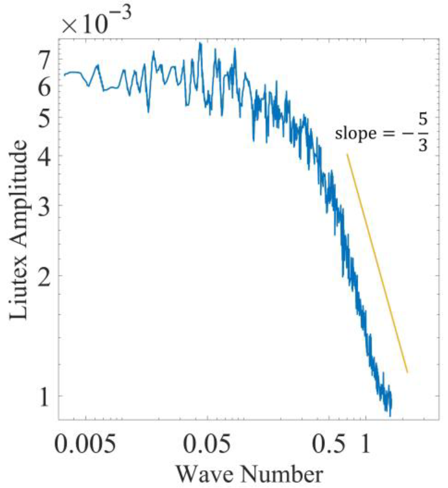
Figure 1 shows a sketch of the turbulence energy spectrum. In LES, a cutoff wave number κ c separates the resolved and unresolved motions. Motions with smaller wave numbers are resolved while those with larger wave numbers are unresolved. If the spectrum and κ c are known, then the ratio of unresolved motions to resolved motions can be estimated. Similarly, R x , R y and R z can be evaluated based on the cutoff wave number and Liutex similarity. Liutex has been found to be satisfied with the 5 3 law [21,22,23], as illustrated in Figure 2.
According to the Nyquist–Shannon sampling theorem [24,25], κ c has the following relation with the gap between two adjacent grid points:
κ c = π d
where d represents the distance between two adjacent grid points. Let E R κ denote the Liutex spectrum function. The ratio of unresolved Liutex to resolved Liutex is
C κ c = u n r e s o l v e d r e s o l v e d = κ c E R κ d κ 0 κ c E R κ d κ
So, for one dimension, unresolved R can be computed from resolved R by
R = C κ c R
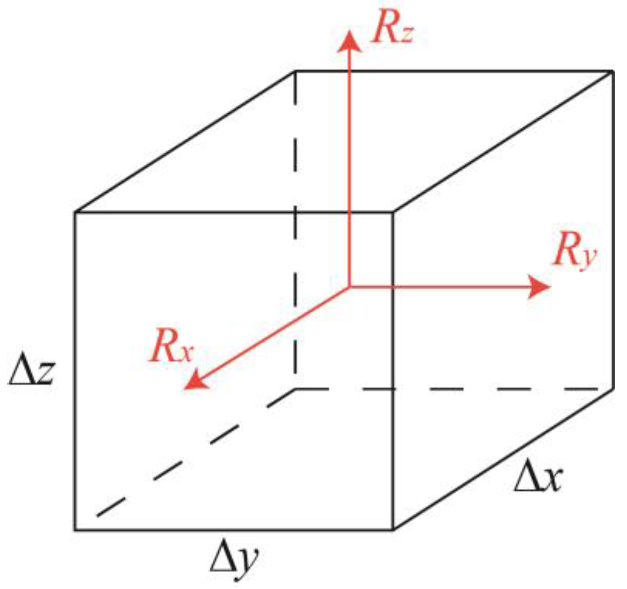
Figure 3 shows a grid cell whose dimensions are Δ x , Δ y and Δ z with three components of Liutex R x , R y and R z . Once the rotational axis is fixed, the rotation occurs in a two-dimensional plane which is orthogonal to the axis. Δ x Δ y is chosen to estimate the cutoff wave number for the x-y plane (corresponds with R z ) and the same approach is applied to x-z and y-z planes. The cutoff wave number for R x , R y and R z are
κ c x = π Δ y Δ z ,            κ c y = π Δ x Δ z ,            κ c z = π Δ x Δ y
And unresolved R x , R y and R z can be calculated by
R x = C κ c x R x
R y = C κ c y R y
R z = C κ c z R z
The original momentum equation in x direction is
u t + u u x + v u y + w u z = 1 ρ p x + τ x x x + τ y x y + τ z x z + g x
τ x x = 2 3 μ 2 u x v y w z
τ y x = μ u y + v x
τ z x = μ u z + w x
Considering the corrections to u y , u z , v x , w x and substituting Equations (13)–(16) into Equations (24)–(27), the equations become
u t + u u x + v u y R z 2 + w u z + R y 2 = 1 ρ p x + τ x x x + τ y x y + τ z x z + g x
τ x x = 2 3 μ 2 u x v y w z
τ y x = μ u y R z 2 + v x + R z 2 = μ u y + v x
τ z x = μ u z + R y 2 + w x R y 2 = μ u z + w x
where R y and R z can be evaluated by Equations (22) and (23). Modifications are marked in red. One can find that the corrections to the stress expressions cancel each other in Equations (30) and (31).
Similarly, the momentum equations in y and z directions of the proposed new model are
v t + u v x + R z 2 + v v y + w v z R x 2 = 1 ρ p x + τ x y x + τ y y y + τ z y z + g y
w t + u w x R y 2 + v w y + R x 2 + w w z = 1 ρ p x + τ x z x + τ y z y + τ z z z + g z
with no modifications to the expressions of τ y y , τ x y , τ z y , τ x z , τ y z and τ z z in the original Navier–Stokes equations. Modifications, marked in red, are only made in Equations (28), (32) and (33), which form the revised momentum equations in the proposed new model. Applying the above procedure, one can find that the continuity equation and energy equation in the proposed new model remain the same as the original ones in the Navier–Stokes equations.
The proposed new SGS model has the following theoretical merits:
  • The proposed model modifies the convective terms, capturing the physical essence that unresolved eddies enhance momentum transport by convection.
  • Unlike all other SGS models, there is no empirical coefficient in the proposed model. All expressions are derived theoretically.
  • The proposed model is anisotropic. Unresolved vortices have rotation axes which have directions, so a good SGS model should not be isotropic.

4. Application and Results

The proposed model is tested in the case of the boundary layer transition on a flat plate with a Mach number 0.5 [26,27]. Compressible Navier–Stokes equations are solved in the simulation. A sixth-order compact scheme is used for spatial discretization and a third-order Runge–Kutta method is implemented for time marching. Two-dimensional and three-dimensional Tollmien–Schlichting waves are enforced at the inlet boundary. Periodic boundary conditions are used at the spanwise boundary, while non-slip conditions are used at the wall boundary. Non-reflecting boundary conditions are set at both the outlet boundary and far field boundary. In this simulation, the Mach number is set as 0.5, the Reynolds number R e = ρ u δ i n μ is chosen to be 1000, where δ i n is the inflow displacement thickness. L x = 988.658 δ i n and L y = 22 δ i n are the lengths of the computation domain in streamwise and spanwise directions, respectively. L z i n = 40 δ i n represents the height of the computation domain at the inlet. Figure 4 shows the computation domain. Two sets of mesh are used, which are 1920 × 128 × 241 (G1) and 480 × 32 × 60 (G2). Simulations without any models are performed on G1 (regarded as a direct numerical simulation (DNS) result) and G2. The proposed model is tested on G2. The WALE model is also applied on G2 as a comparison.
The expression of the WALE model [7] is
ν t = C w Δ 2 S i j d S i j d 3 / 2 S ¯ i j S ¯ i j 5 / 2 + S i j d S i j d 5 / 4
S i j d = 1 2 g ¯ i j 2 + g ¯ j i 2 1 3 δ i j g ¯ k k 2
g ¯ i j = u ¯ i x j ,        g ¯ i j 2 = g ¯ i k g ¯ k j
where S ¯ i j represents the resolved rate of strain and Δ is the grid scale and defined as Δ x Δ y Δ z 3 in this simulation. C w is the model coefficient and chosen to be 0.325, which has been found to be suitable for a wide range of flows in ANSYS Fluent and is widely used [28,29,30].
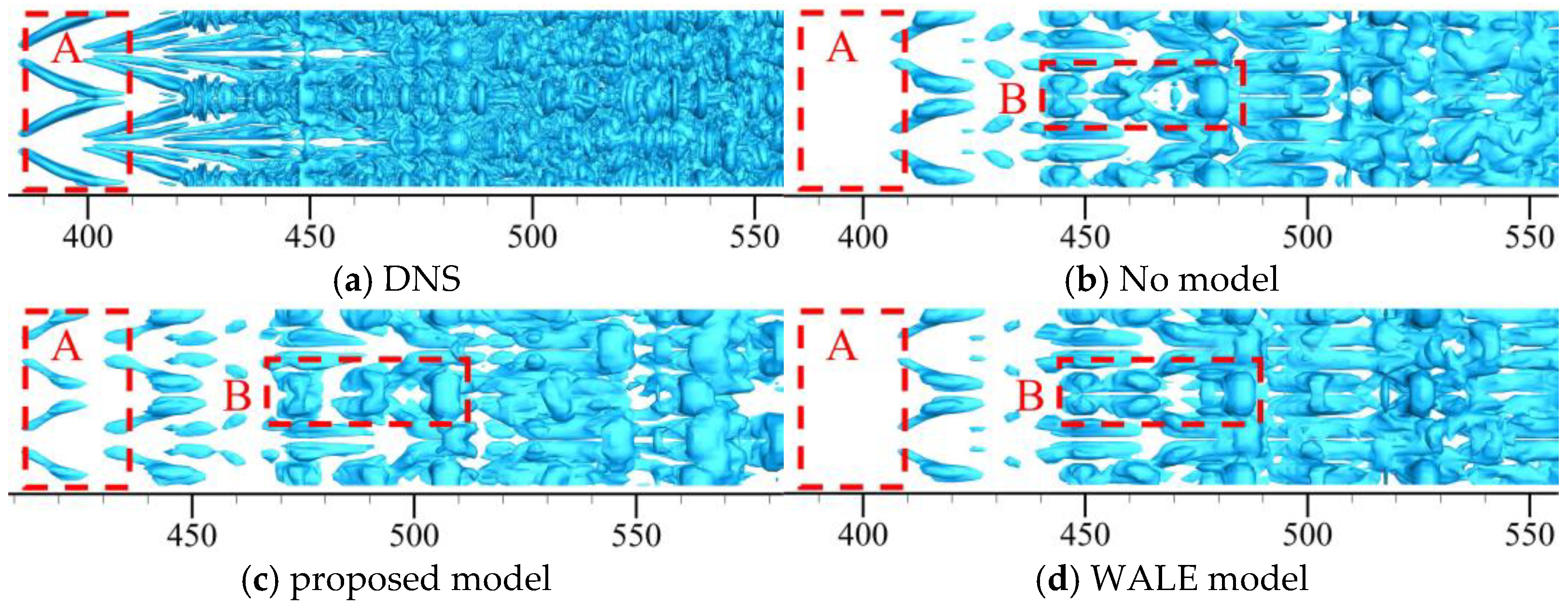
The comparison of vortex structures, represented by Lituex iso-surface, for different models and grids is presented in Figure 5. The iso-surface threshold is chosen to be 0.015 for all cases. Due to the coarser resolution, Figure 5b–d exhibit less detail than Figure 5a. In region A, the proposed model successfully resolves the first λ vortex, while the no model and the WALE model cases do not. In region B, the proposed model clearly shows the formation of three vortex rings, while the vortex rings shown in the no model and WALE model cases are not complete. Generally, the proposed model captures more vortex structures than the no model and WALE model.
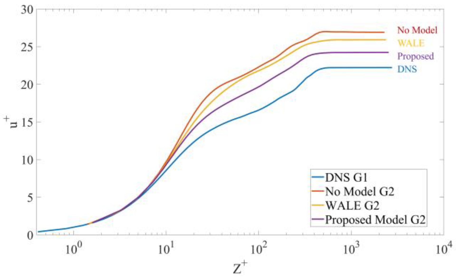
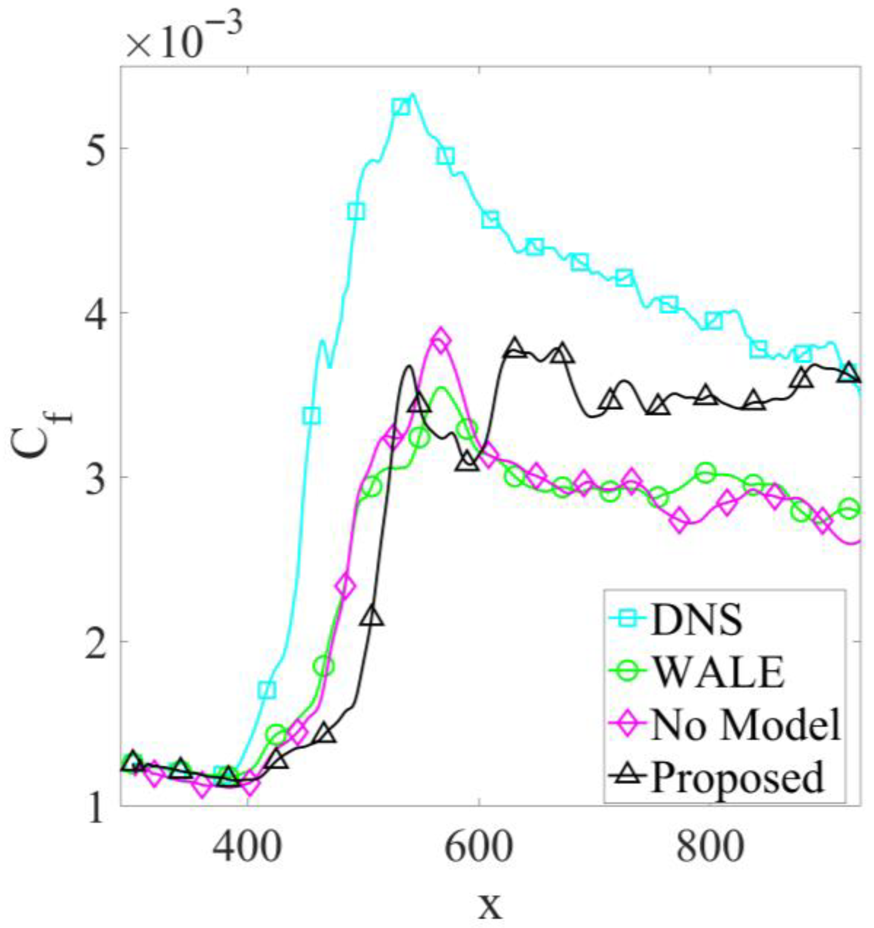
Figure 6 shows the time- and spanwise-averaged velocity profile on grid G2 at x = 800 , normalized by wall units, for the WALE model, the proposed model and the no model cases. The DNS result is also drawn as a standard. Due to using only 1 64 of the DNS grid numbers, the curve of no model deviates noticeably from the DNS result. The WALE model slightly improves the result while the proposed model shows dramatic improvements. The proposed model’s curve lies approximately midway between the no model and the DNS results, which shows the currently proposed model is two times better than the popular WALE SGS model. Figure 7 provides the comparison of the no model, WALE and the proposed model against the DNS data for the prediction of normalized and spanwise-averaged Reynolds stress components, including u + u + ¯ , v + v + ¯ , w + w + ¯ , u + w + ¯ . For u + u + ¯ , all models behave similarly, showing higher values than the DNS result in the near wall region and then the curves drop rapidly to below the DNS curve. The peak of the proposed model lies between those of the no model and WALE model. For v + v + ¯ , the proposed model is the only one whose profile can go up to the same peak level as the DNS result, while the peaks of the WALE model and no model are approximately 75% of the DNS peak. For w + w + ¯ and u + w + ¯ , the proposed model is also noticeably closer to the DNS curve than the other two approaches. The time- and spanwise-averaged skin friction coefficient ( C f ) distributions along the streamwise direction for different approaches are shown in Figure 8. As expected, the DNS curve is higher than the other approaches, representing the fully resolved turbulent behavior. The no model and WALE model both underpredict C f across most of the domain, reflecting insufficient resolution. The proposed model shows a notable improvement over both WALE and no model results. The curve of the proposed model is notably closer to the DNS curve and higher than the curves of WALE and no model in the post-transition region, indicating that the proposed model predicts more developed turbulence compared to the other two approaches.

5. Conclusions

This paper proposes, for the first time, an SGS model through modifying convective terms based on Liutex. Traditional SGS models based on eddy viscosity face several key limitations. Traditional SGS models approximate nonlinear convective effects using a linear eddy viscosity and depend on empirical coefficients. In addition, traditional SGS models approximate the anisotropic effects of unresolved eddy with an isotropic eddy viscosity concept. In contrast, the proposed convection-based SGS model directly modifies the convective terms by Liutex and Liutex similarity, which are inherently anisotropic and nonlinear, and contain no empirical parameters. When applied to a flat plate boundary layer transition case, the new model exhibits significantly improved performance over the WALE model in predicting the mean velocity profile, Reynolds stress components and mean skin friction coefficients. This new convective term modeling by Liutex represents a conceptual breakthrough and has the potential to redefine LES research.

Author Contributions

Conceptualization, Y.Y. and C.L.; methodology, Y.Y.; writing—original draft preparation, Y.Y.; writing—review and editing, C.L.; initiative and advice, C.L.; funding acquisition, Y.Y. and C.L. All authors have read and agreed to the published version of the manuscript.

Funding

This research was funded by US NSF, grant number 2422573 and grant number 2300052.

Institutional Review Board Statement

Not applicable.

Informed Consent Statement

Not applicable.

Data Availability Statement

The raw data supporting the conclusions of this article will be made available by the authors on request.

Acknowledgments

The authors are grateful to the Texas Advanced Computing Center (TACC) for providing computation resources. During the preparation of this manuscript/study, the author(s) used ChatGPT (https://chatgpt.com/) for the purpose of checking grammar and typos. The authors have reviewed and edited the output and take full responsibility for the content of this publication. This research is supported by the US NSF under grants #2300052 and # 2422573.

Conflicts of Interest

The authors declare no conflicts of interest.

Abbreviations

LESLarge eddy simulation
SGSSubgrid Scale
WALEWall-adapting local eddy
AMDAnisotropic minimum-dissipation
DNSDirect numerical simulation

References

  1. Smagorinsky, J. General circulation experiments with the primitive equations: I. The basic experiment. Mon. Wea. Rev. 1963, 91, 99–164. [Google Scholar] [CrossRef]
  2. Deardorff, J.W. A Numerical Study of Three-Dimensional Turbulent Channel Flow at Large Reynolds Numbers. J. Fluid Mech. 1970, 41, 453–480. [Google Scholar] [CrossRef]
  3. Pitsch, H. Large-eddy simulation of turbulent combustion. Annu. Rev. Fluid Mech. 2006, 38, 453–482. [Google Scholar] [CrossRef]
  4. Wagner, C.; Hüttl, T.; Sagaut, P. (Eds.) Large-Eddy Simulation for Acoustics, 1st ed.; Cambridge University Press: Cambridge, UK, 2007; ISBN 978-0-521-87144-0. [Google Scholar]
  5. Sullivan, P.P.; McWilliams, J.C.; Moeng, C.-H. A Subgrid-Scale Model for Large-Eddy Simulation of Planetary Boundary-Layer Flows. Bound.-Layer Meteorol. 1994, 71, 247–276. [Google Scholar] [CrossRef]
  6. Boussinesq, J. Essai Sur La Théorie Des Eaux Courantes; Impr. Nationale: Paris, France, 1877. [Google Scholar]
  7. Nicoud, F.; Ducros, F. Subgrid-Scale Stress Modelling Based on the Square of the Velocity Gradient Tensor. Flow Turbul. Combust. 1999, 62, 183–200. [Google Scholar] [CrossRef]
  8. Germano, M.; Piomelli, U.; Moin, P.; Cabot, W.H. A Dynamic Subgrid-Scale Eddy Viscosity Model. Phys. Fluids A Fluid Dyn. 1991, 3, 1760–1765. [Google Scholar] [CrossRef]
  9. Vreman, A.W. An Eddy-Viscosity Subgrid-Scale Model for Turbulent Shear Flow: Algebraic Theory and Applications. Phys. Fluids 2004, 16, 3670–3681. [Google Scholar] [CrossRef]
  10. Rozema, W.; Bae, H.J.; Moin, P.; Verstappen, R. Minimum-Dissipation Models for Large-Eddy Simulation. Phys. Fluids 2015, 27, 085107. [Google Scholar] [CrossRef]
  11. Ding, Y.; Pang, B.; Yan, B.; Wang, Y.; Chen, Y.; Qian, Y. A Liutex-Based Subgrid Stress Model for Large-Eddy Simulation. J. Hydrodyn. 2022, 34, 1145–1150. [Google Scholar] [CrossRef]
  12. Liu, C.; Gao, Y.; Tian, S.; Dong, X. Rortex—A New Vortex Vector Definition and Vorticity Tensor and Vector Decompositions. Phys. Fluids 2018, 30, 035103. [Google Scholar] [CrossRef]
  13. Liu, C.; Gao, Y.; Dong, X.; Wang, Y.; Liu, J.; Zhang, Y.; Cai, X.; Gui, N. Third Generation of Vortex Identification Methods: Omega and Liutex/Rortex Based Systems. J. Hydrodyn. 2019, 31, 205–223. [Google Scholar] [CrossRef]
  14. Wang, Y.; Gao, Y.; Xu, H.; Dong, X.; Liu, J.; Xu, W.; Chen, M.; Liu, C. Liutex Theoretical System and Six Core Elements of Vortex Identification. J. Hydrodyn. 2020, 32, 197–211. [Google Scholar] [CrossRef]
  15. Wang, Y.; Gao, Y.; Liu, J.; Liu, C. Explicit Formula for the Liutex Vector and Physical Meaning of Vorticity Based on the Liutex-Shear Decomposition. J. Hydrodyn. 2019, 31, 464–474. [Google Scholar] [CrossRef]
  16. Hunt, J.C.; Wray, A.A.; Moin, P. Eddies, Streams, and Convergence Zones in Turbulent Flows. Center for Turbulence Research Proceedings of the Summer Program. 1988. Available online: https://ntrs.nasa.gov/citations/19890015184 (accessed on 17 October 2025).
  17. Jeong, J.; Hussain, F. On the Identification of a Vortex. J. Fluid Mech. 1995, 285, 69–94. [Google Scholar] [CrossRef]
  18. Kolář, V.; Šístek, J. Stretching Response of Rortex and Other Vortex-Identification Schemes. AIP Adv. 2019, 9, 105025. [Google Scholar] [CrossRef]
  19. Gao, Y.; Liu, C. Rortex Based Velocity Gradient Tensor Decomposition. Phys. Fluids 2019, 31, 011704. [Google Scholar] [CrossRef]
  20. Yu, Y.; Shrestha, P.; Nottage, C.; Liu, C. Principal Coordinates and Principal Velocity Gradient Tensor Decomposition. J. Hydrodyn. 2020, 32, 441–453. [Google Scholar] [CrossRef]
  21. Xu, W.; Wang, Y.; Gao, Y.; Liu, J.; Dou, H.; Liu, C. Liutex Similarity in Turbulent Boundary Layer. J. Hydrodyn. 2019, 31, 1259–1262. [Google Scholar] [CrossRef]
  22. Xu, W.; Wang, Y.; Gao, Y.; Liu, J.; Dou, H.-S.; Liu, C. Observation on Liutex Similarity in the Dissipation Subrange of Turbulent Boundary Layer. Comput. Fluids 2022, 246, 105613. [Google Scholar] [CrossRef]
  23. Yan, B.; Wang, Y.; Liu, C. Liutex-Represented Vortex Spectrum in Turbulence. Entropy 2022, 25, 25. [Google Scholar] [CrossRef]
  24. Shannon, C.E. Communication in the Presence of Noise. Proc. IRE 1949, 37, 10–21. [Google Scholar] [CrossRef]
  25. Whittaker, E.T. XVIII.—On the Functions Which Are Represented by the Expansions of the Interpolation-Theory. Proc. R. Soc. Edinb. 1915, 35, 181–194. [Google Scholar] [CrossRef]
  26. Wang, Y.; Yang, Y.; Yang, G.; Liu, C. DNS Study on Vortex and Vorticity in Late Boundary Layer Transition. Commun. Comput. Phys. 2017, 22, 441–459. [Google Scholar] [CrossRef]
  27. Chen, L.; Liu, X.; Oliveira, M.; Liu, C. DNS for Late Stage Structure of Flow Transition on a Flat-Plate Boundary Layer. In Proceedings of the 48th AIAA Aerospace Sciences Meeting Including the New Horizons Forum and Aerospace Exposition, Orlando, FL, USA, 4 January 2010. [Google Scholar]
  28. Wang, X.; Xu, F.; Zhang, Z.; Wang, Y. 3D LES Numerical Investigation of Vertical Vortex-Induced Vibrations of a 4:1 Rectangular Cylinder. Adv. Wind. Eng. 2024, 1, 100008. [Google Scholar] [CrossRef]
  29. Liu, Z.; Wu, Y.; Li, B. An Assessment on the Performance of Sub-Grid Scale Models of Large Eddy Simulation in Modeling Bubbly Flows. Powder Technol. 2020, 374, 470–481. [Google Scholar] [CrossRef]
  30. Kim, M.; Lim, J.; Kim, S.; Jee, S.; Park, D. Assessment of the Wall-Adapting Local Eddy-Viscosity Model in Transitional Boundary Layer. Comput. Methods Appl. Mech. Eng. 2020, 371, 113287. [Google Scholar] [CrossRef]
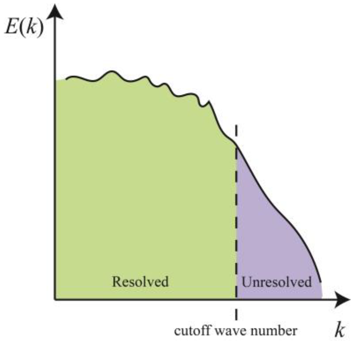
Figure 1. A stretch of the turbulence energy spectrum. The cutoff wave number separates the whole spectrum into resolved region and unresolved region. Resolved region can be captured by the available computation grid while the unresolved region cannot.
Fluids 10 00292 g001
Figure 2. Liutex spectrum as a function of wave number [21].
Fluids 10 00292 g002
Figure 3. A sketch of a cell with dimensions Δ x , Δ y and Δ z , and three Liutex components R x , R y and R z .
Fluids 10 00292 g003
Figure 4. Illustration of the computational domain. The bottom boundary is a flat plate.
Fluids 10 00292 g004
Figure 5. Vortex structures, represented by Liutex iso-surface R = 0.015 , for different models and grids: (a) DNS on G1, (b) no model on G2, (c) the proposed model on G2, and (d) WALE model on G2. In region A, only the proposed model on G2 successfully captures the first λ vortex. In region B, the proposed model clearly shows the formation of three vortex rings, while the vortex rings are not complete in no model and WALE model.
Fluids 10 00292 g005
Figure 6. Spanwise and time average of the velocity profile in wall units at x = 800 . The results of DNS on G1, no model on G2, WALE on G2 and the proposed model on G2 are depicted.
Fluids 10 00292 g006
Figure 7. Profiles of normalized and spanwise-averaged Reynolds stress components as functions of wall-normal coordinate z + for different approaches: (a) u + u + ¯ , (b) v + v + ¯ , (c) w + w + ¯ , (d) u + w + ¯ . Results are compared among DNS on G1 (cyan squares), no model on G2 (magenta diamonds), WALE on G2 (green circles), and the proposed model on G2 (black triangles).
Fluids 10 00292 g007
Figure 8. Comparison of time- and spanwise-averaged skin friction coefficient ( C f ) distributions along the streamwise direction ( x ) for different approaches. The DNS on G1 result is shown as a reference (cyan squares), while the WALE model on G2 (green circles), the no model case on G2 (magenta diamonds) and the proposed model on G2 (black triangles) are compared against DNS.
Fluids 10 00292 g008
Disclaimer/Publisher’s Note: The statements, opinions and data contained in all publications are solely those of the individual author(s) and contributor(s) and not of MDPI and/or the editor(s). MDPI and/or the editor(s) disclaim responsibility for any injury to people or property resulting from any ideas, methods, instructions or products referred to in the content.