Stabilization of Isolated Vortices in a Rotating Stratified Fluid

Abstract

The key element of Geophysical Fluid Dynamics—reorganization of potential vorticity (PV) by nonlinear processes—is studied numerically for isolated vortices in a uniform environment. Many theoretical studies and laboratory experiments suggest that axisymmetric vortices with a Gaussian shape are not able to remain circular owing to the growth of small perturbations in the typical parameter range of abundant long-lived vortices. An example of vortex destabilization and the eventual formation of more intense self-propagating structures is presented using a 3D rotating stratified Boussinesq numerical model. The peak vorticity growth found during the stages of strong elongation and fragmentation is related to the transfer of available potential energy into kinetic energy of vortices. In order to develop a theoretical model of a stable circular vortex with a small Burger number compatible with observations, we suggest a simple stabilizing procedure involving the modification of peripheral PV gradients. The results have important implications for better understanding of real-ocean eddies.

1. Introduction

Energetic jets and vortices dominate the kinetic energy of flows in planetary atmospheres and the oceans where they are known to play a crucial role in the fluid transport. Understanding their linear and nonlinear stability in a rotating stratified fluid was a subject of many studies in Geophysical Fluid Dynamics. The Gaussian model of pressure anomalies in the radial and vertical directions has been widely used for circular vortices in various theoretical studies as it fits oceanic and laboratory vortices reasonably well. However, such a model has been found to be unstable to small perturbations in the typical parameter range of observed long-lived vortices (see the discussion and references in [1]). The purpose of this work is to develop a smooth stable model of a three-dimensional (3D) axisymmetric vortex in a continuously stratified rotating fluid that can reflect longevity of real-ocean vortices.

The longevity of isolated vortices is closely related to their stability to small perturbations controlled mostly by the distribution of the potential vorticity (PV) along isopycnal surfaces. An isolated circular vortex with a small Rossby number is known to be stable if the radial gradient of PV does not change sign [2]. Typically ocean eddies are associated with pronounced PV anomalies (PVA) at the level of maximum azimuthal velocity. The vertical extent of the PVA cores is characterized by a maximum vertical displacement of isopycnal surfaces [3]. Baroclinic circular vortices with a constant PVA core, localized both radially and vertically, embedded in uniform PV exterior regions, represent the unconditionally stable states. Such structures have often been used by modelers to study the vortex interactions [4,5].

Generally, the presence of opposite PV gradients outside the vortex core does not necessarily imply the growth of perturbations: actual vortex instability depends on the details of the peripheral vortex structure and the ambient stratification. When the Burger number is small (i.e., the eddy is wide compared to the baroclinic radius of deformation) and has no flow at depth (compensated state), most of the theoretical studies with low vertical resolution (e.g., two-layer models) predict the growth of perturbations to an initially circular eddy owing to classical baroclinic instability unless the ocean depth is assumed to be unrealistically large (see [6] and references therein). The addition of a deep co-rotating circulation results in the stabilizing effect in circular eddies for a two-layer ocean model, which can be related to a reduction of opposite PV gradient in the lower layer [7,8,9]. Alternatively, the coupling between the upper and lower layers weakens if a third middle layer with uniform PV is added that also reduces the PV gradient in the deep layer at rest and enhances the stability of compensated vortices [1]. Here, we explore the more general idea of 3D vortex stabilization for a continuously stratified fluid by correcting peripheral PV gradients.

The nonlinear evolution of unstable circular vortices may result in the formation of various vortex structures including dipoles, tripoles, and multipoles as shown by numerical simulations and laboratory experiments. The possibility of monopolar eddies to transform into multipoles is well known both for two-dimensional (2D) and 3D stratified vortices. The book [5] and recent studies [10,11,12,13] describe various vortical structures and their transformations, and provide a comprehensive account of previous studies in this area.

Substantial progress in high-resolution observations and simulations has revealed an abundance of submesoscale and fine-scale structures in the oceans [14]. In particular, a clear evidence of the vertical stacking of sharp variations in density gradients (layering) at the periphery of deep ocean vortices, far from the upper ocean and the bottom, is provided by seismic imaging of the water column (see [15] and references therein). Whereas effects of double-diffusive convection were used for explaining the layering for years [16], recently it has been suggested that isopycnal stirring by the differential rotation in the vortex is able to generate the thin layers seen in seismic imaging [17]. On the other hand, stirring can be related to the baroclinic instability of localized eddies with substantial domain of opposite PV gradients below and/or above the vortex core [18,19].

In the present study, we demonstrate the nonlinear 3D evolution of an unstable circular Gaussian anticyclonic vortex in a continuously stratified rotating fluid resulting in vortex elongation and breaking into more intense self-propagating structures. In order to control vortex stability by a reduction of opposite PV gradients, we suggest an iterative method for balanced initialization of a stratified vortex based on prescribing PV along isopycnal surfaces. First, we look at the vortex fragmentation with PV distribution in Gaussian vortices used in previous studies. Second, we modify the initial vortex structure to eliminate opposite isopycnal PV gradients and confirm that such a vortex remains stable for decades in numerical model. Third, we show how the stable eddy can become weakly unstable depending on details of the model setup.

The manuscript is organized as follows. The 3D numerical model and results of simulations for a Gaussian vortex is described in Section 2. The structure of a circular vortex in isopycnal coordinates and an iteration scheme for prescribing the initial vortex for a given PV are presented Section 3. Section 4 presents the conclusions.

2. Instability of a Gaussian Vortex

To illustrate evolutionary features of vortices related to the details of its radial PV gradient, we present the numerical simulation of an intra-thermocline anticyclonic vortex (meddy) with a Gaussian shape of the angular rotation rate:

$$\mathsf{\Omega }\left(r,z\right)=-Rof\text{exp}\left(-\frac{r^2}{r_0^2}-\frac{{(z-z_0)}^2}{h^2}\right), P\left(r,z\right)=-\frac{r_0^2}{2}f\mathsf{\Omega }\left(r,z\right)\left[1-\frac{Ro}{2}\text{exp}\left(-\frac{r^2}{r_0^2}\right)\right].$$

(1)

Here, Ro is the Rossby number, f is the Coriolis parameter, $r_0$ is the vortex radius, h is the vertical scale, r is the horizontal distance from the vortex center, z is the vertical coordinate, and $z_0$ is the level of maximum azimuthal velocity $v=r\mathsf{\Omega }$. The pressure anomaly ${\rho }_{0}P$ (${\rho }_0$ is the reference density) is prescribed from the cyclo-geostrophic balance:

$$\mathsf{\Omega }\left(f+\mathsf{\Omega }\right)=\frac{\partial P}{r\partial r}.$$

(2)

The corresponding density field ρ is obtained from the hydrostatic balance

$$\frac{g\rho }{{\rho }_0}+N_0^{2}z=-\frac{\partial P}{\partial z},$$

(3)

where $N_0$ is the background buoyancy frequency that gives the minimum value of buoyancy frequency $N_c$ at the vortex center and the Burger number Bu

$$\frac{N_c^2}{N_0^2}=1-\frac{Ro}{Bu}\left(1-\frac{Ro}{2}\right), Bu= \frac{N_0^2{h}^2}{f^2{r}_0^2}.$$

(4)

The Ertel PV in such circular vortex can be written as

$$PV=\frac{N^2}{N_0^2}\left(f+2\mathsf{\Omega }+r{\left\{\frac{\partial \mathsf{\Omega }}{\partial r}\right\}}_{\xi =const}\right),$$

(5)

where the radial gradient of $\mathsf{\Omega }$ is calculated along isopycnals described by the coordinate ξ (see the next section). The PV anomaly ($PVA=PV-f$) is also used further to characterize the vortex structure.

In the following numerical simulation, $f={10}^{-4}\hspace{0.17em}{\mathrm{s}}^{-1}$, $r_0=30\hspace{0.17em}\mathrm{km}$, $h=400\hspace{0.17em}\mathrm{m}$ and the meddy is embedded in a uniformly stratified ocean with buoyancy frequency of $N_0=2.8\times {10}^{-3}\hspace{0.17em}{\mathrm{s}}^{-1}$, so that $Bu=0.14$ while $Ro=0.1$. For this value of Bu, the growth rate of the fastest growing azimuthal mode (m = 2) in the quasigeostrophic approximation ($Ro\ll 1$) is about 0.0007 f, according to [18].

The numerical model used in this study is the Massachusetts Institute of Technology (MIT) general circulation model [20,21]. The computational domain of 480 km × 480 km × 2 km is resolved by the uniform mesh with 256 × 256 × 200 grid points in x, y, and z, respectively. Periodic boundary conditions were assumed in x and y, and the free-slip boundary condition was applied at the bottom. The model was integrated in time with the time-step of $\Delta t=100$ s.

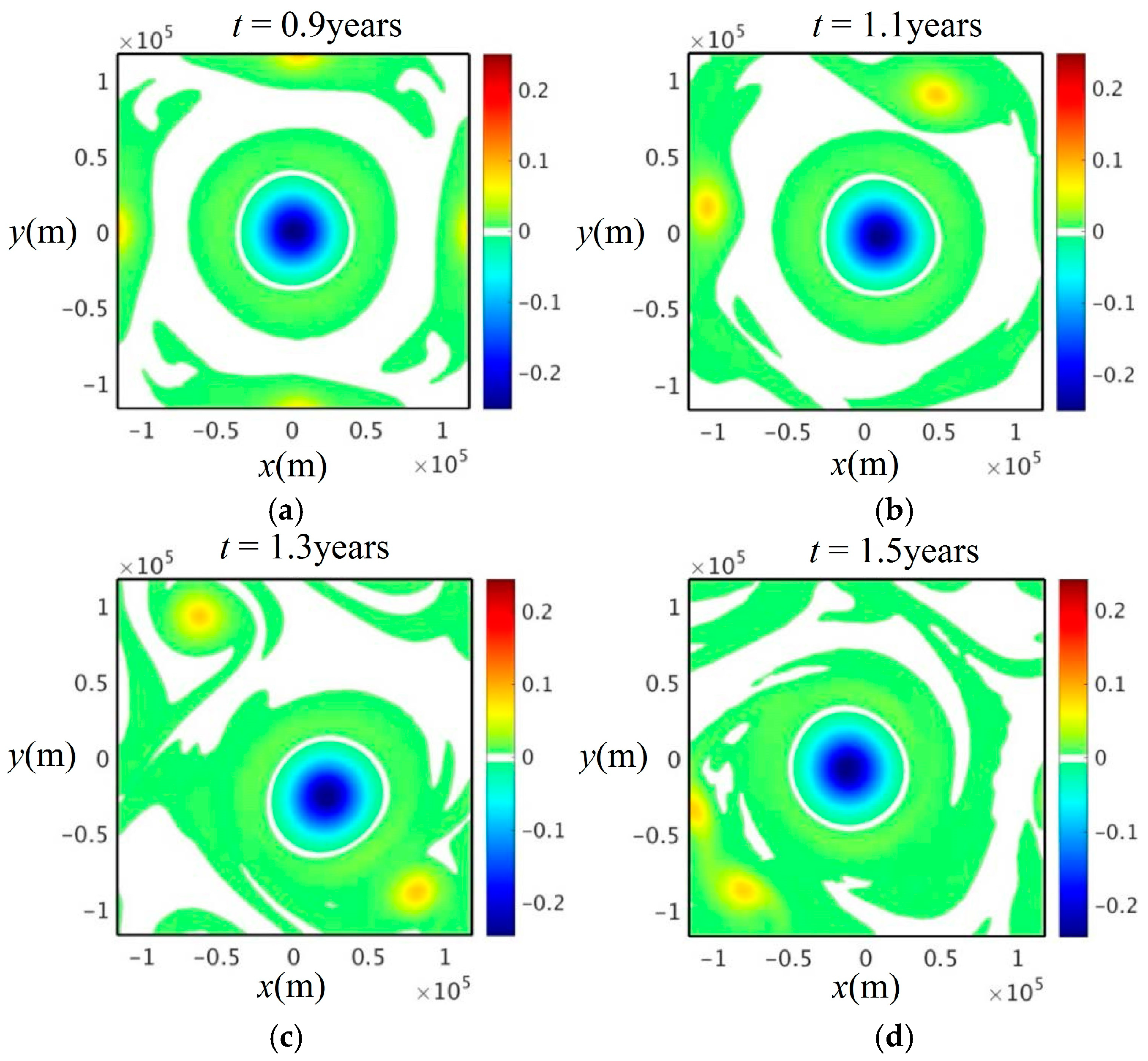
Radial profiles of initial PV (Equation (5)) interpolated into isopycnal surfaces display domains of opposite PV gradients above and below the major vortex core (Figure 1a). The axisymmetric state is an exact steady solution of the model, and the development of small perturbations results from rounding errors in the numerical code. After 300 days of integration, the instability of the Gaussian meddy results in the elongation of the main vortex core of negative vorticity and the splitting of the outer annulus of positive vorticity into two satellites with outward spirals (Figure 2a). Two months later, the elongated core broke into two pieces (Figure 2b), which propagated in opposite directions (Figure 2c,d). This scenario of severe elongation and fragmentation of the vortex core is typical for strongly unstable vortices with dominant azimuthal mode m = 2 in the two-layer models, e.g., [5,8,11,13,22]. For continuously stratified fluid, this scenario was described in quasigeostrophic contour-dynamical model as heton instability for vertically offset negative and positive equal vortex cores with uniform PV [23]. Less severe instability of a Gaussian vortex may result in shedding smaller vortices with a substantial reduction of the interior circulation of a surviving vortex in 3D simulations [24].

A remarkable feature of the development of vortex instability is a dramatic growth of the peak vorticity and kinetic energy during the elongation stage and vortex fragmentation (Figure 3). To a lesser degree, the growth of peak vorticity in unstable cyclones was noticed 30 years ago in the two-layer model [22] and for elongating anticyclones in the three-layer model [13]. Clearly, it is related to the conversion from the potential energy of the initial vortex into kinetic energy that is typical for baroclinic instability (Figure 3b). Development of sharp vorticity gradients during the elongation stage can be seen around the vortex core in Figure 4a,c which are similar to Figure 5a,c in the three-layer model [13]. Figure 4b,d illustrate that vortices resulting from the core fragmentation are smaller but rotating more rapidly. Such a mechanism of vortex energizing deserves further investigation.

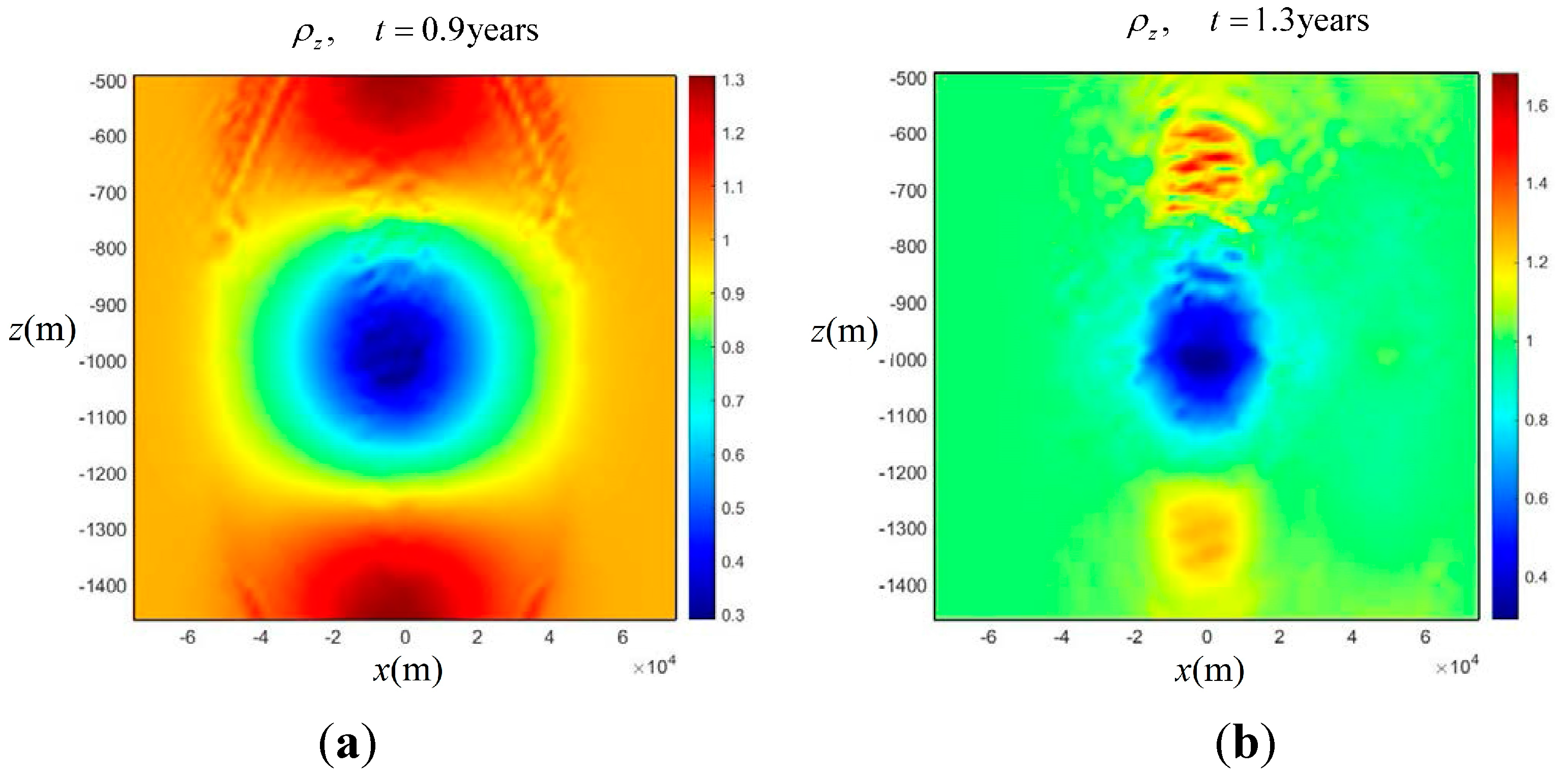
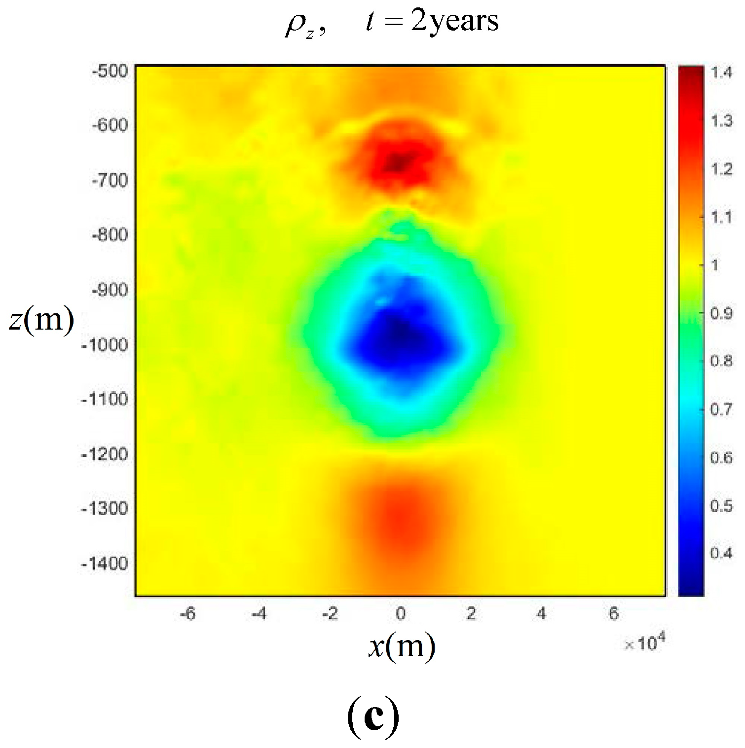
For small Bu, the major contribution to PV is related to the vortex stretching characterized by $N^2/N_0^2$ (the first term in (2.5)). The sign of the vortex stretching changes between the vortex core and upper/lower domains of opposite PVA. For an anticyclonic meddy, the isopycnals in the core are stretched, while in domains above and below the core, they are squeezed (Figure 5). Note that during the elongation stage, domains of vortex squeezing remain vertically aligned with the vortex core (Figure 5a). After fragmentation, formation of layering above smaller vortices is evident in Figure 5b, which is similar to the results presented in [19]. Apparently, it arises due to isopycnal stirring by the differential rotation in the vortex as suggested in [17]. Note that the vortex stretching is vertically symmetric in the quasigeostrophic model, while in the more accurate Boussinesq model, the upper domain display stronger layering similar to the observation in Figure 2 [19]. In this numerical model, the layering diffuses at the later stages while the smaller vortices do not display instability despite the presence of regions with opposite PVA (Figure 5c). Further studies are needed to clarify the stability properties of smaller self-propagating vortices with nearly double values of Ro and Bu.

3. Theoretical Model of a Stable Vortex

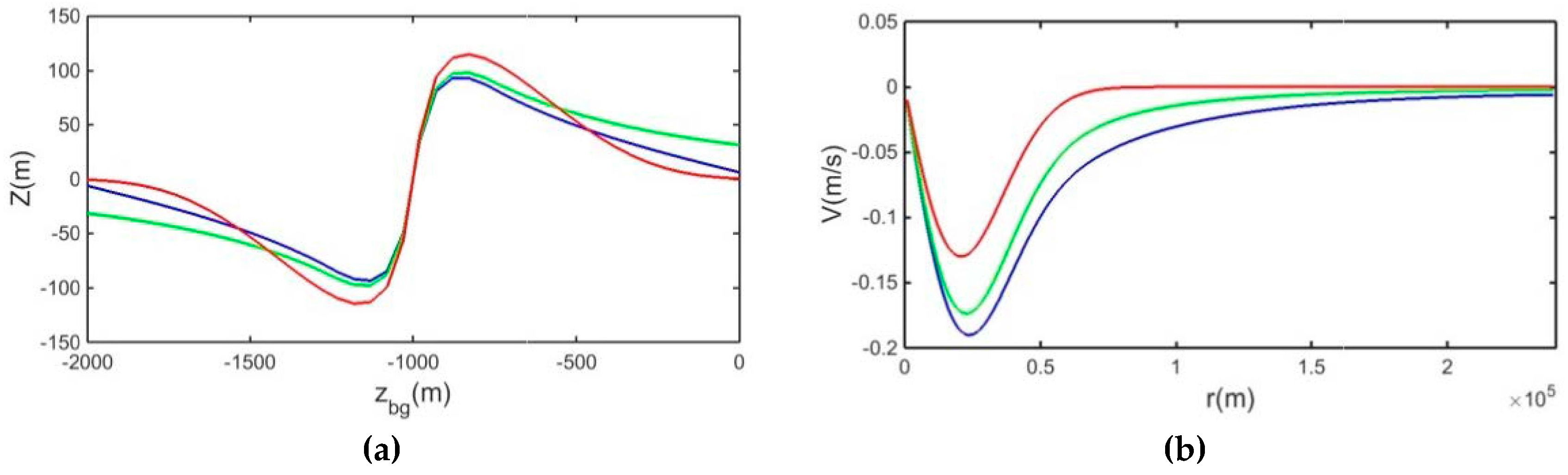
Consider an axisymmetric vortex in an f-plane, ocean model with constant total depth H using the cylindrical isopycnal coordinates (r, ξ), ξ is the unperturbed depth of isopycnal surfaces, which is further used instead of the vertical coordinate. Then, Z(r, ξ) can be introduced for the vertical displacement of isopycnal depths from their unperturbed levels. A typical profile of Z(0, ξ) at the vortex center is shown in Figure 6a (see also Figure 4 in [3]). Then, the Equations (2) and (3) can be transformed to the form:

$$\mathsf{\Omega }\left(f+\mathsf{\Omega }\right)=\frac{\partial \Pi }{r\partial r}, {\Pi }_0\left(\xi \right)=-{{\displaystyle \int }}_0^{\infty }\mathsf{\Omega }(f+\mathsf{\Omega })rdr,$$

(6)

$$-N_0^{2}Z= \frac{\partial \Pi }{\partial \xi }, -N_0^2\frac{\partial Z}{r\partial r}=\left(f+2\mathsf{\Omega }\right)\frac{\partial }{\partial \xi }\mathsf{\Omega },$$

(7)

where $\Pi =P+\rho gz/{\rho }_0+N_0^2{z}^2/2$ is the anomaly of the Montgomery potential. It has an extremum value ${\Pi }_0\left({\xi }_0\right)$ at some isopycnal level ${\xi }_0$ that remains horizontal, i.e., Z($r, {\xi }_0$) = 0. When ${\xi }_0$ is near the sea surface, such vortex is surface intensified (which is typical for the ocean rings), while for intrathermocline eddies ${\xi }_0$ can be at any depth. The vertical boundary of the vortex core with the main PVA is marked by the isopycnal surface corresponding to maximum Z at the vortex center in the same manner as the radial extent of PVA is marked by the maximum azimuthal velocity $r_c\mathsf{\Omega }$ ($r_c$, ${\xi }_0)$. Here,

$$\mathrm{PVA}=2\mathsf{\Omega }+r\frac{\partial \mathsf{\Omega }}{\partial r}-\mathrm{PV}\frac{\partial Z}{\partial \xi },$$

(8)

$$\frac{\partial }{r\partial r}\left(r^2\frac{\partial \mathsf{\Omega }}{\partial \xi }\right)-\frac{\partial }{\partial \xi }\left(\mathrm{PV}\frac{\partial Z}{\partial \xi }\right)=\frac{\partial \mathrm{PV}}{\partial \xi }.$$

(9)

The observed structure of ocean rings and intrathermocline eddies can be represented realistically by a vortex with uniform PVA inside the vortex core and zero PVA outside the vortex core [3]. In this case, the radial PV gradient does not change sign, which guarantees stability of such a vortex to small perturbations in balanced models. In order to determine the vortex structure for a given PV distribution, we combine Equations (7) and (9) to get an elliptic equation for Z:

$$\frac{\partial }{r\partial r}\left(\frac{r{N}_0^2}{f+2\mathsf{\Omega }}\frac{\partial Z}{\partial r}\right)+\frac{\partial }{\partial \xi }\left(\mathrm{PV}\frac{\partial Z}{\partial \xi }\right)=\frac{\partial \mathrm{PV}}{\partial \xi },$$

(10)

which is solved by an iterative method with boundary conditions Z = 0 at the middle level ${\xi }_0$ and far from the vortex core $r, \xi \to \infty$. Corresponding Π and Ω are calculated from Equations (6) and (7). In order to minimize the (potentially destabilizing) influence of the upper and lower boundaries on the eddy, we consider solutions in which isopycnals are horizontal at the sea surface and the bottom. This is accomplished by adding to the solution Equation (10) its mirror images with respect to the surface and to the bottom, i.e., symmetric structures centered at $-{\xi }_0$ and $2H-{\xi }_0$.

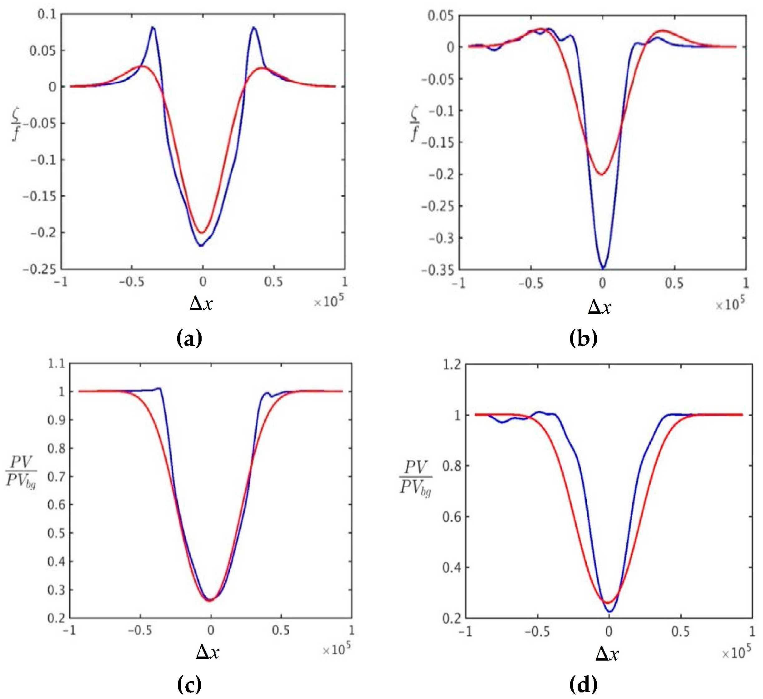
For a Gaussian vortex, the domains with opposite PVA are located below and above the major vortex core (Figure 1a) (see also Figure 2 in [17]), which provide a source of baroclinic instability described in Section 2. This PV pattern was interpolated into isopycnal coordinates and the regions with negative radial PV gradients were effectively eliminated by replacing them with the uniform PV zones (Figure 1b). The resulting solution to Equation (10) has been re-interpolated into the Cartesian coordinate system, and its evolution was simulated using 3D model described in Section 2. While PV-corrected isopycnal displacement does not differ much from that in the Gaussian vortex (Figure 6a), the azimuthal velocity is substantially increased in the PV-corrected case (Figure 6b). Such a solution with uniform PV outside the vortex core corresponds to the two-layer corotating state considered by Benilov [9]. Note that without adding mirror images, the isopycnal displacement remains substantial near the surface and the bottom (Figure 6a), leading to radial density gradients near the surface and the bottom, which may also induce Eady-type baroclinic instability.

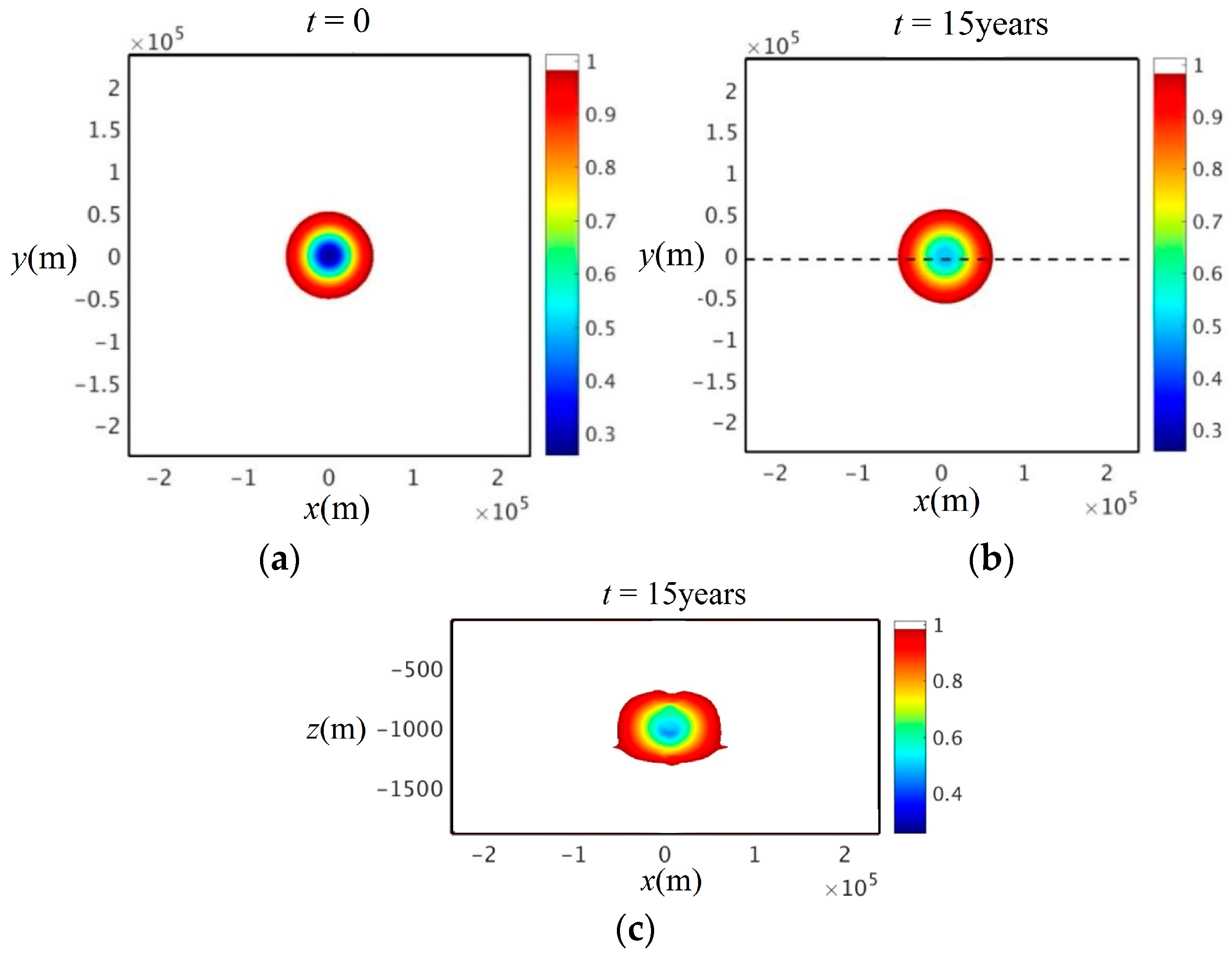
Figure 7 illustrates that PV-corrected state remains axisymmetric in the numerical simulations for many years. Note that for a smaller computational domain (Figure 8) or without mirror image adjustment (Figure 9), the numerical solutions display weak instability.

4. Conclusions

We have demonstrated that a Gaussian model for 3D axisymmetric vortex with small Bu in a rotating stratified fluid displays strong instability manifested by the growth of the second azimuthal mode corresponding to the quasigeostrophic linear analysis [18]. Further nonlinear elongation and fragmentation of the vortex core into pieces are consistent with previous studies using layered models, e.g., [8,13,20] as well as with 3D quasigeostrophic contour dynamical simulations [21]. The peak vorticity growth found during the stages of strong elongation and fragmentation is related to the transfer of available potential energy into kinetic energy and may play an important role in the longevity of ocean vortices.

In order to design a theoretical model of stable oceanic vortices, an iterative procedure was implemented, which eliminated the opposite radial isopycnal PV gradients. Corresponding isopycnal displacement in the PV-corrected vortex does not differ significantly from the original Gaussian model, while the azimuthal velocity is substantially stronger. Such a modified vortex is shown to remain axisymmetric and stable for a number of years in the numerical model, although there is no a theoretical justification that the absence of an opposite PV gradient is a sufficient condition for stability in a non-hydrostatic, finite Rossby number case [25]. It was shown that for a smaller computational domain or without mirror image adjustment, the numerical solutions display weak instability. The proposed technique for development of stable realistic vortex models by controlling opposite PV gradients can be profitably employed in further investigations of the dynamics and structure of oceanic eddies.