Article

A Comparative Analysis of Machine Learning Models for the Prediction of Insurance Uptake in Kenya

by
Nelson Kemboi Yego
1,2,*,
Juma Kasozi
1,3 and
Joseph Nkurunziza
1,4
1
African Center of Excellence in Data Science, University of Rwanda, Kigali, Rwanda
2
Faculty of Sciences, Department of Mathematics and Computing, Moi University, Eldoret 3900-30100, Kenya
3
Faculty of Physical Sciences, Department of Mathematics, Makerere University, Kampala 7062-10218, Uganda
4
School of Economics, University of Rwanda, Kigali, Rwanda
*
Author to whom correspondence should be addressed.
Data 2021, 6(11), 116; https://doi.org/10.3390/data6110116
Submission received: 28 January 2021 / Revised: 8 March 2021 / Accepted: 10 March 2021 / Published: 15 November 2021
(This article belongs to the Special Issue Data Analysis for Financial Markets)

Abstract

:
The role of insurance in financial inclusion and economic growth, in general, is immense and is increasingly being recognized. However, low uptake impedes the growth of the sector, hence the need for a model that robustly predicts insurance uptake among potential clients. This study undertook a two phase comparison of machine learning classifiers. Phase I had eight machine learning models compared for their performance in predicting the insurance uptake using 2016 Kenya FinAccessHousehold Survey data. Taking Phase I as a base in Phase II, random forest and XGBoost were compared with four deep learning classifiers using 2019 Kenya FinAccess Household Survey data. The random forest model trained on oversampled data showed the highest F1-score, accuracy, and precision. The area under the receiver operating characteristic curve was furthermore highest for random forest; hence, it could be construed as the most robust model for predicting the insurance uptake. Finally, the most important features in predicting insurance uptake as extracted from the random forest model were income, bank usage, and ability and willingness to support others. Hence, there is a need for a design and distribution of low income based products, and bancassurance could be said to be a plausible channel for the distribution of insurance products.

1. Introduction

The role of insurance in financial inclusion, as well as in sustainable economic growth is immense and has been increasingly recognized. Insurance is not only important for its risk pooling and transfer roles, but also for capital accumulation for investment. Nevertheless, less discussion has been done about its importance. Much of the discussion has been on the banking sector, but less on the insurance sector [1,2]. Olayungbo and Akinlo [1] recommended financial reforms and called for wide insurance coverage for insurance development. The wide range coverage could be achieved with the targeted distribution of insurance products, which results in higher uptake. Since the African Union Agenda 2063 envisions inclusive sustainable development in Africa, insurance could contribute a great deal to achieving this. This is more so due to the tendency of financial risks to increase over time. Therefore, the sustainability of the growth could be cushioned by hedging the risks, and in this, insurers are better placed for their ability to indemnify their clients in case of a peril operation [3,4].
Despite its role in financial inclusion and sustainable economic growth, low insurance uptake and low penetration have seemed to impede the growth of the insurance sector. Insurance uptake has been low in Kenya. This has been regardless of various programs developed and implemented by the Association of Kenya Insurers (AKI) to increase the uptake and consequently the penetration. Moreover, life insurance penetration in the Kenyan market had worsened for the third year in a row, dipping to 2.79 % in 2015 from 2.94 % in 2014. This was even though the gross domestic product (GDP) grew to 5.6 % in 2015 in comparison to 5.3 % in 2014. The low uptake has spanned most lines of insurance. Uptake of insurance has been one of the impediments to the growth and expansion of insurance. This is possible because low uptake directly affects financial performance since the lower the uptake, the lower the penetration and, consequently, the lower the financial performance [5].
The paper begins with the Introduction, where the motivating problem and the objectives of the study are brought up. It then moves to related literature where works relating to insurance uptake, as well as those relating to the machine learning used are reviewed. In the Methodology Section, we describe the data used and the analysis done to arrive at the results. The Results and Discussion Section discusses the findings in both Phase I and Phase II of the analysis. We finally make some conclusions and recommendations based on the findings.

2. Related Literature

2.1. Insurance Uptake

Uptake could be investigated from the demand side of insurance in terms of the count of people who take up policies, while penetration could be thought of as premiums as a ratio of gross domestic product. Nevertheless, both ways of looking at insurance growth have shown low statistics. The problem of low insurance uptake could be alleviated by targeted uptake promotion, hence the need for a model that robustly predicts uptake. Finding an optimal and robust way of predicting insurance policy uptake can help determine whether a customer or a potential one will take up insurance. Such a model would be valuable from the insurers’ point of view, especially in putting in place a distribution strategy for insurance. This will help in targeted marketing and product improvement [6].
Previous studies related to this paper focused on a particular line of insurance, and none made use of the machine learning approach, for instance the uptake of private health insurance, community based kinds of health insurance, remote sensing insurance, flood insurance, and agricultural insurance. Whereas these are vital in ensuring in-depth knowledge of these particular lines, there is a need to have a look at the overall picture of insurance as a whole Lambregts and Schut [4]. This study attempts to fill this gap by having a look into the insurance uptake prediction from an overall perspective by considering all the lines of insurance. The labels are therefore related to insurance uptake on all the lines: life, non-life, and health insurance.

2.2. Use of Machine Learning Models

The use of machine learning is motivated by its predictive capabilities and the documented possibility of yielding new insights. Moreover, machine learning takes advantage of the available data to glean insights and make the predictions, hence the possibility of new insights hitherto unforeseen [7]. It has been found that combined use of machine learning and data, in particular large data, allows for greater analysis and coming up with better models that would not be possible with traditional methods [8,9]. Grize et al. [9] emphasized that the application of machine learning in insurance is bound to increase in the foreseeable future. The target variable had a binary label; hence, the supervised learning problem was classification in nature. Therefore, this paper attempts to address a classification problem that compares machine learning models that classify an insurance potential client as either taking up a policy or otherwise based on features of the potential customer, mostly socio-demographic in nature.
Whereas machine learning may not have been applied in insurance uptake prediction, it has had applications in other areas of business and insurance ranging from the application to modeling of life insurance companies [10], as well as in export credit finance claims prediction [11], the cost-sensitive type of credit scoring [12], time series related data including stock prices [13,14], and even in product sentiment analysis [15]. Recommender algorithms have also been used in making recommendations to insurance clients on policies, as well as in purchase prediction [2]. Both supervised and unsupervised techniques have been applied in business areas. Clustering has had many applications in unsupervised areas, while the supervised area has mostly focused on prediction or forecasting [16,17]. Grize et al. [9] further asserted that machine learning applications in insurance have had an increasing relevance. Machine learning and data mining methods including clustering, classification, and regression methods, in particular classification and regression trees, ensemble methods (like random forests, extreme gradient boosting), support vector machines, neural networks, and deep learning methods have all had applications in insurance.
From the previous works that applied machine learning in insurance, Zhou et al. [2] contributed to feature selection by proposing a multi-label entropy based feature method of selecting features in insurance purchase prediction. They found that clients look for personalized products suitable for their particular financial situation, family financial background, and individual risk tolerance. This implies that the use of personal and household social and demographic features as used in the current paper is warranted. Grize et al. [9] made the assertion that machine learning applications in insurance are bound to increase. They put forward that risk assessment capacity is improved and the speed of developing better models is higher with machine learning. They further put forward that new products, processes, and even new insurers are bound to arise from the opportunities offered by digitization, AI, and machine learning. In this, they stressed the importance of data and their quality as an important ingredient in machine learning modeling. This study sought to find a robust way of assessing the uptake of clients using machine learning based on the recent data.
Each of the models considered in this study has had previous optimal performance in other studies, hence their inclusion for comparison in this study. For instance, random forest, support vector machine, and decision trees have been found to perform with high sensitivity each, in insurance-related data [18]. A classifier can be defined as: for a sequence set of label Y and sequence domain set X , we sought an optimal classifier h that predicts a new customer as taking up insurance or not such that the loss L s ( h ) in the test set is minimized. h : X Y , where H is the hypothesis class in which h is expected to fall [19].
h S argmin h H L S ( h )

2.2.1. Logistic Regression Classifier

The logistic regression classifier is derived from linear regression, but modified by a logistic function. For the outcome Y, which is the uptake of insurance or non-uptake for the current study, the outcome maybe one or zero otherwise.
Y = 1 , = uptake 0 , = non - uptake
for X = x 1 + + x n , where x 1 + + x n are the features under consideration. The probability that a customer or potential customer will take up insurance is given by [19]:
π ( x ) = E ( Y | x 1 x n ) = e x p { β 0 + β 1 x 1 + . . . + β n } 1 + e x p { β 0 + β 1 x 1 + . . . + β n }

2.2.2. Support Vector Machines

Support vector machines (SVMs) are a frontier hyperplane that optimally segregates two classes by seeking the largest margin between the nearest points of the training set of any class (referred to as support vectors). With the kernel trick, finite-dimensional space features could be mapped into a higher dimensional space, hence making it possible to linearly separate them despite the dimensional space [19]. SVM has been applied in diverse areas and has been found to have high accuracy in many instances including cancer diagnosis [20]. In this paper, the support vectors gave the largest margin between the insurance clients (and potential ones) who would uptake coverage and those who would not uptake, based on the features. In the case of Sundarkumar and Ravi [18], DT and SVM had high sensitivity in the insurance dataset compared to logistic regression, MLP, and the probabilistic neural network.

2.2.3. Gaussian Naive Bayes)

Gaussian naive Bayes (GNB) determines the posterior probability of taking up insurance given the features. Given the value of the label, y, the algorithm takes Bayes’ theorem, but with the assumption of conditional independence between every pair of covariates.
P ( y x 1 , , x n ) = P ( y ) P ( x 1 , x n y ) P ( x 1 , , x n )
y is the class label, and x 1 , , x n are the features. The class label in this research is the uptake, while the covariates are the features used. The classifier, therefore, works by comparing the posterior distribution of each of the two classes (which may either be uptake or non-uptake) and takes the higher.

2.2.4. K Nearest Neighbor

The classifier in KNN is such that for a training set S and for every point x i n X , it outputs the highest of the labels among ( y π i ( x ) : 1 k ) , where π 1 ( x . . π m ( x ) is the reordered set S , ordered as per their distance to x . The distance, in this case, is the Euclidean distance. The classifier finds the Euclidean distance between new data points for each training example. It then selects the K entries closest to the new data point. The label with the highest frequency in K entries will be the class label of the new data point. Therefore, if the most common is non-uptake, the new data point will be classified as non-uptake and vice versa [19].

2.2.5. Decision Trees

These are classifiers, h : X Y , that predict the label associated with an instance of, say variables, by moving from the root node to a leaf. DT is built as branch-like fragments. The decision tree consists of root nodes and leaf nodes signifying the class labels, whereas the intermediate nodes denote non-leaf nodes. The data attribute with the highest priority in decision-making is selected as the root node. The splitting process of a decision tree is decided upon by the data values of the respective nodes. The decision tree learns during the training phase, and its effectiveness is evaluated during the testing phase. The depth and the distribution of the training and test information of DT dynamically impact the performance and efficiency of the classifier [21]. In this research, DT is applied to predict insurance uptake; leaf nodes represent classification labels, which may be either uptake or non-uptake. The inclusion of DT in this study was motivated by the need to compare it with its respective ensemble algorithms: random forest and gradient boosting. Moreover, DT as a model has had applications ranging from health [22] to network anomaly detection [23].

2.2.6. Random Forest

Random forest is a tree based algorithm whose trees are assembled by bagging. The trees are independently trained. The random forest classifier uses an ensemble of decision trees to predict insurance uptake based on features. The prediction is the outcome of sequential, binary decisions that are orthogonal split in the multivariate space of variables. In this case, therefore, the random forest classifier is taken as the classifying algorithm, that is a meta learner of several trees built independently of each other. Random forest has compared favorably with other ensemble decision tree based models in previous studies. In some cases, it performs better than other learners [24], but in others like the case of [25], boosting performed better.

2.2.7. Gradient Boosting Machine and Extreme Gradient Boosting

Gradient boosting machines (GBMs) and extreme gradient boosting (XGB) are tree based supervised learning models. Their ensemble method of learning is by boosting. The classification trees are sequentially trained to improve the performance of the next tree from the previous one. As a result, every new tree attempts to correct the errors of the preceding tree. GBM and XGB only differ from the point that XGB uses a more formalized regularization than GBM. This makes controlling for overfitting better and gives better model performance. Gradient boosting methods have been found to perform well, yielding state-of-the-art results in most classification and regression tasks compared to other models [25].

2.2.8. Deep Learning Classifiers

There has been growing interest in deep learning models because they have been found to outperform the traditional classifiers. In this study, deep learning classifiers are used on the FinAcss2019 data and compared with the two tree based classifiers. The multilayer perceptron (MLP), convolutional neural networks (CNNs), and long short-term memory (LSTM) deep learning classifiers are considered. Deep CNNs have previously been found to demonstrate better performance compared to over state-of-the-art MLPs [15]. Dashtipour et al. [15] furthermore recommended the use of LSTM. Moreover, a CNN-LSTM model has been used recently in prediction and found to improve the performance as compared to a normal LSTM model [26]. Besides, the CNN-LSTM model in Sun et al. [27] outperformed the pure CNN or LSTM models on soybean crop yield prediction.
This study adds to the literature by bringing the machine learning model that robustly predicts insurance uptake upon comparing with several models. It also compares the performances of the machine learning models on both oversampled and downsampled data. It further gives the features that are important in insurance uptake prediction as extracted from the most robust model.

3. Methodology

The study has two phases. Phase I involved the comparison of 8 classifiers for insurance uptake prediction with 2016 Kenya FinAccess household survey data, while Phase II involved using Phase I as the base, in which the two most robust models from Phase I were included in Phase II and compared with 4 deep learning classifiers. In Phase I, recent 2019 Kenya FinAccess household survey data were utilized in the training and testing of the classifiers.

3.1. Data

The study used 2016 and 2019 Kenya FinAccess household survey data. Among the main objectives of the survey was to measure access to and demand for financial services among adults. The sample of the survey was representative of the whole country and based on the KNBSNASSEPVnational household sampling frame. The survey undertook 10,008 interviews from 834 clusters across the country, with 14 households being targeted in each cluster. A KISH grid was then used to select respondents at the household level. The sample drawn was representative downwards to 13 subregions in the country, which were clusters. These were: North Rift region, Central Rift region, South Rift region, Nyanza region, Western region, Eastern region, Coastal region, North Eastern region, Nairobi, and Mombasa. The survey was intended to measure access to and demand for financial services among Kenyans aged 16 years and above. A nationally representative cross-sectional survey used a multi-stage stratified cluster sampling design. About 834 clusters were initially selected as primary sampling units (PSUs), using the probability proportional to size (PPS), from a national sampling frame. The Fifth National Sample Survey and Evaluation Program (NASSEPV) was designed by the Kenya National Bureau of Statistics, according to Kenya’s previous population census (2009 population census). Furthermore, there was stratification according to urban and rural areas together with the country’s 47 counties, hence resulting in 92 strata. The second stage involved selecting 14 households in each cluster. In the final stage, one individual aged 16 years old and above was randomly selected per household using the KISH grid. There were 8665 interviews in 820 clusters conducted. One person was interviewed per household. Data were collected on socio-demographic characteristics, access, and use of financial services including mobile money and social health insurance enrollment [28].

3.2. Preprocessing and Features’ Selection

The aim of the supervised learning adopted in this paper was to find a learner that classifies an insurance customer or a potential one optimally and robustly. The 2016 Kenya FinAccess household survey data contained many variables, but only 30 relevant socio-demographic features were selected. Those that were highly co-varied and those with the least correlation were picked. This reduced the dimensionality, hence reducing the likelihood of overfitting. From the 30 features, eighteen features were selected based on a univariate selection where features with the strongest relationship with the label were taken. The univariate selection compared each feature with the label to check if there was a significant relationship. This feature selection method mechanism is such that it selects the best features based on univariate statistical tests. It compared each feature to the label variable, which was uptake in the case of this research, to check whether there was any statistically significant relationship between them. When comparing the relationship between one feature and the target variable, we ignored the other features. Each feature, therefore, had a test score. Lastly, the test scores from each feature were compared, and the features with the top scores were selected. This method was chosen for its flexibility for the given kind of data. All 18 features used in the final analysis had no missing values.
Similarly, the 2019 Kenya FinAccess household survey data had many variables each with 8669 observations, but only 35 were included in the study. The data had 4279 missing cells, which were 1.40% of the data. One of the variables had 2131 missing cells, which accounted for 24.6% of its observations, while another had 2148 missing values, which accounted for 24.8% its observations. The missing data were therefore observed in the two variables, and as a result, the two features were excluded from the final analysis. From the 35 features, twenty-five features were selected based on univariate selection. All the features in the 2016 Kenya FinAccess household survey data were included in the 2019 Kenya FinAccess household survey data with some seven additional features. The label set was uptake, while the instances in the domain set considered included vector features: gender, marital status, age group, education, numeracy, place of residence, Internet access, own phone, electricity as the main light source, smartphone, youth, wealth quintile, having a bank product, top trusted provider, second top trusted provider, residence, household size, having some fund set aside for an emergency, and the subregion in which one resided in the country. One hot encoding was performed on the categorical features to enable better prediction as factors. Uptake in this study implies the uptake of insurance regardless of the line or class of insurance. Those included in this label were those who had any kind of insurance coverage, whether life, non-life, or medical.

3.3. Handling Class Imbalance

The class imbalance problem arises when the data have a proportion of one class (majority class) significantly higher in than another (minority class). This could be alleviated by various techniques including oversampling of the minority class or undersampling of the majority class to balance both classes [29]. The Kenya FinAccess Household survey data used in the study, as is commonly the case in real-world settings, were imbalanced to an extent proportionally. Figure 1 shows the data balance proportion for the 2016 Kenya FinAccess Household survey data used. The proportion of those who did not have insurance to those who had it was 6807:1858, which is 3.66:1; hence, the data were unbalanced with the minority class being 21% of the data, while the majority class was 79%. Figure 1 demonstrates the class to some level of imbalance between uptake (the minority class) and non-uptake (the majority class). When the event of interest underrepresented uptake (the minority class), there was a tendency to hinder the classification accuracy. Data imbalance was handled by both upsampling and downsampling.
Figure 2 shows the data balance proportion for the 2019 Kenya FinAccess Household survey data used in the Phase II analysis. The proportion of those who did not have insurance to those who had it was 6139:2530; hence, the data were unbalanced with the minority class being 29% of the data, while the majority class was 71%. Despite the imbalance, there was a reduction in the level of imbalance between 2016 and 2019, implying there was an improvement in the level of uptake between the periods.

3.4. Model Performance Measures

Precision scores refer to the number of true positives divided by all positive predictions. The value is a measure of a classifier’s exactness. Low precision indicates a high number of false positives. The recall score refers to the number of true positives divided by the number of positive values in the test data. Low recall indicates a high number of false negatives. Sensitivity or the true positive rate is a measure of a classifier’s completeness. The F1-score is the weighted average of precision and recall.
A confusion matrix is a table showing correct predictions and types of incorrect predictions. True positives ( T P ) refer to the number of cases correctly identified as having taken insurance False positives ( F P ) are the number of cases incorrectly identified as having taken insurance True negatives ( T N ) are the number of cases correctly identified as not having insurance False negatives ( F N ) are the number of cases incorrectly identified as not having insurance.
A c c u r a c y = ( T P + T N ) ( T P + T N + F P + F N )
S e n s i t i v i t y = T P ( T P + F N )
S p e c i f i c i t y = T N ( T N + F P )

3.5. Hyperparameter Optimization

Grid searches were conducted to find hyperparameters that would yield optimal model performance. A 5-fold cross-validation technique was used based on accuracy as an evaluation metric.
Table A1 shows the hyperparameters tuned in RF. The hyperparameters for random forest that were tuned were: n_estimators, max_features, min_samples _split, and bootstrap. The n_estimators, which represent the number of trees in the forest, were optimized between 80 and 150 with a range of 10. Usually, the higher the n_estimators, the better the accuracy is, but upon optimizing, an optimum of 110 was found. The max_features are the maximum number of features that the model considers when splitting a node. The search was among auto, sqrt, and log2. The grid search for max_features was optimized as auto. The min_samples _split represents the minimum number of data points, from the total, that should be placed in a node before the node is split. The search was between 2, 4, 6, and 8, and it was optimized at 2. Finally, bootstrap represents the method used by the model to sample the data points, whether with a replacement or without. In this case, it is optimized at true, implying replacement.
Table A2 shows the hyperparameters tuned in the GBM. For the GBM, n_estimators were tuned among 100, 200, and 300 and optimized at 200. The parameter learning_rate was to control the weighting of new trees added to the model. The parameter was tuned between 0.01, 0.02, 0.05, and 0.1. The optimal learning_rate was found to be 0.05.
Table A3 shows the hyperparameter tuning on XGB. The parameters that were optimized were: n_estimators, max_depth, max_features, and gamma. For n_estimators, they were tuned between 500 and 1500, and the optimal was found at 1000. For max_depth, it was tuned among auto, sqrt, and log2, and the optimal arrived at was auto. On the other hand, max_features were tuned between 0.2 and 1, and the optimal arrived at was 0.9. Finally, gamma was tuned to 0.1.
The architectures of deep learning nets that were used were MLP, CNN, LSTM, and CNN-LSTM. The models designed with hyperparameters such as batch size, epochs, optimizer with learning rate, and dropout were tuned extensively to obtain optimized performance. The nets were trained from scratch, and the coefficients of the layers were randomly initialized. The training was performed for 300 epochs for the data. Whereas a smaller learning rate has been found not to converge to a suboptimal point, training tends to be slow, which may result in higher training error. It has further been observed that more training epochs could improve the performance for smaller learning rates. Hence, the learning rate of 0.001 was taken as a suitable rate to achieve moderate oscillations.

4. Results and Discussion

Python Version 3.6.1 was used as a tool for analysis. Python was used because it is malleable. Moreover, the various libraries that Python has made the analysis easier. A Jupyter notebook was the environment of choice for its simple interface. The results shown are for the test sample in each case. After data cleaning and the selection of relevant features, the data were split into three sets: training, validation, and test sets in the ratio of 0.75:0.15:0.10. For the training set, seventy-five percent of the data were used to train the algorithms. For the validation set, fifteen percent of the data were held back from the training of the model and were used to give an unbiased measure of model efficiency. The validation set was used to evaluate performance on data that were unseen when test data were held back. For the test set, ten percent of the data were held back from the training of the model and were used to give an unbiased measure of final model efficiency. The test set was held back until fine-tuning of the model was complete, and thereafter, an unbiased evaluation of the final models was obtained. Whereas Dashtipour et al. [15] used 60% as the data for training, 30% in testing, and 10% for validation, Pawluszek-Filipiak and Borkowski [30] observed that the performance metrics of the models, the F1-score and overall accuracy, decreased as the train-test ratio decreased. This implies that as the training sample decreases, the performance metrics tend to decrease. In line with the models’ need for substantial data to train on, Poria et al. [31] used 80% of the data for training, and the remaining 20% was partitioned equally between validation and testing. As a result, there was a need to choose a train-validation-test split ratio that not only optimized the accuracy, but also adequately measured the extent to which the model would perform on “unseen” data. These considerations informed the choice of the train-validation-test split ratio that was used.

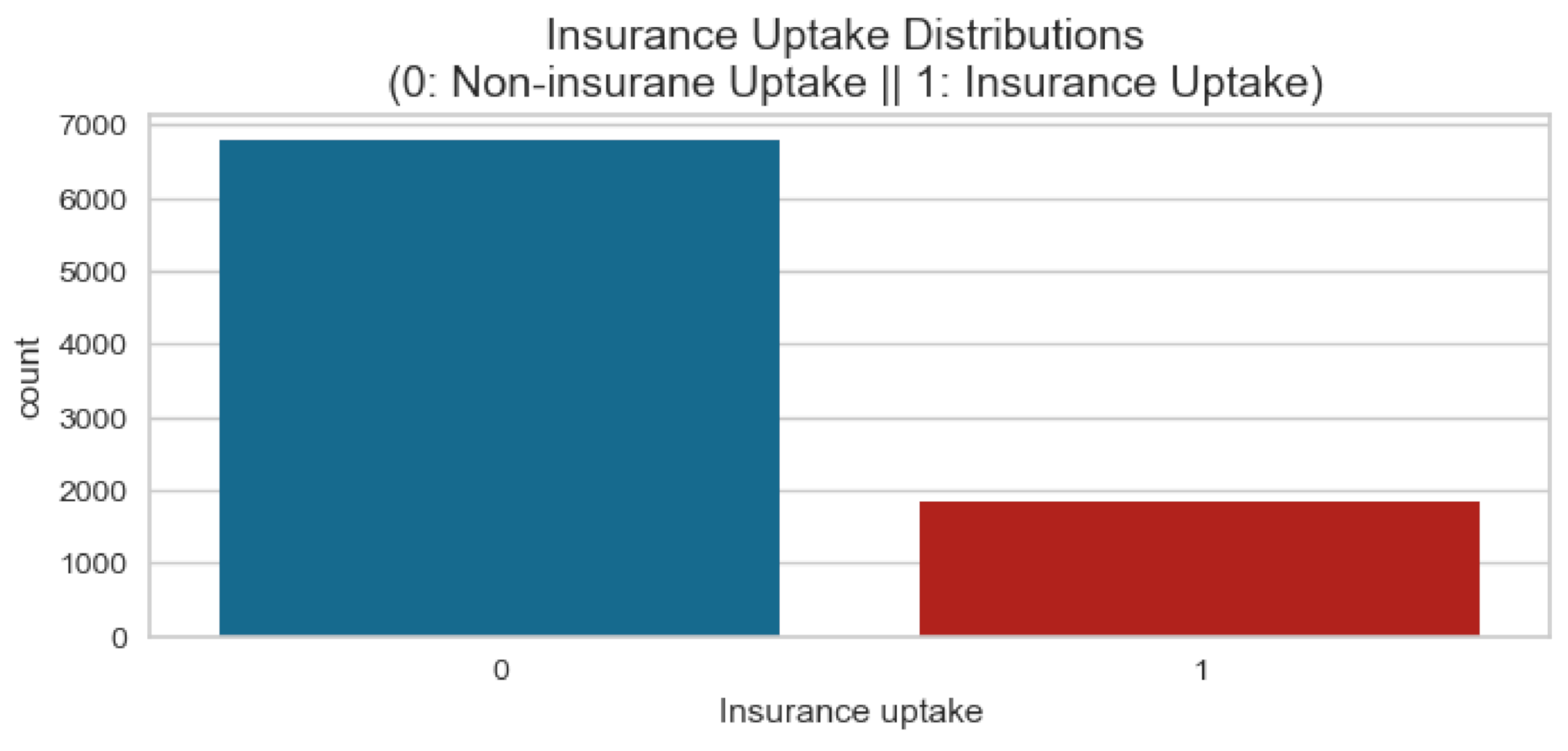
4.1. Comparison on Unbalanced Data

Table 1 shows the machine learning models and their respective precision scores, recall scores, F1-scores, and accuracy on the real unbalanced data. The XGB, SVM, GBM, and logistic regression classifiers had the highest accuracy (0.85) followed by random forest (0.82), KNN (0.81), and GNB (0.76), and the lowest was DT (0.75). For F1-scores, logistic regression showed the highest (0.61), then XGB (0.60), GBM (0.59), SVM (0.58), GNB (0.56), KNN (0.53), and random forest (0.48), and DT had the lowest (0.46). Despite all the accuracy scores of each of these being at least 0.75, their respective precision, recall, and F1-scores were all below 0.75. This may be an indicator of some skew in the data, hence the need for data balancing before training.
The machine learning models improved their skill on unseen data upon cross-validation. All the models improved their respective precision scores, for logistic regression from 0.69 to 0.77, GNB from 0.46 to 0.69, random forest from 0.63 to 0.76, DT from 0.43 to 0.65, SVM from 0.73 to 0.77, KNN from 0.58 to 0.75, GBM from 0.71 to 0.7720, and XGB from 0.72 to 0.76. Similarly, there was improvement in all recall scores, for logistic from 0.54 to 0.72, GNB from 0.73 to 0.75, random forest from 0.39 to 0.6748, DT from 0.4821 to 0.6493, SVM from 0.49 to 0.68, KNN from 0.49 to 0.72, GBM from 0.51 to 0.71, and XGB from 0.51 to 0.69. The F1-score improvements were: logistic regression from 0.61 to 0.74, GNB from 0.56 to 0.71, random forest from 0.48 to 0.70, DT from 0.46 to 0.65, SVM from 0.58 to 0.71, KNN from 0.53 to 0.73, GBM from 0.59 to 0.73, and XGB from 0.60 to 0.72. There was a slight improvement in accuracy for most of the machine learning models except for logistic regression and SVM. The respective changes in accuracy after the cross-validation were: logistic regression from 0.85 to 0.84 GNB from 0.76 to 0.77, random forest from 0.82 to 0.83, DT from 0.75 to 0.77, SVM from 0.85 to 0.84, KNN from 0.81 to 0.83, GBM from 0.85 to 0.84, and XGB from 0.85 to 0.84. There were not many improvements in the respective accuracy because the data were still unbalanced. This implies that with cross-validation, the accuracy generally remained the same, but the F1-scores generally rose with the k-fold cross-validation.

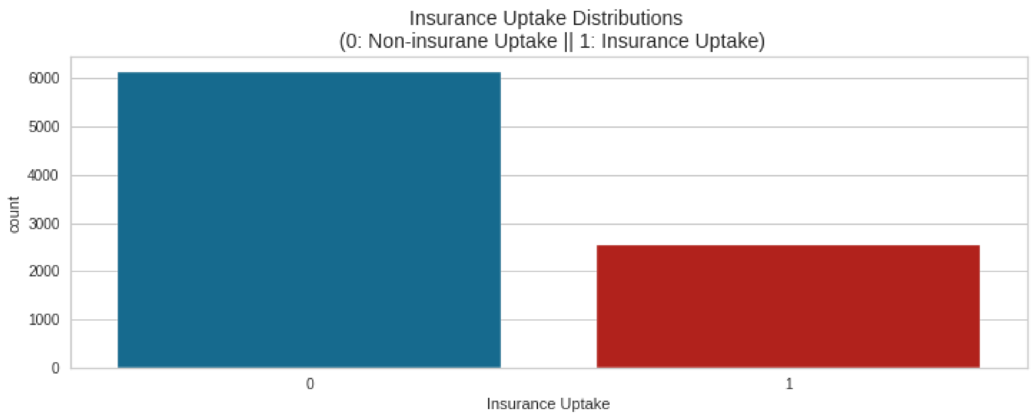
4.2. Comparison on Balanced Data

Table 2 shows the machine learning models and their respective precision scores, recall scores, F1-scores, and accuracy on the real unbalanced data, but with cross-validation test_size = 0.1 and validation_score = 0.15. Stratification was based on y, which is the insurance uptake in this case, with a set the random_for reproducibility. This stratifies the parameter by making a split so that the proportion of values in the sample produced will be the same as the proportion of values provided to the parameter; it ensures that in cross-validation, the skews within the folds are similar. High accuracy was observed among logistic, GBM, XGB, and SVM (0.84), then KNN and random forest (0.83), and finally, GNB and DT (0.77). On the other hand, for F1-scores, logistic had the highest (0.74), while the lowest was DT (0.65).
Table 3 shows the machine learning models and their respective precision scores, recall scores, F1-scores, and accuracy on the oversampled data. Random forest leads with the highest accuracy of 0.95 followed by DT (0.92), KNN (0.82), SVM (0.82), GBM and XGB (0.79), logistic regression (0.78), and lastly, GNB (0.74). However, upon hyperparameter tuning, the accuracy GBM and XGB increases. Nevertheless, random forest showed the highest precision score, recall score, F1-score, and accuracy; hence, it can be taken as the optimal model in this instance. Here, random forest is more robust than the other classifiers. This could be explained by it being an ensemble algorithm. The findings corroborate those of Han et al. [32], who asserted that ensemble algorithms tend to perform better than stand-alone algorithms. However, GBM and XGB give lower accuracy than the DT classifier, unlike our expectation. Hence, we could conclude that for this kind of oversampled data, ensemble trees by bagging tend to perform better than by boosting.
Table 4 shows the machine learning models and their respective precision scores, recall scores, F1-scores, and accuracy on the real downsampled data. The highest accuracy score was observed for XGB (0.87), then GBM (0.86), while the lowest was DT (0.72). For F1-scores, XGB had (0.87), then GBM (0.86), logistic (0.83), KNN, GNB, and random forest (0.82), and finally, DT (0.72). In the case of undersampled data, XGB and GBM showed higher accuracy than other models (0.87 and 0.86, respectively). Both of them are tree based ensemble learners, which are assembled by boosting. This allows us to construe that for the kind of data used, tree based learners assembled by boosting are more robust than others. This corroborates Golden et al. [25], who found GBM to perform better than other algorithms.
Despite being the same data source, the learners had different metrics for oversampled and undersampled data. The accuracy for the learners when the data were oversampled, vis à vis when undersampled, were: logistic (0.78, 0.83), GNB (0.74, 0.82), random forest (0.95, 0.82), DT (0.92, 0.72), SVM (0.82, 0.81), KNN (0.82, 0.82), GBM (0.79, 0.86), XGB (0.78, 0.87). This could imply that when the data were undersampled, the learners presumed different distributions from when oversampled, despite being the same data. However, SVM and KNN did not seem to show remarkable differences in accuracy when the data were either undersampled or oversampled.

4.3. Area under the Receiver Operating Characteristic Curves and Confusion Matrices

Upon imputing the optimized hyperparameters, the models were retrained, and AUCs and confusion matrices for the various models were drawn. Table 5 shows the values of TP, TN, FP, and FN that were extracted from the confusion matrices for various models. For TP, random forest led (190), then XGB (179), while KNN gave the least (150). This means that it is more likely for a random forest model to predict that one would take up insurance coverage and that that person does take up coverage compared to other models. For TN, DT was the highest (204), then random forest (201). For FN, DT was the lowest (1), then random forest (4), while logistic regression was the highest (51). For FP, random forest was the lowest (14), followed by XGB (25), while KNN and GNB were the highest (both 45). This implies that random forest is least likely to make type II errors in predicting uptake compared with other classifiers. Random forest seems to be the most robust since it had the highest true positives and the least false positives. Nevertheless, other tree based classifiers seemed to do well on the data.
Moreover, 
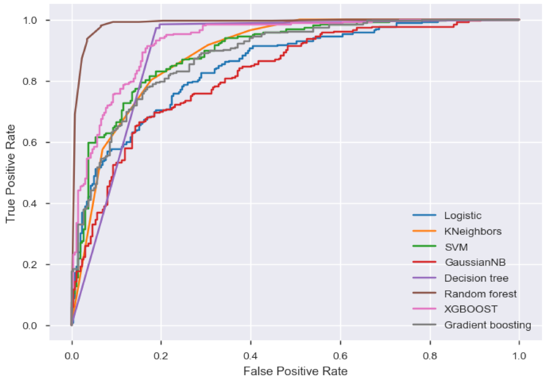
Figure 3 shows the areas under the receiver operating characteristics curve (AUCs) for the various models. The AUCs under the various models were: 0.8481 for logistic regression, 0.8914 for the K nearest neighbors classifier, 0.8220 for GNB, 0.8940 for SVM, 0.8962 for DT, 0.9866 for random forest, 0.9300 for XGB (referred to as XGBOOST in the figure), and 0.8823 for GBM. Based on the AUCs, random forest performed best compared to all other models since it gave the highest area under the receiver operating characteristics curve, followed by XGB classifier. This corroborates Blanco et al. [24], who found random forest to be a stronger model in the prediction of the efficiency of fullerene derivative based ternary organic solar cells. This implies that ensemble tree based models tend to perform better than others for this kind of data since both random forest and XGB are tree based models and are both ensemble algorithms.

4.4. Phase II Analysis: Comparison of Models on Oversampled Data

Phase II analysis involved using the 2019 FinAccess data with the Phase I analysis as the base. By taking Phase I analysis as the base, the two best models from Phase 1 were picked and compared with four deep learning classifiers. The deep learning classifiers were MLP, CNN, LSTM, and CNN-LSTM. Table 6 shows the precision score, recall score, F1-score, accuracy, and AUC for each of the respective models compared in the Phase II analysis. Random forest remained the most robust model for the insurance uptake prediction with the highest levels of the precision score, F1-score, accuracy, and AUC. However, the recall score was higher among the deep learning classifiers except for MLP. As found in Kim and Cho [26] and Sun et al. [27], the CNN-LSTM model showed better performance than the individual models CNN and LSTM separately.

4.5. Feature Importance

Feature importance in this study was employed to get an understanding of how the features contributed to the model predictions. As previously proposed by Casalicchio et al. [33], the effect of features, their respective contributions, as well as their respective attributions describe how and, to some degree, the extent to which each feature contributes to the prediction of the model. Furthermore, Pesantez-Narvaez et al. [34] added that the contribution of each feature to the outcome as given by the feature importance is based on Gini impurity. Feature importance was taken to identify important features that contribute to the greatest extent to the prediction of uptake. This enabled the analysis and comparison of the feature importance across various observations in the data. The feature importance was obtained from the random forest model, and since random forest is a tree based model, it gave the extent to which each feature contributed to reducing the weighted Gini impurity.
Based on the AUC and accuracy, random forest seemed to be the most robust in uptake prediction. Moreover, random forest showed the highest AUC, and hence, this model was used to extract the importance of each feature in the uptake prediction. Table 7 shows the feature importance from Phase I’s random forest model in predicting the insurance uptake. All the features show non-zero importance, but their rank from the most important to the least important is having a bank product, wealth quintile, subregion, level of education, age, group, most trusted provider, nature of residence, numeracy, household size, marital status, second most trusted provider, ownership of a phone, having a set emergency fund, having electricity as a light source, gender, nature of residential area, whether it is urban or rural, being a youth, and having a smartphone.
The result suggests that the most important factor is whether one has a bank product or not. This implies that individuals who have a bank product tend to have higher insurance uptake compared to those who do not. This could also imply that many individuals who had a bank product also had an insurance product. The second most important feature is the wealth quintile. This implies that the material wealth of an individual plays a critical role since the wealthier an individual, the higher would be the ability to pay for the insurance premiums. The ability to pay is a great factor in determining uptake. However, the potential loss of profit as a result of the misclassification of an insurance uptake client as non-uptake is higher than the potential loss of profit as a result of misclassifying non-uptake as an insurance uptake client. Hence, we suggest that cost-sensitive learning could be done based on these features, as was the case in Petrides et al. [12]. The subregion being the third factor could be construed to imply that the insurance products are not evenly distributed nationally. Interestingly, being a youth and having a smartphone did not show much importance in determining uptake, although much of the population is young. This could imply that the insurance products on the market are not appealing to youths, or they could be too expensive for them. More could be done on product engineering to make insurance products more affordable and more appealing so that more of the young populace could benefit from insurance.
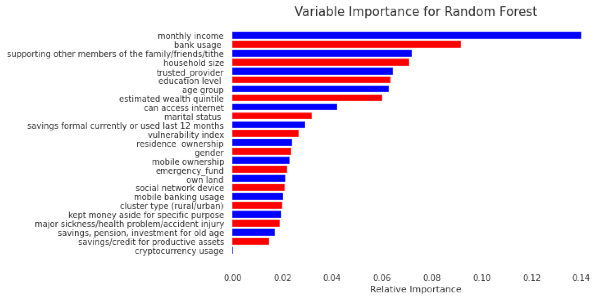
Figure 4 shows the feature importance as extracted from the Phase II analysis. Though bank usage is still an important feature in the prediction of insurance uptake, income has the highest contribution in reducing the weighted Gini impurity, implying that it is the most important feature. Other important factors include the willingness and ability to support others, household size, trusted financial service provider, age, and level of education. Unlike in the Phase I analysis, cryptocurrency usage had a non-zero contribution in the prediction of insurance uptake, though its contribution was least among the variables with non-zero contribution to the insurance uptake.

5. Conclusions and Recommendations

From Phase I, it could be construed that with the unbalanced data, the performance was lower compared to the performance on the balanced data. This could mean that the data imbalance problem is a significant contributor to poor model performance in insurance uptake prediction. Moreover, the learning metrics improved when the data were balanced by either oversampling the minority class (uptake of insurance for the case of the data used) or undersampling the majority class (non-uptake of insurance for the case of the data used). Therefore, alleviating data imbalance results in a more robust model in insurance uptake prediction. In the study, ensemble learners mostly tended to perform better than stand-alone algorithms. For oversampled data in Phase I, random forest, which is assembled by bagging, performed better than other machine learning classifiers that were considered. Random forest had the highest accuracy of 0.95. However, for undersampled data in Phase I, GBM and XGB, which are assembled by boosting, did better than the others. GBM and XGB had an accuracy of 0.87 and 0.86, respectively. Therefore, ensemble learners could be said to be the most robust for this kind of data. Moreover, random forest, GBM, and XGB are all tree based models; therefore, tree based ensemble machine learning models could be said to be robust for insurance uptake prediction. Likewise, in Phase II, the random forest model was most robust based on the F1-score, accuracy, precision, and the area under receiver operating characteristic curve. Furthermore, the CNN-LSTM model showed better performance compared to individual CNN and LSTM models. Despite being the same data source, the learners had different metrics for oversampled and undersampled data of the Phase I analysis. It could therefore be concluded that when the data are undersampled, the learners presume that they are drawn from different distributions from when they were oversampled, despite being the same data. However, SVM and KNN did not seem to show remarkable differences in accuracy when the data were either undersampled or oversampled. Further study could be done to find out if this lack of remarkable difference came by chance or if it stemmed from the nature of the classifiers. The most important feature in predicting uptake in Phase I was having a bank product. This could imply that bancassurance is a viable channel or the distribution of insurance products since the banked population is more likely to take up insurance. Income was most important in Phase II, while the wealth quintile was the second most important feature in Phase II. This, therefore, calls for insurance providers to come up with innovative products that would be affordable to the majority of the population. Spatial characteristics were the third most important factor in Phase II. This could imply that the distribution of insurance is not even in the nation. A further look at this could be done with multilevel modeling to establish the extent of the different levels of variation in the data. In recommending improvement from here, we suggest studies be done on specific lines of insurance with machine learning models that we have herein found to be most robust, in particular random forest. As the results suggest, there is a strong connection between the individual’s wealth and insurance uptake, so possible further work could include the use of cost-sensitive learning.

Author Contributions

N.K.Y. acquired the data, analyzed and prepared the draft manuscript. J.K., as a principal advisor for N.K.Y., advised and supervised the data acquisition, the analysis and the write-up of the manuscript. J.N., advised and supervised the analysis and the write-up of the manuscript. All authors read and approved the final manuscript.

Funding

This study was funded partly by the African Center of Excellence in Data Science and the University of Rwanda.

Institutional Review Board Statement

Not applicable.

Informed Consent Statement

Not applicable.

Data Availability Statement

Data used in Phase I analysis is publicly available dataset. It can be found in: https://doi.org/10.7910/DVN/JF8YST (accessed on 12 March 2021). Data used in Phase II is available upon request from KNBS at https://www.knbs.or.ke/?wpdmpro=2019-finaccess-household-survey (accessed on 12 March 2021).

Acknowledgments

We appreciate FinAccess, FSD, and KNBS for publicly providing the data used in this study.

Conflicts of Interest

The authors declare no conflict of interest.

Appendix A

Table A1. Hyperparameter optimization for RF.
ParameterRangeOptimal Value
n_estimators[80 to 150, interval of 10]110
max_features[auto, sqrt, log2]auto
min_samples_split[2, 4, 6, 8]2
Bootstrap[True, False]True
Table A2. Hyperparameter optimization for GBM.
ParameterRangeOptimal Value
n_estimators[100, 200, 300]100
min_samples learning_rate[0.01, 0.02, 0.05, 0.1]0.05
Table A3. Hyperparameter optimization for XGB.
ParameterRangeOptimal Value
n_estimators[500 to 1500]1000
max_depth[auto, sqrt, log2]auto
max_features[0.2 to 1]0.9
gamma[0.1 to 1]0.1
Table A4. Hyperparameter optimization for MLP.
Parameter RangeOptimal Value
n_Training epochs[100, 200, 300]300
max_Batch size[20, 40, 50, 100]50
max_Learning rate[0.0005, 0.001, 0.01]0.001
Activation function[softmax, ReLU]ReLU
Table A5. Hyperparameter optimization for CNN.
Parameter RangeOptimal Value
n_Training epochs[100, 200, 300]300
max_Batch size[20, 40, 50, 100]40
max_Learning rate[0.0005, 0.001, 0.01]0.001
Activation function[softmax, ReLU]ReLU
Table A6. Hyperparameter optimization for LSTM.
Parameter RangeOptimal Value
n_Training epochs[100,200,300]300
max_Batch size[20, 40,50, 100]50
max_Learning rate[0.0005,0.001,0.01]0.001
Activation function[softmax, ReLU]ReLU
Table A7. Hyperparameter optimization for CNN-LSTM.
Parameter RangeOptimal Value
n_Training epochs[100, 200, 300]300
max_Batch size[20, 40, 50, 100]40
max_Learning rate[0.0005, 0.001, 0.01]0.001
Activation function[softmax, ReLU]ReLU

References

  1. Olayungbo, D.; Akinlo, A. Insurance penetration and economic growth in Africa: Dynamic effects analysis using Bayesian TVP-VAR approach. Cogent Econ. Financ. 2016, 4, 1150390. [Google Scholar] [CrossRef] [Green Version]
  2. Zhou, J.; Guo, Y.; Ye, Y.; Jiang, J. Multi-Label Entropy-Based Feature Selection with Applications to Insurance Purchase Prediction. In Proceedings of the 2020 IEEE International Conference on Artificial Intelligence and Computer Applications (ICAICA), Dalian, China, 27–29 June 2020; pp. 427–432. [Google Scholar]
  3. African Union Commission. Agenda2063-The Africa We Want; African Union Commission: Addis Ababa, Ethiopia, 2017. [Google Scholar]
  4. Lambregts, T.R.; Schut, F.T. A Systematic Review of the Reasons for Low Uptake of Long-Term Care Insurance and Life Annuities: Could Integrated Products Counter Them? Netspar: Tilburg, The Netherlands, 2019. [Google Scholar]
  5. AKI. Insurance Industry Annual Report 2015; Technical Report; Association of Kenya Insurers: Nairobi City, Kenya, 2015. [Google Scholar]
  6. Gine, X.; Ribeiro, B.; Wrede, P. Beyond the S-Curve: Insurance Penetration, Institutional Quality and Financial Market Development; The World Bank: Washington, DC, USA, 2019. [Google Scholar] [CrossRef]
  7. Venderley, J.; Khemani, V.; Kim, E.A. Machine learning out-of-equilibrium phases of matter. Phys. Rev. Lett. 2018, 120, 257204. [Google Scholar] [CrossRef] [Green Version]
  8. López Belmonte, J.; Segura-Robles, A.; Moreno-Guerrero, A.J.; Parra-González, M.E. Machine learning and big data in the impact literature. A bibliometric review with scientific mapping in Web of science. Symmetry 2020, 12, 495. [Google Scholar] [CrossRef] [Green Version]
  9. Grize, Y.L.; Fischer, W.; Lützelschwab, C. Machine learning applications in nonlife insurance. Appl. Stoch. Model. Bus. Ind. 2020, 36, 523–537. [Google Scholar] [CrossRef]
  10. Krah, A.S.; Nikolić, Z.; Korn, R. Machine learning in least-squares Monte Carlo proxy modeling of life insurance companies. Risks 2020, 8, 21. [Google Scholar] [CrossRef] [Green Version]
  11. Bärtl, M.; Krummaker, S. Prediction of claims in export credit finance: A comparison of four machine learning techniques. Risks 2020, 8, 22. [Google Scholar] [CrossRef] [Green Version]
  12. Petrides, G.; Moldovan, D.; Coenen, L.; Guns, T.; Verbeke, W. Cost-sensitive learning for profit-driven credit scoring. J. Oper. Res. Soc. 2020, 1–13. [Google Scholar] [CrossRef]
  13. Aghabozorgi, S.; Shirkhorshidi, A.S.; Wah, T.Y. Time-series clustering–a decade review. Inf. Syst. 2015, 53, 16–38. [Google Scholar] [CrossRef]
  14. Pavlyshenko, B.M. Machine-learning models for sales time series forecasting. Data 2019, 4, 15. [Google Scholar] [CrossRef] [Green Version]
  15. Dashtipour, K.; Gogate, M.; Adeel, A.; Ieracitano, C.; Larijani, H.; Hussain, A. Exploiting deep learning for Persian sentiment analysis. In Proceedings of the International Conference on Brain Inspired Cognitive Systems, Xi’an, China, 7–8 July 2018; pp. 597–604. [Google Scholar]
  16. Jain, A.K. Data clustering: 50 years beyond K-means. Pattern Recognit. Lett. 2010, 31, 651–666. [Google Scholar] [CrossRef]
  17. Tkáč, M.; Verner, R. Artificial neural networks in business: Two decades of research. Appl. Soft Comput. 2016, 38, 788–804. [Google Scholar] [CrossRef]
  18. Sundarkumar, G.G.; Ravi, V. A novel hybrid undersampling method for mining unbalanced datasets in banking and insurance. Eng. Appl. Artif. Intell. 2015, 37, 368–377. [Google Scholar] [CrossRef]
  19. Shalev-Shwartz, S.; Ben-David, S. Understanding Machine Learning: From Theory to Algorithms; Cambridge University Press: Cambridge, UK, 2014. [Google Scholar]
  20. Huang, S.; Cai, N.; Pacheco, P.P.; Narrandes, S.; Wang, Y.; Xu, W. Applications of support vector machine (SVM) learning in cancer genomics. Cancer Genom.-Proteom. 2018, 15, 41–51. [Google Scholar]
  21. Naganandhini, S.; Shanmugavadivu, P. Effective Diagnosis of Alzheimer’s Disease using Modified Decision Tree Classifier. Procedia Comput. Sci. 2019, 165, 548–555. [Google Scholar] [CrossRef]
  22. Olanow, C.W.; Koller, W.C. An algorithm (decision tree) for the management of Parkinson’s disease: Treatment guidelines. Neurology 1998, 50, S1. [Google Scholar] [CrossRef]
  23. Muniyandi, A.P.; Rajeswari, R.; Rajaram, R. Network anomaly detection by cascading k-Means clustering and C4. 5 decision tree algorithm. Procedia Eng. 2012, 30, 174–182. [Google Scholar] [CrossRef] [Green Version]
  24. Blanco, C.M.G.; Gomez, V.M.B.; Crespo, P.; Ließ, M. Spatial prediction of soil water retention in a Páramo landscape: Methodological insight into machine learning using random forest. Geoderma 2018, 316, 100–114. [Google Scholar] [CrossRef]
  25. Golden, C.E.; Rothrock, M.J., Jr.; Mishra, A. Comparison between random forest and gradient boosting machine methods for predicting Listeria spp. prevalence in the environment of pastured poultry farms. Food Res. Int. 2019, 122, 47–55. [Google Scholar] [CrossRef] [Green Version]
  26. Kim, T.Y.; Cho, S.B. Predicting residential energy consumption using CNN-LSTM neural networks. Energy 2019, 182, 72–81. [Google Scholar] [CrossRef]
  27. Sun, J.; Di, L.; Sun, Z.; Shen, Y.; Lai, Z. County-level soybean yield prediction using deep CNN-LSTM model. Sensors 2019, 19, 4363. [Google Scholar] [CrossRef] [Green Version]
  28. Central Bank of Kenya; FSD Kenya; Kenya National Bureau of Statistics. FinAccess Household Survey 2015; Central Bank of Kenya: Nairobi, Kenya, 2016. [Google Scholar] [CrossRef]
  29. Amin, A.; Anwar, S.; Adnan, A.; Nawaz, M.; Howard, N.; Qadir, J.; Hawalah, A.; Hussain, A. Comparing oversampling techniques to handle the class imbalance problem: A customer churn prediction case study. IEEE Access 2016, 4, 7940–7957. [Google Scholar] [CrossRef]
  30. Pawluszek-Filipiak, K.; Borkowski, A. On the Importance of Train–Test Split Ratio of Datasets in Automatic Landslide Detection by Supervised Classification. Remote Sens. 2020, 12, 3054. [Google Scholar] [CrossRef]
  31. Poria, S.; Cambria, E.; Hazarika, D.; Majumder, N.; Zadeh, A.; Morency, L.P. Context-dependent sentiment analysis in user-generated videos. In Proceedings of the 55th Annual Meeting of the Association for Computational Linguistics (Volume 1: Long Papers), Vancouver, BC, Canada, 30 July–4 August 2017; pp. 873–883. [Google Scholar]
  32. Han, T.; Siddique, A.; Khayat, K.; Huang, J.; Kumar, A. An ensemble machine learning approach for prediction and optimization of modulus of elasticity of recycled aggregate concrete. Constr. Build. Mater. 2020, 244, 118271. [Google Scholar] [CrossRef]
  33. Casalicchio, G.; Molnar, C.; Bischl, B. Visualizing the feature importance for black box models. In Proceedings of the Joint European Conference on Machine Learning and Knowledge Discovery in Databases, Dublin, Ireland, 10–14 September 2018; pp. 655–670. [Google Scholar]
  34. Pesantez-Narvaez, J.; Guillen, M.; Alcañiz, M. Predicting motor insurance claims using telematics data—XGBoost versus logistic regression. Risks 2019, 7, 70. [Google Scholar] [CrossRef] [Green Version]
Figure 1. Data imbalance Phase I.
Data 06 00116 g001
Figure 2. Data imbalance Phase II.
Data 06 00116 g002
Figure 3. Areas under the receiver operating characteristics curve (AUCs).
Data 06 00116 g003
Figure 4. Phase II variable importance.
Data 06 00116 g004
Table 1. Machine learning models’ performance on the unbalanced data.
NumberModelPrecisionRecallF1-ScoresAccuracy
0Logistic0.68550.54300.60600.8485
1GNB0.45760.72580.56130.7565
2Random Forest0.63010.39070.48230.8200
3DT0.43390.48210.45670.7538
4SVM0.72650.48570.58220.8504
5KNN0.57810.49100.53100.8138
6GBM0.70540.51080.59250.8492
7XGB0.72040.51260.59900.8527
Table 2. Machine learning models’ performance on the unbalanced data with cross-validation.
NumberModelPrecisionRecallF1-ScoresAccuracy
0Logistic0.77260.72280.74230.8442
1GNB0.69120.75070.70590.7712
2Random Forest0.74560.67480.69770.8269
3DT0.64740.64930.64830.7654
4SVM0.77040.68090.70800.8365
5KNN0.74950.71550.72970.8327
6GBM0.77200.71150.73380.8423
7XGB0.76300.69440.71820.8366
Table 3. Machine learning models’ performance on the oversampled data.
NumberModelPrecisionRecallF1-ScoresAccuracy
0Logistic0.77750.77760.77750.7775
1GNB0.74400.74360.74320.7433
2Random Forest0.94930.94670.94620.9462
3DT0.93110.92500.92400.9242
4SVM0.81930.81920.81910.8191
5KNN0.83280.82500.82310.8240
6GBM0.79210.79220.79220.7922
7XGB0.78740.78740.78730.7873
Table 4. Machine learning model performance on the downsampled data.
NumberModelPrecisionRecallF1-ScoresAccuracy
0Logistic0.82920.83140.82970.8303
1GNB0.82000.82160.82050.8214
2Random Forest0.82070.82320.82190.8214
3DT0.72100.72020.72050.7232
4SVM0.81250.81500.81210.8125
5KNN0.82070.82320.82090.8214
6GBM0.85580.85760.85640.8571
7XGB0.86490.86740.86550.8661
Table 5. Confusion matrices.
NumberModelTPTNFPFN
0Logistic1641544051
1GNB1591914514
2Random Forest190201144
3DT170204341
4SVM1581914614
5KNN1591914514
6GBM1691663537
7XGB1791902515
Table 6. Machine learning models’ performance for the oversampled data.
NumberModelPrecisionRecall ScoreF1-ScoresAccuracyAUC
0Random Forest0.941750.938630.939320.939530.98620
1XGBoost0.886450.879600.880400.881210.92690
2MLP0.829270.714290.767490.777540.85210
3CNN0.861420.966390.910890.902810.95113
4LSTM0.874050.962190.916000.909290.95592
5CNN-LSTM0.880310.957980.917510.911450.95666
Table 7. Feature importance.
RankFeatureImportance
1Having a bank product0.191
2Wealth quintile0.111
3Subregion0.109
4Education0.088
5Age group0.068
6Most trusted provider0.051
7Nature of residence0.050
8Numeracy0.048
9Household size0.047
10Marital status0.041
112nd most trusted provider0.039
12Ownership of a phone0.038
13Having a set emergency fund0.033
14Having electricity as a light source0.031
15Gender0.030
16Urban vs. rural0.026
17Being a youth0.026
18Having a smartphone0.023
Publisher’s Note: MDPI stays neutral with regard to jurisdictional claims in published maps and institutional affiliations.

