Use of the WRF-DA 3D-Var Data Assimilation System to Obtain Wind Speed Estimates in Regular Grids from Measurements at Wind Farms in Uruguay

Abstract

This work assessed the quality of wind speed estimates in Uruguay. These estimates were obtained using the Weather Research and Forecast Model Data Assimilation System (WRF-DA) to assimilate wind speed measurements from 100 m above the ground at two wind farms. The quality of the estimates was assessed with an anemometric station placed between the wind farms. The wind speed estimates showed low systematic errors at heights of 87 and 36 m above the ground. At both levels, the standard deviation of the total errors was approximately 25% of the mean observed speed. These results suggested that the estimates obtained could be of sufficient quality to be useful in various applications. The assimilation process proved to be effective, spreading the observational gain obtained at the wind farms to lower elevations than those at which the assimilated measurements were taken. The smooth topography of Uruguay might have contributed to the relatively good quality of the obtained wind estimates, although the data of only two stations were assimilated, and the resolution of the regional atmospheric simulations employed was relatively low.

1. Summary

This work evaluated the use of techniques for assimilation of data from field measurements into initial conditions of atmospheric numerical simulations in order to obtain wind estimates in Uruguay, at heights of 100 m above the ground and lower. The wind was estimated with hourly frequency in a regular grid that covers the country. The field data to be assimilated was operatively measured in wind farms installed in Uruguay, using anemometers placed 100 m above the ground. The data was assimilated into initial conditions for the Weather Research and Forecast regional model (WRF) of the National Center of Atmospheric Research (NCAR), [1] using the module for data assimilation included in this model, the WRF-DA module [2].

The data assimilation process, also called analysis, is an essential component of numerical atmospheric forecasts, and its main purpose is to generate initial conditions for the predictions. The variables that compose an initial condition are called prognostic variables because the model uses their values at a given instant to compute their values at a later time. To generate an initial condition for a specific numerical model at a given time, a first approximation is generally used. This first approximation, called “background condition”, usually consists of a prediction for the same instant, obtained with the same model, from previous initial conditions. The data assimilation system must combine the information from the background condition with the information from measurements of atmospheric variables (or variables of systems related to it; for example, the ocean, the soil, or the cryosphere). This combination of information is done in a way that optimizes the quality of the result in statistical terms, either minimizing the expected value of the sum of its quadratic errors or maximizing its likelihood. Note that the short-term predictions used as background values are, in turn, affected by field measurements that were assimilated during previous times. This allows considering information from regions or atmospheric levels in which few measurements are available since measurements, done earlier in other regions or at other levels, can propagate their influence through atmospheric dynamical processes into the zones that have relatively fewer observations.

Kalnay [3] described the main techniques for data assimilation that are currently used, such as optimal interpolation, 3D-Var, Kalman filters, ensemble Kalman filters, and 4D-Var. The WRF-DA system implements the 3D-Var [4] and 4D-Var techniques [5], and a technique that combines the ensemble Kalman filter with 3D-Var [6,7]. Harlim [8] pointed that the referred techniques assume that the errors from the background conditions and the field measurements are unbiased and normally distributed, although numerical models inevitably have systematic errors. These assumptions can provide reasonable estimates of the first-order statistics while being practical to implement. However, these methodologies require caution for interpreting their higher-order statistical estimates, and an important challenge in data assimilation is to use existing methods in the presence of model systematic errors. The author proposed methodologies to mitigate the effects of model systematic errors on the results of the assimilation process. Rao and Sandu [9] proposed an a-posteriori error estimation methodology that quantifies the impact of model and data errors on the inference results of inverse problems, including the 4D-Var assimilation process. The model and data errors considered include both unbiased noise and systematic biases. The authors found that the proposed methodology could be useful to reduce and quantify uncertainties in a real-time system with feedback. Besides, the error estimates can be used to locate faulty sensors and to determine areas of maximum sensitivity, where improvements in the stations network or an increase in model resolution may be required.

In addition to its direct use in the numerical prediction process, the results of data assimilation can be considered “pseudo-observations” of atmospheric variables in regular grids. Note that these do not consist purely of interpolations of field measurements in a regular grid since they also consider the information from short-term predictions. The uses of the pseudo-observations obtained from a data assimilation process can be very broad, but they require an evaluation of their quality by comparison with field measurements not used in the assimilation process.

The current work used the rather conventional 3D-Var assimilation technique. In Section 2, we described the data used, both from field measurements and from numerical predictions used as background conditions, and we referred to the quality control method used for the field data from the wind farms. In Section 3, we described the main aspects of the 3D-Var assimilation technique and its implementation in this work using the WRF DA system. In Section 4, we described the main results, and in Section 5, we presented the conclusions.

2. Data Description

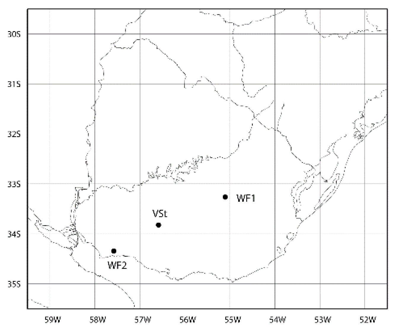
The wind data used in the data assimilation process was obtained from two anemometers installed in the “Rosendo Mendoza” (WF1) and “Valentines” (WF2) wind farms. The geographic locations of these wind farms are shown in Figure 1. The anemometers were placed 100 m above the ground, and they recorded mean velocities for successive periods of 15 min, which were transmitted to the National Dispatch of Electric Charges of Uruguay, operated by the Electricity Market Administration (Administración del Mercado Eléctrico; ADME) and the National Administration of Electric Power Plants and Transmissions (Usinas y Trasmisiones del Estado; UTE), and Uruguayan National Public Electricity Utility Organizations. In addition to the wind measurements, the mean electric power generated in the same 15-min periods and the corresponding quantity of aerogenerators that were effectively active were also transmitted by each wind farm. These additional data allowed for a quality control analysis of the measurements, as described by Orteli and Cazes Boezio [10]. With the historical information of wind velocity and electric power generated, the authors built an empirical wind-power curve for each wind farm. In those cases in which not all the aerogenerators of the wind farm were active, the power generation that would correspond to a condition of full availability was estimated by linear extrapolation. The authors considered that those combinations of wind and generated power that depart from the empirical curve beyond certain thresholds were suspicious of being affected by malfunctioning of the measurement or recording systems, or by occasional interference of the wake of an aerogenerator with the anemometer. The data from WF1 and WF2 available for this study were from the months from January to May and from November to December of 2017 (seven months).

To evaluate the quality of the pseudo-observations obtained through the implemented data assimilation process, an independent station was used (“validation station”, VSt), which is located at Colonia Arias, Uruguay. The station location is also shown in Figure 1. The station measures wind speed and direction at heights of 87 and 36 m above the ground and is part of a network of stations that measures wind velocity and solar radiation that has been operated by UTE since 2009. This network is described by Cornalino and Draper [11], and its measurements (that include wind velocities averaged every 10 min) are made available online by UTE. In recent years, many of the anemometric stations operated by UTE have become affected by wind farms. The VSt of Colonia Arias has been active since 2011, and during the period studied in this work, it was not affected by any wind farm. 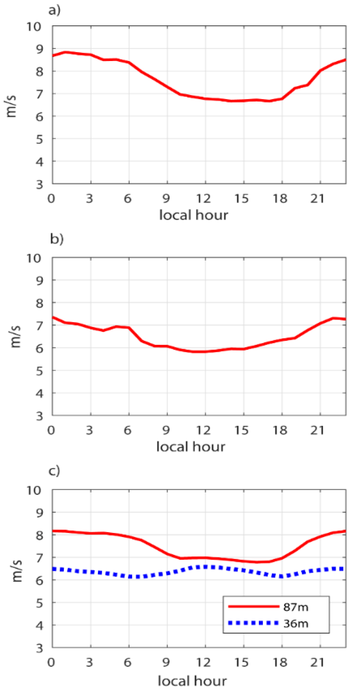Figure 2 shows the wind speed at the WF1, WF2, and Vst sensors averaged for each local hour during the seven months considered.

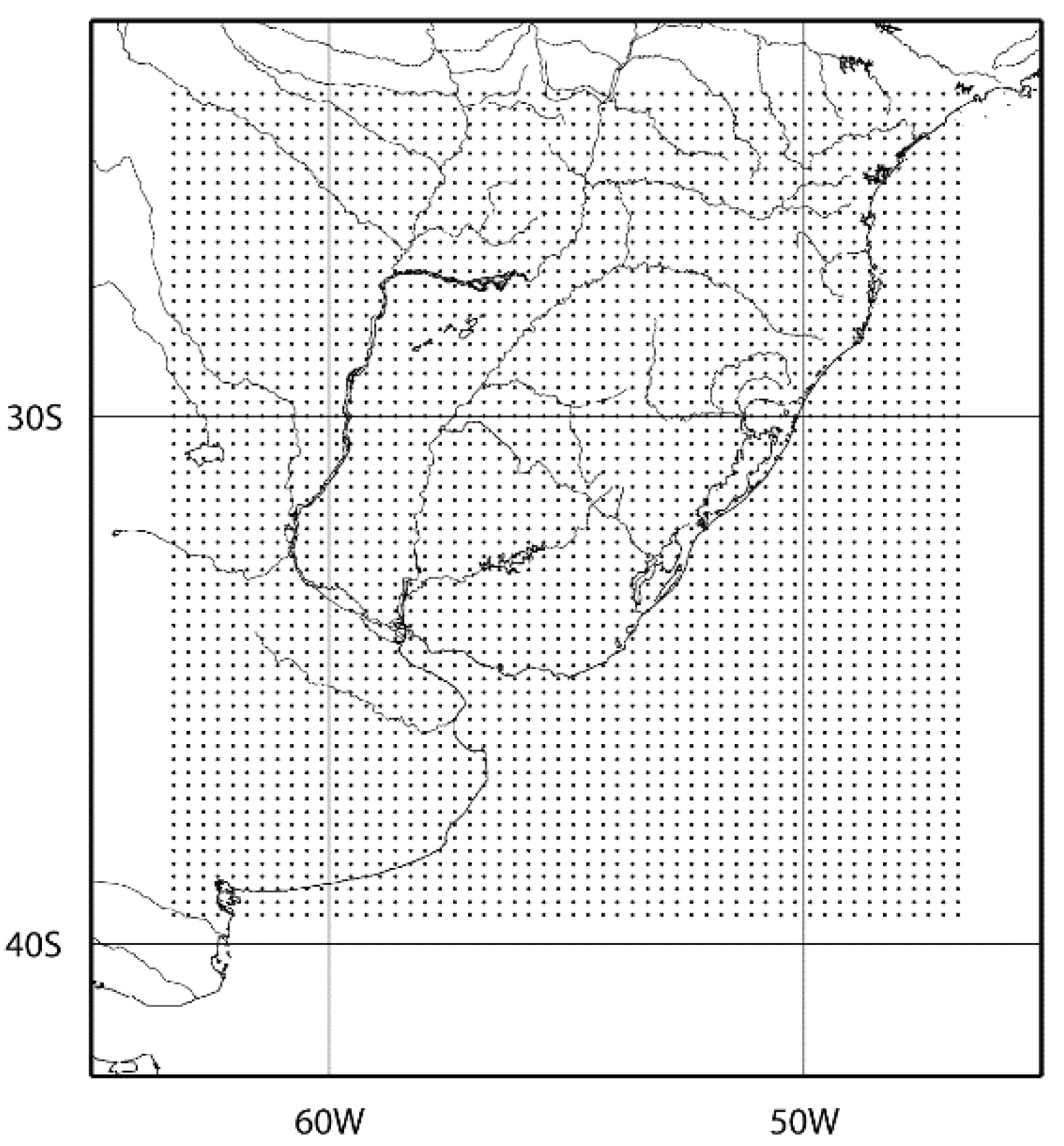
The assimilation process uses regional simulations computed with the WRF model from NCAR, as shown by Cazes Boezio and Orteli [12]. The regional simulations take their initial and boundary conditions from global predictions made by the Global Forecast System (GFS) of the National Ocean and Atmosphere Administration (NOAA) of the Unites States. The horizontal grid of the regional simulations has a resolution of 30 km in the zonal and meridional directions, as shown in Figure 3. The vertical direction is discretized in 54 levels, 7 of which are within the first 100 m of height above the ground. In Appendix A, we indicated the parameterizations of physical processes employed, and we defined in detail the vertical discretization. The regional simulations have two purposes: first, they generate the background conditions into which the data measured in WF1 and WF2 are assimilated; and second, they allow for the estimation of the matrix of covariances of the errors of these background conditions. In Section 3, the hours of initialization and the simulated periods used for each one of these purposes were specified.

3. Methods

Next, we described the main aspects of the 3D-Var assimilation technique, which was used in this work and is available in the WRF-DA system. A complete description of this technique and its implementation in the WRF-DA system can be found in the NCAR Technical Note 453 [13], in Barker et al. [4] and Barker et al. [2], while the corresponding operational details are given in the WRF-DA User Guide [14].

The background condition information is displayed as a vector called x_b, which contains the values of all the different prognostic variables that compose the background condition in a certain conventional order. This information is displayed for each variable and each point of the grid. The field measurements that are to be assimilated, obtained at the same instant that corresponds to x_b, are displayed as a vector called y, also in a conventional order. The initial condition determined by the assimilation system is expressed as a vector called x_a, with a structure analogous to that of x_b. x_a combines the information from the background condition x_b and the field measurements contained in y, as expressed in Section 1. The 3D-Var technique determines the vector x_a as that of maximum likelihood, conditioned to the information of the background condition and the field measurements, and is the vector x that minimizes the following expression [3]:

$$J\left(x\right)=\frac{1}{2}{\left(x-x_b\right)}^T{B}^{-1}\left(x-x_b\right)+\frac{1}{2}{\left(y-H\left(x\right)\right)}^T{R}^{-1}\left(y-H\left(x\right)\right)$$

(1)

that is, $J\left(x_a\right)$ must be minim. In this formula, B and R are the matrices of error covariances of the background condition x_b and the field measurements y, respectively. It is assumed that these errors are normal variables and are unbiased. The B matrix is thus related to the accidental errors of x_b, while the model systematic errors or biases are assumed to be zero, as pointed out in [8]. Matrix B is defined as follows:

$$B\equiv E\left(\left(x_b-x_t\right)·{\left(x_b-x_t\right)}^T\right)$$

(2)

where E represents the expected value of the elements of the matrix $\left(x_b-x_t\right)·{\left(x_b-x_t\right)}^T$, and x_t is the vector of the true values of the variables contained in x_b. Note the actual values of x_t are unknown, so it becomes necessary to define a technique to estimate the values of B from available information.

H(x) is an operator that yields results analogous to the variables y from the model prognostic variables included in x. As an example, if an element of y represents the measurement of the meridional wind at a certain geographical location and a certain height, H(x) interpolates the values of the meridional wind field obtained from the numerical model at the geographical location and the height of this measurement. The H operator is generally non-linear, but it is possible to linearize it with the following approximation:

$$H\left(x\right)=H\left(x_b+x-x_b\right)\approx H\left(x\right)+\nabla H\left(x-x_b\right),$$

(3)

where ∇H is the gradient of H(x). If the linearized expression for H(x) is used, J(x) assumes a quadratic form.

It is assumed that the errors of the field measurements contained in vector y are statistically independent of each other, so R is a diagonal matrix; its diagonal contains the variances of the errors of each field measurement.

The matrix B is essential to this assimilation system. First, its non-diagonal terms contain the covariances of x_b errors at different grid points and also the covariances of errors of different variables. These covariances are necessary to propagate the information related to any field measurement through the horizontal and vertical directions and allow measurement of a specific variable to affect the analysis of others. In addition to this, the matrices B⁻¹ and R⁻¹ together determine the relative importance of the background conditions x_b and the field measurements y to determine the analysis x_a.

The WRF-DA system offers two methods to estimate B: the National Meteorological Center method (NMC), described by Parrish and Derber [15], and a method based on ensembles of predictions ([1], Chapter 9). Due to the availability of computer resources, we used the NMC method, which is relatively more economic. This method requires a database of pairs of x_b; each pair has two short-term predictions for the same hour obtained with different forecast horizons (for example, 12 and 24 h), and consequently with different initial conditions. The pairs of predictions correspond to certain hours of the day (for example, 0:00 and 12:00 GMT), and cover a certain period (for example, one year). It is assumed that the differences between the forecasts of each pair have statistical properties analogous to those of the background condition errors, and in particular, to estimate B, the following approximation can be used:

$$B=E\left({\left(x_b-x_t\right)}^T·\left(x_b-x_t\right)\right)\approx E\left({\left(x_b^{12hs}-x_b^{24hs}\right)}^T·\left(x_b^{12hs}-x_b^{24hs}\right)\right)$$

(4)

where $x_b^{12hs}$ and $x_b^{24hs}$ are a generic pair of predictions with 12 and 24 h time horizons, respectively. The validation of this technique to estimate B is empirical.

Note that, if n is the length of the x_a, and x_b vectors, the size of B is nxn. This implies a matrix of very large dimensions that would cause important technical difficulties to operate with B or B⁻¹, and even to store them in the computer memory. The 3D-Var technique implemented in the WRF-DA system solves this problem by factoring B as a product of certain matrices that have clear physical interpretations, allowing certain assumptions about their structures to be made and making them computationally tractable [2,4].

As a final remark in this subsection, we noted that both for the simulations of the background conditions and the estimation of the B matrix, a specific configuration of the WRF model was used, which here is the one described in Section 2.

WRF-DA Implementation for This Work

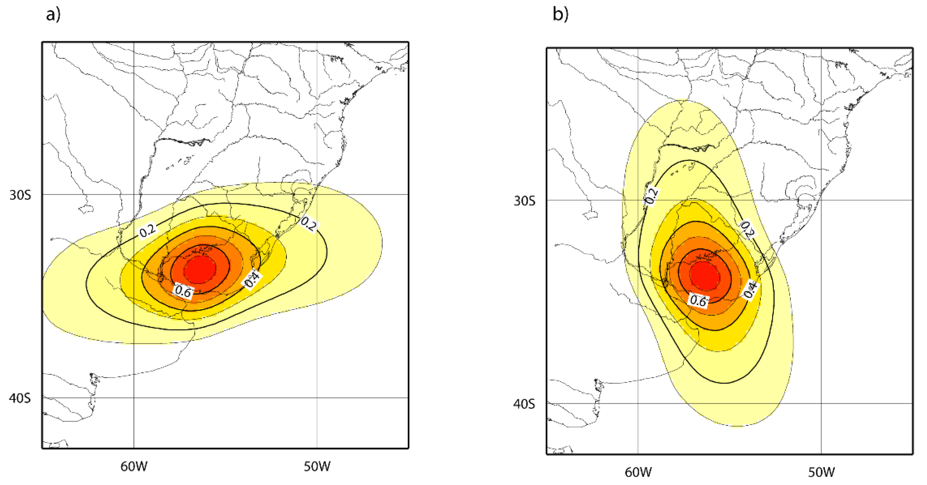
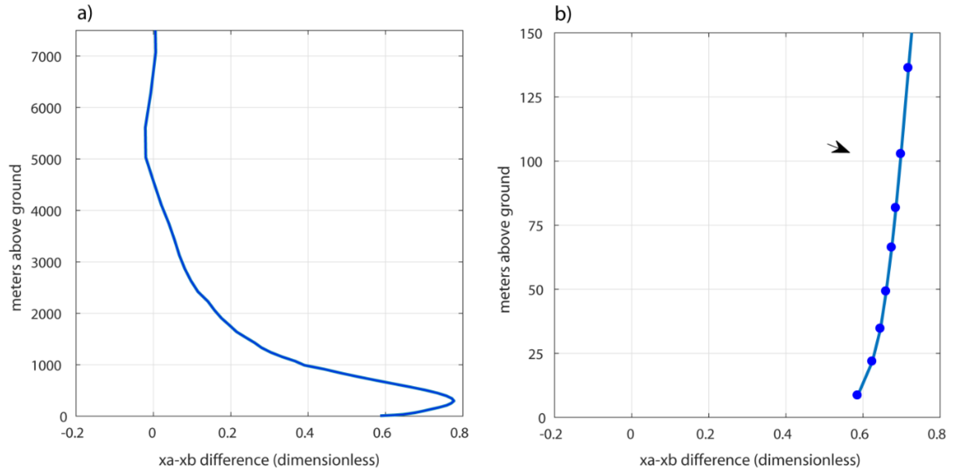
To apply the NMC method to estimate the matrix B, we used WRF-GFS simulations extended for 24 h and initialized at 0:00 GMT and 12:00 GMT during the entire year of 2016. The results obtained for 12 and 24 h after the initial conditions were used to estimate the matrix B, as indicated in the previous section. In order to gain insight into the spatial structure of the covariances contained in B, Decombes et al., [16] and Rivi [17] proposed “pseudo-single observation tests”. Such tests consist of choosing a particular variable of x_b in a particular grid point and suppose a hypothetical observation that increments in a fixed amount the background value of this variable at the selected grid point. The data assimilation process is carried on considering this single pseudo observation and prescribing a hypothetical value of the standard deviation of its error. Rivi [17] showed that the x_a − x_b difference was proportional to the covariance between the errors of the background variable in question at the chosen grid point and the errors of the rest of the background variables at all the grid points. The plots of the x_a − x_b differences for selected variables illustrate how the B matrix spreads the information of field measurements. In Appendix B, we summarized the fundamentals of the pseudo observation tests, and we showed some selected results for the B matrix estimated here.

The background conditions x_b were obtained from WRF-GFS simulations initiated at 0:00, 6:00, 12:00, and 18:00 GMT, during those months of 2017 for which information from the WF1 and WF2 stations was available. We used the hourly results of these simulations from 4 to 9 h since the initialization of each simulation. In this way, four consecutive simulations could cover the 24 h of each day. The selected forecast horizon was the earliest for which the GFS prediction results were available in real-time, with some time left to carry out the processes described in this work. In this way, it is possible to implement these processes in an operative mode. For each local hour in Uruguay,

Table 1. Hours within the WRF simulations used to define the background conditions as a function of the initialization cycle and local time in Uruguay. Each row corresponds to an initialization cycle, and each column corresponds to a local hour in Uruguay. The hours used within each cycle are indicated, considering the hours elapsed since its initialization.

	Local UY Hour
Initialization Cycle	0*	1	2	3	4	5	6	7	8	9	10	11	12	13	14	15	16	17	18	19	20	21	22	23
0:00		4	5	6	7	8	9
6:00								4	5	6	7	8	9
12:00														4	5	6	7	8	9
18:00	9*																			4	5	6	7	8

*: Local time 0 uses the results at the ninth hour of the simulation started at 18:00 GMT on the previous day as a background condition.

shows which WRF-GFS initialization cycle was used, and which hour within its forecast horizon corresponded to the background condition for that local hour.

In the present study, the assimilation made for each hour was independent of the previous assimilations; the corresponding background condition only incorporated information from the GFS global simulation. This is called a “cold start”. Alternatively, the background conditions could also have considered the field measurements made in previous hours. This alternative is called a warm start. The warm start method was tested in the context of the present work and obtained results of equivalent quality to those obtained with the cold start, so here we showed only the latter results. The similarity of the results from both methods might be because the assimilated information was very local; the assimilation of data in a wider region could influence the simulations in the area of interest over more hours and thus increase the relevance of assimilation from previous hours. The verification of this hypothesis requires a database of field measurements more complete than the one that was available for this work.

Each field measurement is specified to the WRF-DA system in a file that contains the day and time of the measurement, the geographic coordinates, and ground elevation of the corresponding station, the height of the measurement sensor, and the records of wind speed and direction. This information is used to generate the vector of field observations, y. Considering that the topography of the regional model has some degree of smoothing, the elevation of the specified terrain is not the actual elevation, but the elevation corresponding to the topography of the model interpolated to the station’s location coordinates. The height specified for the sensors is the elevation of the station plus 100 m. The specified module of wind speed is the average of the anemometer record for two consecutive 15-min periods centered on the hour for which the assimilation will be performed.

The specified wind direction is deduced from the background condition, interpolating each component of the wind vector to the geographical position and elevation of the anemometer. Although vanes are available at the stations, it was found that using their records produces results that are not as satisfactory as those obtained by deducing the wind direction from the background condition. This suggests that the quality of data obtained from these weathervanes is relatively poor, while regional short-term predictions are reasonably good with regard to this variable. It may be of interest to evaluate the effect of the assimilation of atmospheric pressure measurements on the wind direction obtained in the analysis, but no such observations were available to complete this analysis.

In addition, to estimate the R matrix, the WRF-DA system uses a file that specifies the standard deviations of the errors of the different kinds of field observations (obserr.txt). In the present work, we adjusted the errors specified in this file, proposing a value of 0.1 m/s for wind speed, which is reasonable for the type of sensors installed in the stations considered here [18]. For wind direction, we kept the default value proposed in the obserr.txt file, 5°. We also pointed out that the WRF-DA system uses two “namelist” files to prescribe parameters to be set for the B matrix estimation and the computation of the resultant analysis (x_a vector). In this work, we used the default values for these parameters, which are indicated in the WRF-DA user guide [14].

4. Results

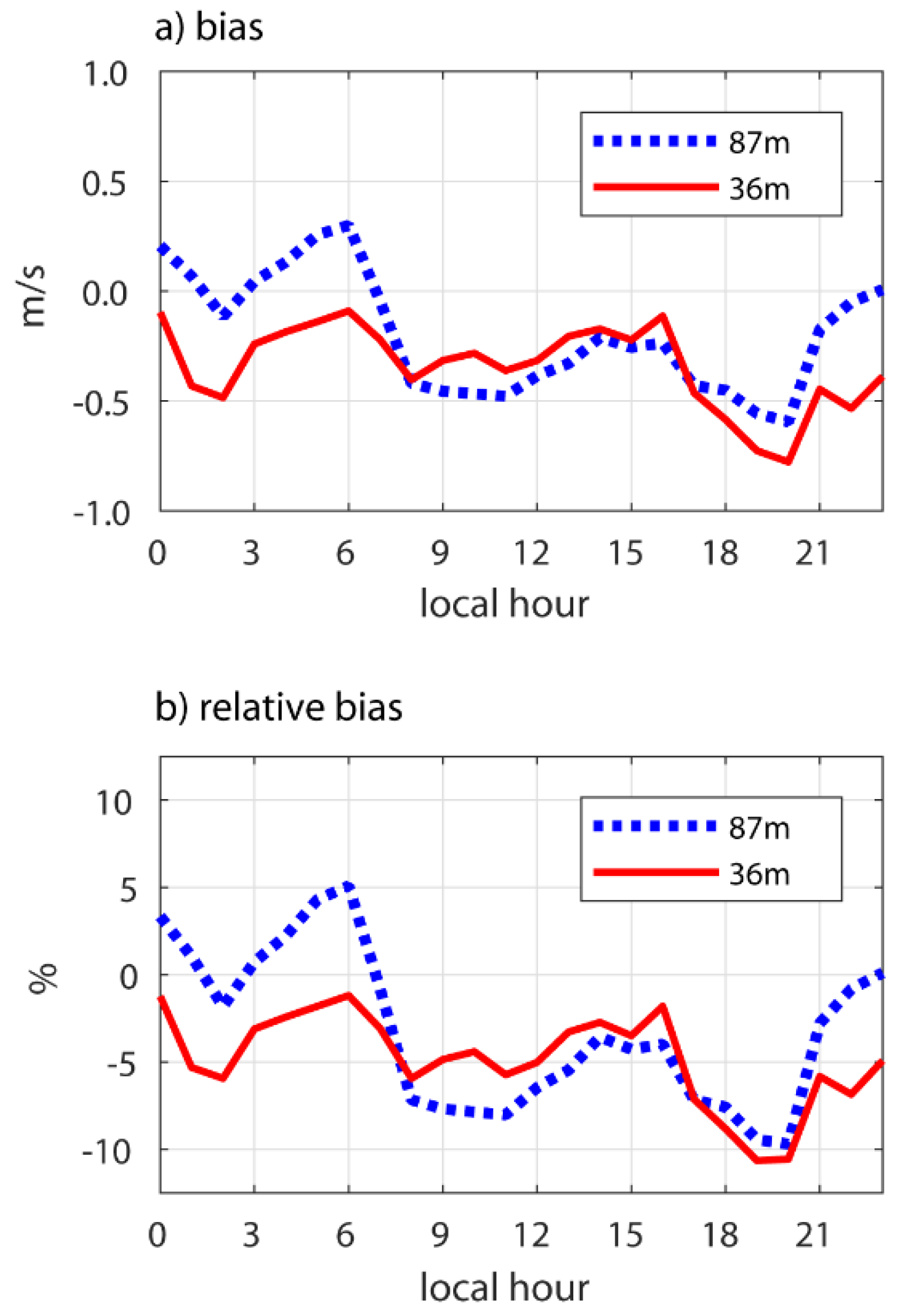
To evaluate the quality of the obtained pseudo-observations, we interpolated each component of the wind vector to the geographic location of VSt and the levels of 87 and 36 m above the ground, and then we computed the wind speed at these levels. Figure 4a shows the systematic error or bias of the two levels for each hour of the day. The bias is defined as the average of the wind estimate at a given level and hour minus the corresponding observed value over all the studied days:

$$b\equiv \overline{s_a}-\overline{s_{obs}}$$

(5)

where $s_a$ is the wind speed interpolated from the analysis to the location and level of each Vst sensor, and $s_{obs}$ is the correspondent measured wind speed. The overline represents the average over all the studied days. Figure 4b shows the relative bias, defined as the bias divided by the observed mean wind speed at the corresponding hour:

$$b_{rel}\equiv \frac{\overline{s_a}-\overline{s_{obs}}}{\overline{s_{obs}}}$$

(6)

At 87 m, the bias was moderate, generally smaller than 0.5 m/s, while relative bias was generally smaller than 5%. At 36 m, the bias and the relative bias were similarly moderate: the bias was generally smaller than 0.5 m/s, while the relative bias during some hours was slightly larger than that found at 87 m. Note that 87 m above the ground was similar to the elevation of the assimilated observations, while the 36-m elevation was significantly closer to the ground. The moderate systematic errors found at both elevations indicated that the data assimilation technique effectively combined the information from short-term WRF predictions and wind measurements. The wind measurements from the wind farms lacked information about elevations relatively close to the ground, e.g., at 36 m, while the WRF simulations did include this information since they considered several elevations within the first 100 m above the ground but had errors of their own. The assimilation process corrected these errors at the locations and elevations of the anemometers in the wind farms and also transmitted the effects of these gains to other regions and elevations. 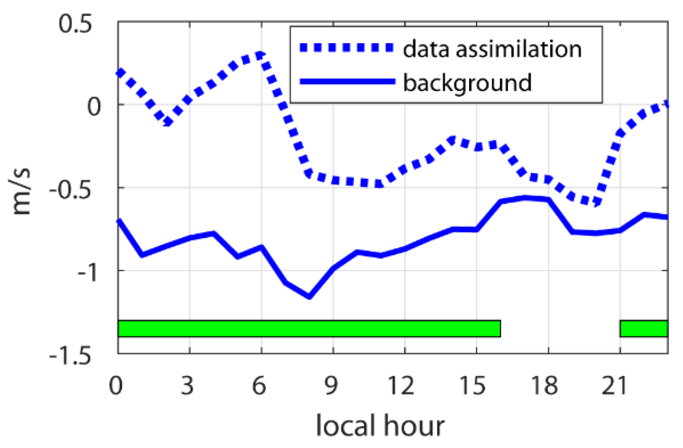The information that allowed these gains to spread was contained in the background error matrix B. To further illustrate this point, Figure 5 shows the bias of the background conditions 36 m above the ground at VSt and the bias resulting from the assimilation process (also included in Figure 4a). The background bias was larger for all hours. Since both biases were means of errors, it was possible to compute the significance of their difference with a two-tailed Student t-test [19]. It was found that these biases were different with a significance value lower than 0.05 for the local hours from 0:00 to 16:00, and from 21:00 to 23:00 (the hours with significant differences are indicated with a green bar in Figure 5).

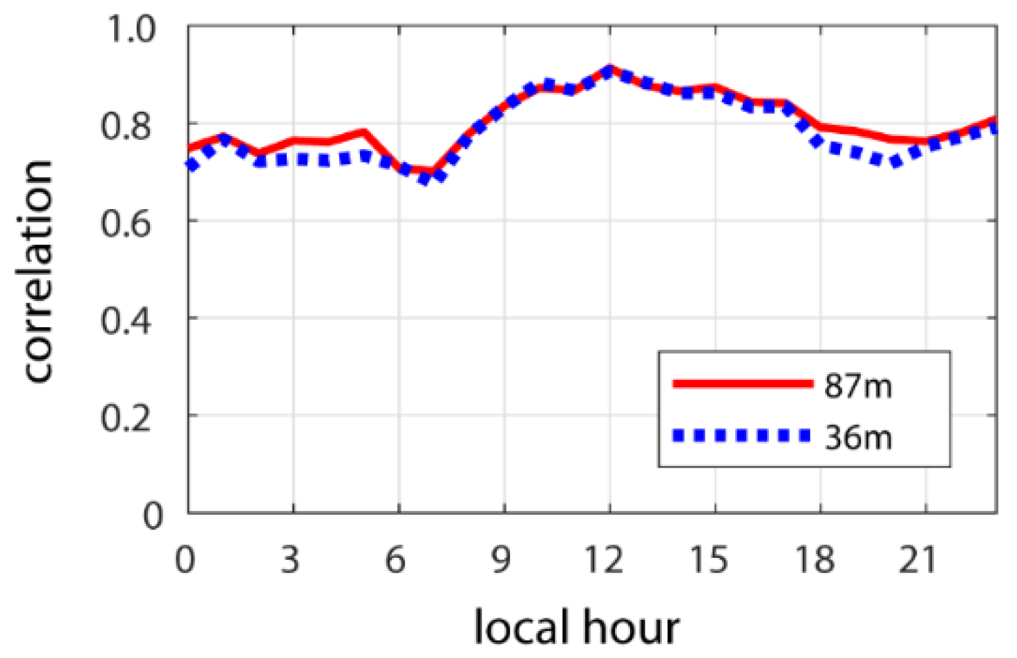
Next, we presented two statistical parameters related to accidental errors. Figure 6 shows the Pearson correlation of estimated versus observed wind speeds at the VSt station. At 87 m above the ground, there were correlations generally larger than 0.75 during the night hours, and generally larger than 0.80 during the day. At 36 m, the values were slightly smaller at nighttime and very similar during the day. 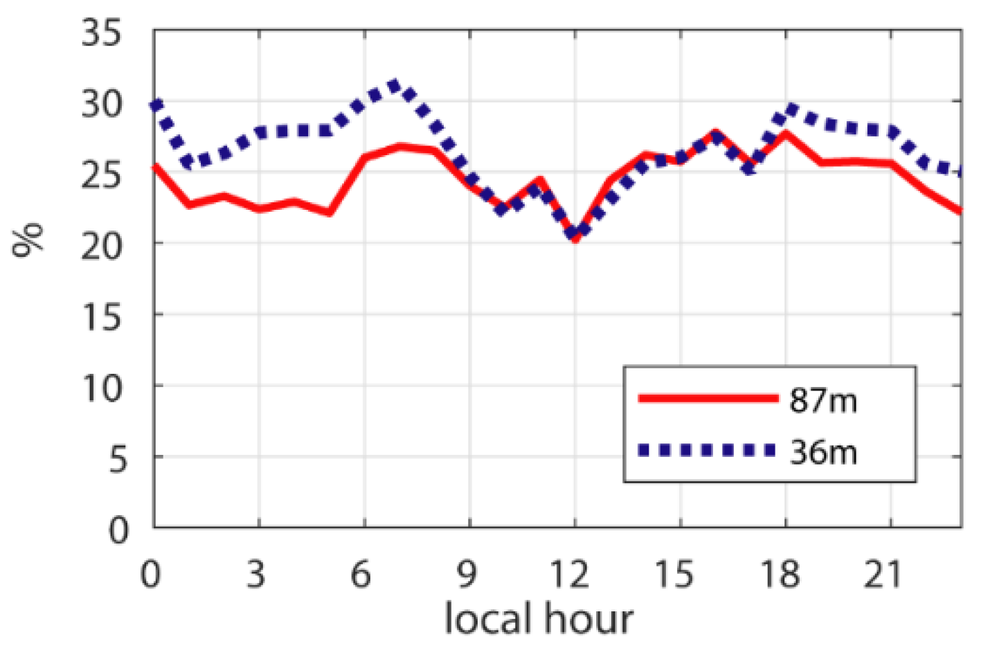Figure 7 shows the standard deviation of the error (estimated minus observed values) divided by the mean observed wind speed at each hour (RSTD). RSTD was approximately 25% for both elevations considered.

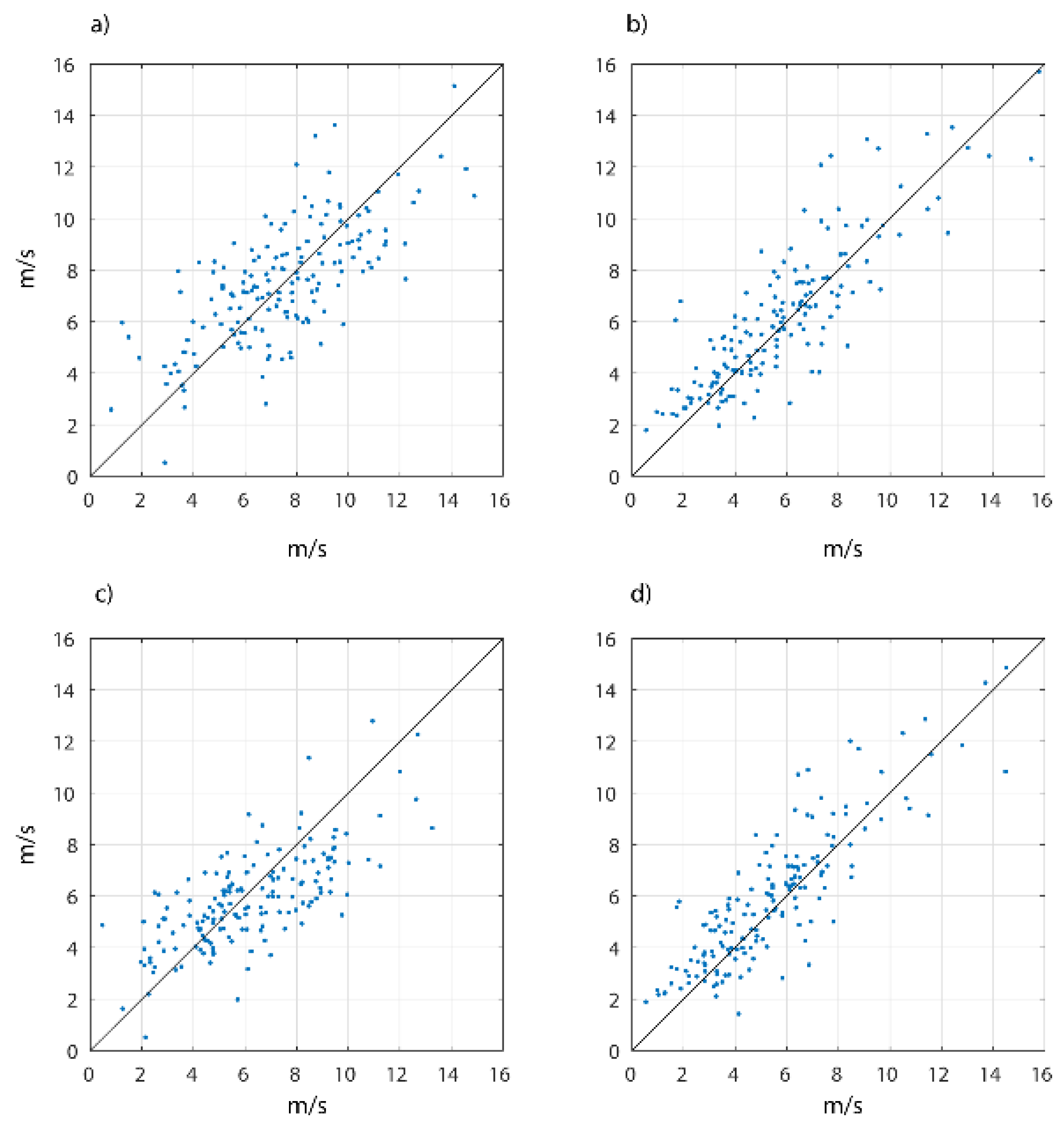
Figure 8 shows scatter plots of estimated versus observed wind speeds at 7:00 and 12:00 and 87 and 36 m above the ground. These hours were chosen because they represent the periods of the day with the relatively worst and best adjustments, as assessed in Figure 6 and Figure 7. Samples of assimilated values and the corresponding observed wind speed values, including those shown in Figure 8, made it possible to estimate probability distributions of the errors, such as empirical percentiles, from which confidence intervals for the wind speed estimates could be calculated.

5. Summary and Conclusions

This work assessed the quality of wind speed estimates in Uruguay obtained with the WRF-DA system, which was used to assimilate wind speed measurements 100 m above the ground at two wind farms. The quality of the estimates was assessed with an anemometric station placed between the wind farms, that measured wind speed at 87 and 36 m above the ground. The information to be assimilated from field measurements was minimal, not only because it included only two stations but also because it lacked records of other atmospheric variables that are related to wind, such as atmospheric pressure. It was interesting to assess the extent to which these minimum field measurements could generate useful interpolations and evaluate the quality of the wind estimates at elevations both similar and different to those of the assimilated records. The measurement station used to validate the wind speed assessments was placed between those used for the assimilation process, so the conclusions of the assessment are applicable only to regions between the two main stations.

Wind speed estimates showed a low systematic error at the verification station, generally below 0.5 m/s at both 87 and 36 m above the ground. A relative systematic error was generally less than 5% of the average speed. This result indicated that the data assimilation technique effectively combined information from field measurements and background conditions. The assimilated measurements did not include information from elevations as low as 36 m. The background conditions did contain information from these low elevations, but with systematic errors of their own. The assimilation technique managed to propagate the gain from the observations at 100 m above the ground in the wind farms to other regions and to lower elevations. The covariance matrix of the background condition error was essential to the propagation of these observational gains.

As for the total error, the correlation values between observed and estimated wind speed and the standard deviation of the total error of each estimate, generally about 1 m/s to 1.5 m/s, suggested that the obtained estimates could be of sufficient quality to be useful in various applications. Some examples of applications in which such estimates are valuable are the estimation of wind climatology within the range of the considered height levels, retrospective simulations of transport processes and dispersion of air pollutants, or real-time estimation of environmental conditions in which systems whose operation can be affected by the wind are being used. In any case, the effective use of pseudo-observations in a specific application requires the estimation of their confidence intervals, which are necessary both to assess whether the accuracy of pseudo-observations is acceptable for the application in question and to take into account the effects of the uncertainty of these data if they are used. The generation of databases of pseudo-retrospective observations, such as the one presented in this work, allows for the estimation of these confidence intervals.

For future studies, we are interested in quantifying the effects of including atmospheric pressure observations on the quality of the results. We are also interested in evaluating the effect of expanding the region in which observations are collected for the assimilation of data on the results of the hot start option.

Finally, we pointed out that the topography of the studied region is not completely flat but is relatively smooth. This can contribute to the quality of results obtained by assimilating a few observations in numerical simulations with relatively low resolution. In the case of regions with relatively complex topography, the numerical simulation may require finer spatial resolution to properly take into account the effects of topography on the wind field. The proper quantity and location of measurement stations should also be evaluated in each case.