A Topology Based Spatio-Temporal Map Algebra for Big Data Analysis

Abstract

Continental and global datasets based on earth observations or computational models challenge the existing map algebra approaches. The available datasets differ in their spatio-temporal extents and their spatio-temporal granularity, which makes it difficult to process them as time series data in map algebra expressions. To address this issue we introduce a new map algebra approach that is topology based. This topology based map algebra uses spatio-temporal topological operators (STTOP and STTCOP) to specify spatio-temporal operations between topological related map layers of different time-series data. We have implemented several topology based map algebra tools in the open source geoinformation system GRASS GIS and its open source cloud processing engine actinia. We demonstrate the application of our topology based map algebra by solving real world big data problems using a single algebraic expression. This included the massively parallel computation of the NDVI from a series of 100 Sentinel2A scenes organized as earth observation data cubes. The processing was performed and benchmarked on a many core computer setup and in a distributed container environment. The design of our topology based map algebra allows us to deploy it as a standardized service in the EU Horizon 2020 project openEO.

1. Introduction

Continental and global time series data from earth observation satellites [1,2,3] or computational simulations with arbitrary spatio-temporal granularities require very sophisticated tools for efficient analysis and processing. The NASA Landsat mission produces a large time series of earth observation data using different spectral bands that differ in their geographical locations, spatial resolution, spatial extents and their sensing time. The same is true for the ESA Copernicus mission, that includes a wide range of earth observation satellites. The publicly available NASA and ESA earth observation archives contain multiple petabytes of data, growing by several petabytes each year. There are several public global and continental climate datasets [4] available with high spatial- and temporal resolution.

A rapidly changing global environment, the global climate change, its continental and global effects on agriculture or natural hazards raise the requirement to analyse these large time series data and their relations to each other. A major challenge from the perspective of data analysis is how to process this kind of data altogether, handling the different spatio-temporal extents and their different spatio-temporal granularities.

In this research we develop a topology based map algebra to process large scale time series datasets with different spatio-temporal granularities and extents using algebraic expressions. We show how to apply topological algebraic expressions to Landsat8, Sentinel2A and climate time series data to compute vegetation indices and hydro-thermal coefficients. We demonstrate the big data analysis capabilities of the topology based algebra by computing the NDVI from 100 Sentinel2A scenes using the tools that we developed on a many core computer system and a distributed docker container environment. Our research is based on the spatio-temporal capabilities of the temporal enabled GRASS GIS [5]. It makes use of spatio-temporal topological features of the GRASS GIS Temporal Framework [6] to formulate algebraic expressions with spatio-temporal topological operators.

2. Related Work

The book [7] from Dana Tomlin introduced the concept of map algebra as a general language in geographical information systems (GIS) for analysis and processing of raster based geographic data with two dimensions. This data is mainly referenced as raster layers in GIS. By integrating time as the third dimension by [8,9] a new class of algebra was introduced into the GIS world. The new map algebra approach works on space-cubes, time-cubes and hyper-cubes that have two to three spatial- and one temporal dimension. Space-, time- and hyper-cubes have by definition equidistant spatial dimensions and require periodic time intervals that are equidistant. The computational spatial region must be equal for all layers in these cubes.

The map algebra approach of Dana Tomlin are available in many GIS applications. The GIS software systems GRASS GIS, ArcGIS and ERDAS Imagine integrate map algebra concepts. The Google Earth Engine [10] framework supports two different approaches to apply mathematical operations on images1. It is possible to use algebraic expressions with spatial, comparison and logical operators or nested functions on image objects. However, mathematical operations can not be applied on times-series data2 directly. The user must implement code to iterate over an image collection or map an algorithm to apply mathematical operations for each image in the collection.

2.1. GRASS GIS

We chose GRASS GIS to implement the topology based map algebra, because it is a full-featured, free and open source temporal geographical information system [5,6,11]. GRASS GIS has been used in numerous environmental scientific applications by [12,13,14,15,16]. A comprehensive overview of its application in environmental modelling is given in [17].

The temporal enabled GRASS GIS can efficiently manage, analyse and process continental- and global-scale time-series raster, 3D raster or vector data sets. Being free and open source allows users to modify it, which enabled us to integrate the topology based map algebra as a main feature.

Our topology based map algebra was implemented as three new modules in the temporal enabled GRASS GIS version 7 [5]. It utilises the GRASS GIS Temporal Framework [6], PyGRASS [18] and the GRASS GIS modules g.copy3, r.mapcalc4 and r3.mapcalc5.

2.2. Actinia

Actinia [19] is an open source REST API for scalable, distributed, high performance processing of geographical data that uses GRASS GIS for computational tasks. It provides a REST API to process satellite images, time series of satellite images, arbitrary raster data with geographical relations and vector data. We improved Actinia in context of this work to support massive parallel processing of topology based map algebra expressions in a distributed cloud environment. Actinia and GRASS GIS are software components of the EU Horizon 20206 openEO project [20], that is an open source interface between earth observation data infrastructures and front-end applications. Actinia is actively developed and deployed on different cloud platforms from cloud provides like Amazon, Google, Deutsche Telekom and others.

2.2.1. Time in GRASS GIS

The temporal enabled GRASS GIS uses the concept of linear, discrete time represented by time instances and time intervals. Time intervals and time instances represent the time stamps of map layers. Time intervals are left closed and right open. The end time is not part of the time interval but represents the start time of a potential successor. Time intervals can overlap or contain each other. The temporal model supports gaps and time instances. Time in GRASS GIS is described in detail in [5].

Time is measured using the Gregorian calender time, also called absolute time, conform to ISO 86017 and as relative time defined by an integer and a unit of type year, month, day, hour, minute or second. The smallest supported temporal granule is one second. The definition of absolute and relative time follows the temporal database concepts collected in [21].

2.2.2. Map Algebra in GRASS GIS

The GRASS GIS module r.mapcalc and r3.mapcalc implement a subset of the map algebra functionality described in [7,8,9], especially the local and focal algebraic methods. Zonal algebraic methods are performed by dedicated GRASS GIS modules like r.series, r.neighbors, r.univar, r3.univar, r.stats, r3.stats and several others.

With the integration of time in GRASS GIS by [5] the space-cube map algebra module r3.mapcalc was enabled to perform spatio-temporal operations on time-cubes using the existing map algebra syntax.

2.2.3. Data Cubes in GRASS GIS

A data cube is an aggregation concept from relational databases introduced by [22] that works on attribute data organized in a N-dimensional cube. We use the concept of earth observation data cubes, that organize earth observations like satellite images in a multi-dimensional cube. Dimensions are spatial and temporal coordinates, attributes are pixel values.

Space-time datasets (STDS) are the spatio-temporal data types in GRASS GIS to manage series of time-stamped map layers and were introduced in [5]. They can be interpreted as sparse data cubes with irregular time dimensions. There are three spatio-temporal GRASS GIS data types:

• Space-Time Raster Datasets (STRDS) that manage time series of raster map layers. These are sparse raster data cubes in which each time stamped slice stores only pixels from the area of interest in this slice, that can be different from any other slice and is a subset of the spatial extent of the whole data cube.
• Space-Time Raster 3D Datasets (STR3DS) that manage time series of 3D raster map layers. These are sparse voxel data cubes, using the same storage approach as the STRDS.
• Space-Time Vector Datasets (STVDS) that manage time series of vector map layers. STVDS can be interpreted as vector data cubes.

An arbitrary number of time-stamped map layers can be registered in a single space-time dataset. A single time-stamped map layer can be registered in several different space-time datasets at the same time. Space-time datasets have a dedicated temporal type. Therefore a STDS can have either absolute time or relative time. The same is true for time-stamped map layers.

STDS can contain map layers that have time intervals or time instances attached as time stamps. Intervals and instances of time can be mixed in a space-time dataset. The spatial extents and spatial resolutions of associated raster or 3D raster map layers in a STDS can be different. See [5,6] for more details.

2.3. Temporal Granularity and Topological Relations

A calendar has multiple granularities that can be described using a temporal hierarchy, see [23]. We use the temporal Gregorian calendar hierarchy of years, months, days, hours, minutes and seconds. A year is composed of 12 months, a month contains between 28 and 31 days, a day has 24 h, a hour has 60 min and one minute has 60 s. A glossary about temporal granularity is available in [24]. The temporal granularity is defined in the GRASS GIS Temporal Framework as the largest common divider of time intervals and gaps between intervals or instances from all time-stamped map layers that are collected in a space-time dataset (STDS). It supports space-time datasets that have complex temporal structures. 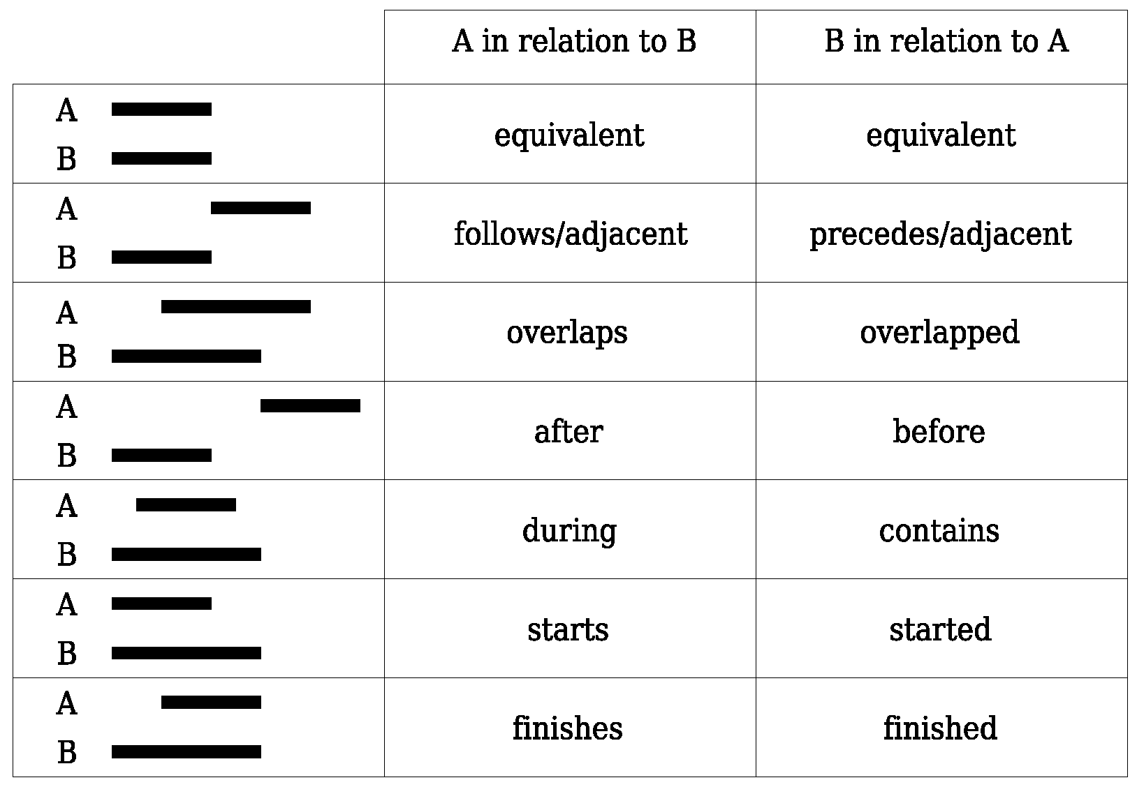See [6] for more details. Temporal relations between time-stamped map layers follow temporal interval logic defined by [25], see Figure 1.

The GRASS GIS Temporal Framework can compute topological relations between the spatial extents in two and three dimensions based on [26], see Figure 2. Spatial extents are represented as axis aligned bounding boxes.

2.4. Spatio-Temporal Operations

Spatio-temporal operations are based on the approaches implement in the GRASS GIS Temporal Framework by [6]. It provides boolean operations like intersection, union, disjoint union on time intervals and time instances. It support spatial boolean operations between spatial extents. As boolean operations, spatial intersection, spatial union and spatial disjoint union are available.

3. Topology Based Spatio-Temporal Map Algebra

We designed our topology based map algebra to perform two different tasks. The first task is the creation of subsets from space-time datasets based on algebraic expressions. That allows us to extract map layers from different space-time datasets based on their spatio-temporal topological relations. We implemented the dedicated GRASS GIS module t.select to perform such tasks. This module supports as input all STDS types that can also be mixed in a single expression. This algebraic approach is also part of the second task.

The second task is to perform spatio-temporal operations between STDS of the same type. We implemented this approach for STRDS and STR3DS as GRASS GIS modules t.rast.algebra and t.rast3d.algebra.

The syntax of the topology based map algebra is similar to the syntax of r.mapcalc [27]. The result of an algebraic operation is a new STDS. Two GRASS GIS modules r.mapcalc and r3.mapcalc are used to perform the spatial operations on raster layers, space- and time-cubes in our topology based map algebra.

A spatio-temporal expression of our topology based map algebra has the following form:

$$STDS=expression$$

A new space-time dataset is created by an expression that contains other space-time datasets, raster or 3D raster map layers, scalars, spatio-temporal operators as well as spatial and temporal functions.

An important feature of our topology based map algebra is the application of computational regions based on the spatial-extents of raster map layers that are involved in a single spatial operation. Hence, time-stamped raster map layers in a STRDS can have different spatial extents. This mode is activated by using the -s flag in the GRASS GIS algebra module t.rast.algebra. It assures that spatial operations that are applied to spatio-temporal related raster map layers are using the disjoint union of all spatial extents and the smallest raster cell size of all involved raster map layers for this operation.

3.1. The Spatio-Temporal Topological Operator STTOP

A core feature of our topology based map algebra is the spatio-temporal topological operator (STTOP). This operator defines what spatial and temporal operations should be performed between two entities. An expression involving the STTOP has always the following form:

$$leftentity\{STTOP\}rightentity$$

The spatio-temporal topology of an entity is arbitrary, it can contain components with equal, overlapping or including time stamps and spatial extents. The following entities are supported in an expression:

$$\begin{array}{cc}\hfill expression& :=STDS\{STTOP\}STDS\hfill \\ & :=STDS\{STTOP\}maplayer\hfill \\ & :=STDS\{STTOP\}scalar\hfill \\ & :=STDS\{STTOP\}expression\hfill \\ & :=expression\{STTOP\}STDS\hfill \\ & :=expression\{STTOP\}maplayer\hfill \\ & :=expression\{STTOP\}scalar\hfill \\ & :=expression\{STTOP\}expression\hfill \end{array}$$

Expressions can be nested. The result of an expression evaluation is an entity that always contains a series of time-stamped components of type map layer or scalar. The temporal topology is evaluated between the time-stamped components. Spatial topology evaluation is performed between time-stamped map layers.

A single map layer as well as a scalar can be defined as entity on the right side of the STTOP. In this case the single map layer or the scalar on the right side are applied to all map layers on the left side of the operator.

An operation between STDS A and B that result in a new STDS C can be expressed as:

$$C=A\{STTOP\}B$$

Operation between several STDS $A,B,C,D$ and E that result in a new STDS Z can be expressed as follows:

$$Z=A\{STTOP\}\left(\right(B\{STTOP\}C\{STTOP\}D)\{STTOP\}E)$$

Braces are used to specify non-default operator precedence’s, otherwise the operator evaluation is performed from the left to the right. Intermediate results are specified as $STDS$ $B^{*}$, $B^{**}$ and $B^{***}$ that represent a series of time-stamped components after expression evaluation. The evaluation and therefore the operator precedence of the expression above is shown below:

$$\begin{array}{cc}\hfill B^{*}& =B\{STTOP\}C\hfill \\ \hfill B^{**}& =B^{*}\{STTOP\}D\hfill \\ \hfill B^{***}& =B^{**}\{STTOP\}E\hfill \\ \hfill Z& =A\{STTOP\}{B}^{***}\hfill \end{array}$$

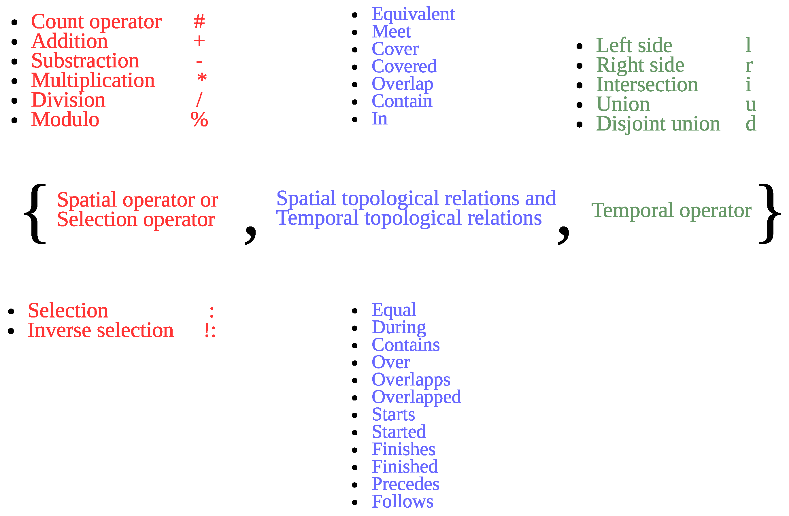
The STTOP can specify a selection operation or a spatial operation combined with spatio-temporal topological relations and temporal operators. It is shown in Figure 3 with all available sub-operators.

The STTOP is not commutative, the result of $A\{STTOP\}B$ may not be equal to $B\{STTOP\}A$.

3.1.1. Spatial Operators

Spatial operations are performed between raster map layers or between 3D raster map layers that have spatio-temporal topological relations to each other. A single scalar or series of time-stamped scalars can be used in a spatial operation as well. However, a series of time-stamped scalars is the result of an expression evaluation so that only single scalars can be specified directly in an expression.

Spatial operators are defined as the first sub-operators in the STTOP. If spatial operations are applied, new raster or 3D raster map layer will be created and registered in a new STRDS or STR3DS.

A special operator is the count operator that returns the number of time-stamped components on the right side of the operator that have adjacent temporal-topological relations to the time-stamped map layers on the left side of the operator.

All spatial operators are listed in

Table 1. Spatial operators and their precedence in the topology based map algebra.

Symbol	Description	Precedence
#	count	1
%	modulus	1
/	division	1
∗	multiplication	1
+	addition	2
−	subtraction	2

.

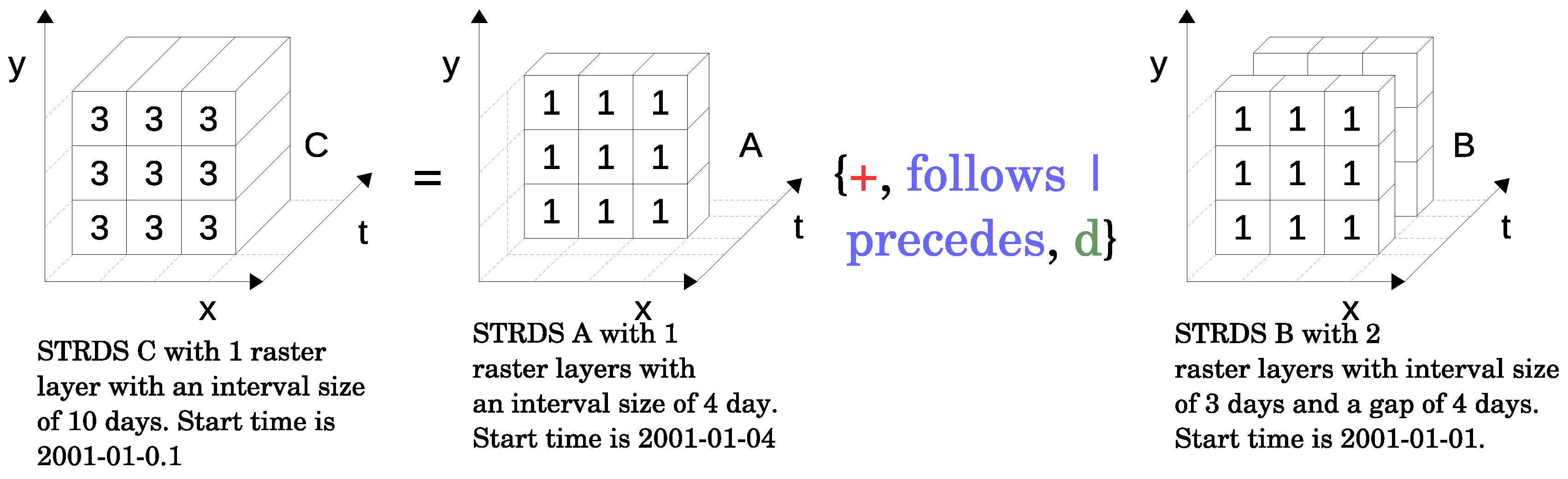
Spatial operators can be used directly in an expression, without the specification of temporal topological relations or operations. Then only time-stamped components with equal temporal topological relations are used in spatial operations. Equal spatial topological relations are not enforced because of the GRASS GIS computational region concept. For example, the creation of a new STRDS C that contains the sum of raster map layers from STRDS A and STRDS B that have equal time stamps, can be expressed as:

$$C=A+B$$

3.1.2. Temporal Selection Operators

Temporal selection operators were introduced to select and extract map layers of different STDS that have certain spatio-temporal topological relations to each other. This operator is defined as the first sub-operator in the STTOP. The selection operator does not create new map layers. It selects map layers based on their spatio-temporal topological relations and registers them in a new STDS. If the selection operation performs temporal operations, like temporal extent intersection, then the resulting map layers are copies of the original map layers and new time stamps, based on the temporal operations, are assigned. The original map layer must be copied, since GRASS GIS does not support multiple time stamps for single map layers. The type of the resulting STDS is defined by the type of the most left STDS in a selection expression. All supported selection operators are listed in

Table 2. Temporal selection operators and their precedence in the topology based map algebra.

Symbol	Description	Precedence
:	Selection Operator	1
$!:$	Inverse Selection Operator	1

. Examples for temporal selections are available in Appendix C.

3.1.3. Spatio-Temporal Topological Relations

Spatio-temporal topological relations are defined as the second sub-operators in the STTOP. Operations between two series of time-stamped components are based on their spatio-temporal topological relations to each other. Using topological relations is a convenient way to handle time series of components that have arbitrary spatio-temporal topologies. Spatio-temporal relations as shown in Figure 1 and Figure 2 are used to decide what operations should be performed between time-stamped components that can be map layers or scalars.

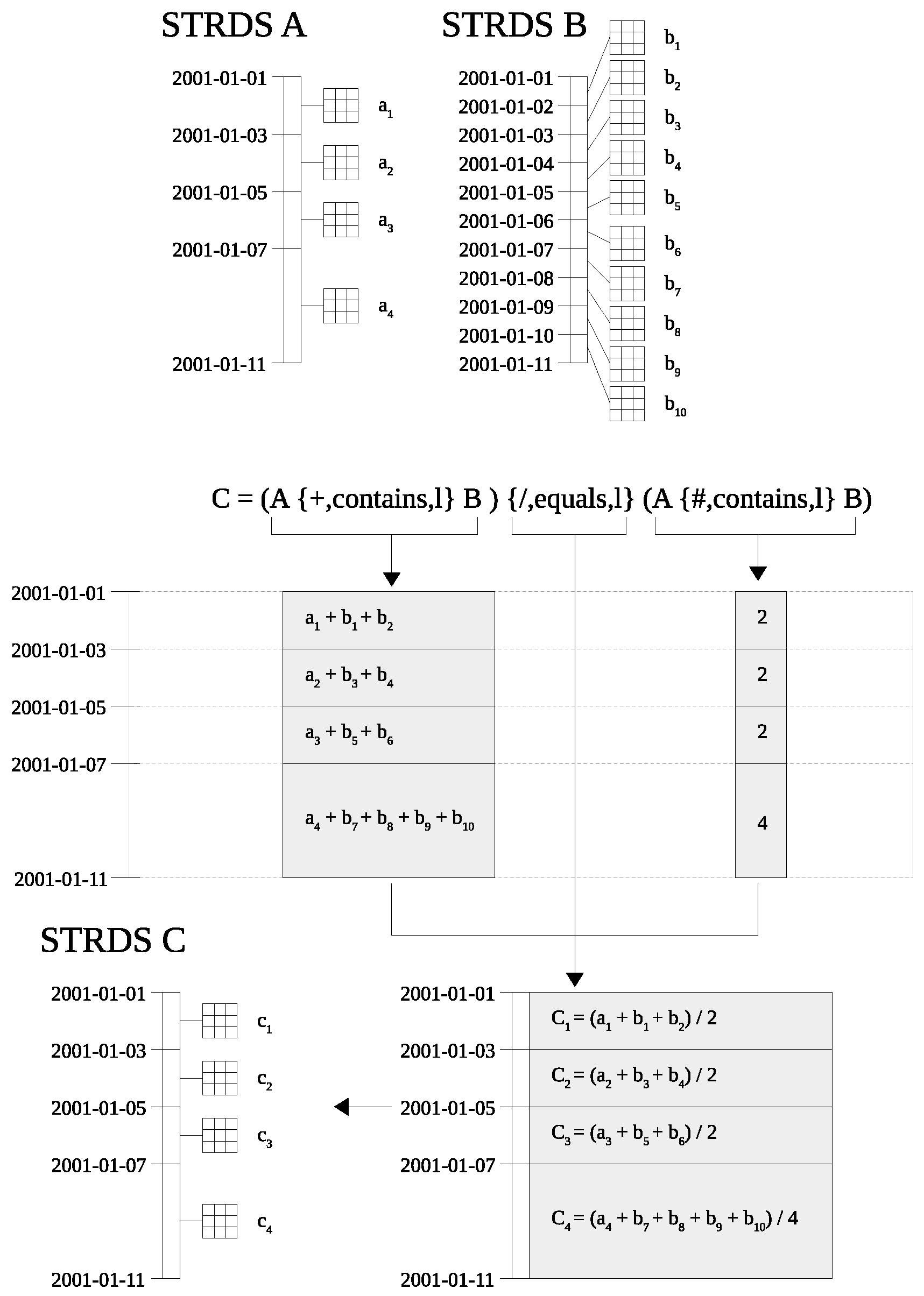
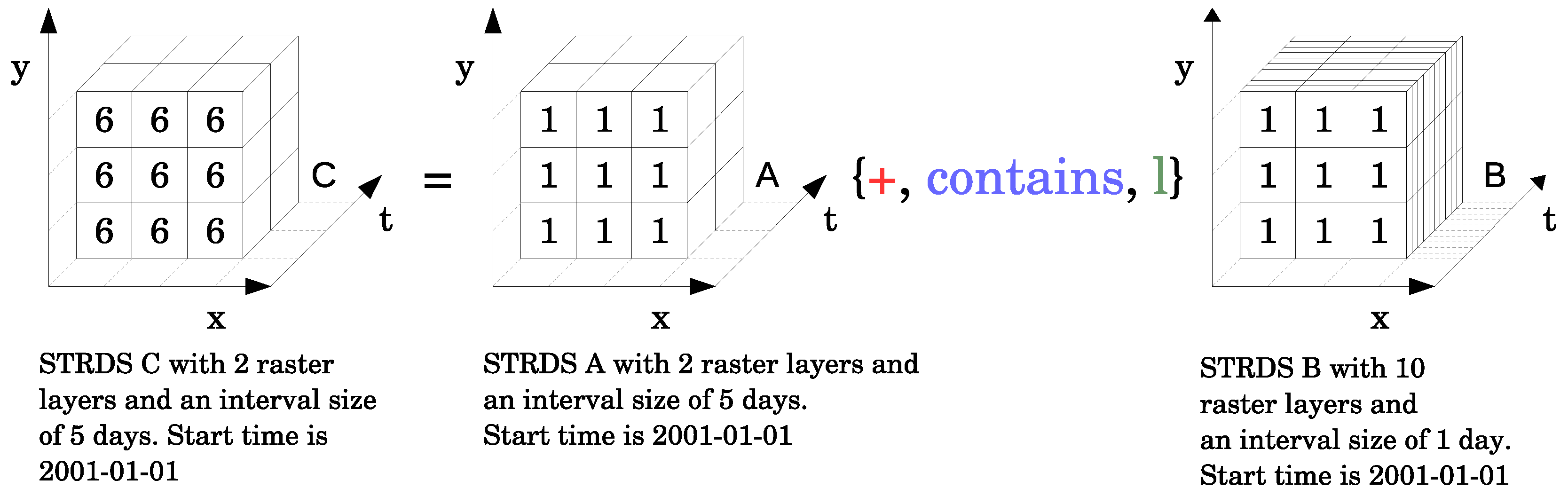
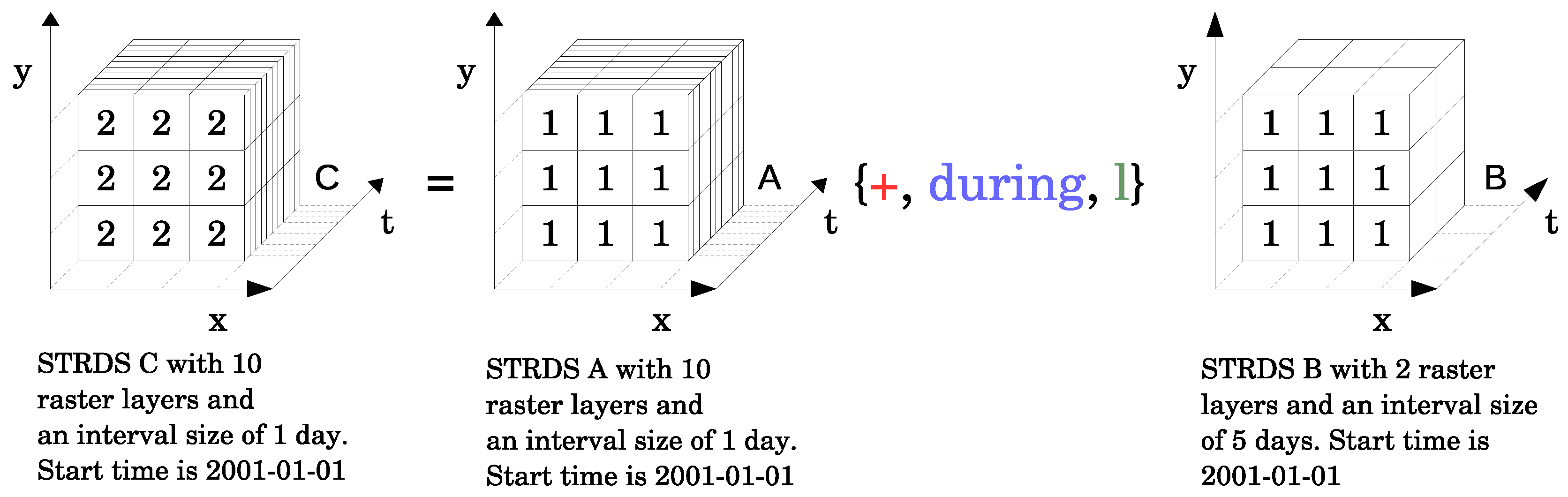
One or several topological relations can be specified as a single operator. Specifying several temporal topological relations will be interpreted using a boolean OR operation. The temporal topological relation is valid if one topological relation out of the specified list of relations is fulfilled. If several topological relations are fulfilled then a single map layer at the left side can be topologically related to many time-stamped components on the right side of the STTOP and vice verse. Specifying temporal or spatial topological relations can result in one to many relations between two series of time-stamped components. If one to many relations occur from the left side to right then an implicit aggregation approach is applied. A detailed example of implicit aggregation is described in Figure A1 in Appendix A.

Spatial and temporal topological relations can be combined in the second sub-operator. Temporal relations have OR relationships to each other. Spatial relations have also OR relationships to each other. However, temporal and spatial relationships are connected with an AND relation. This is important to distinct map layers that have equal time stamps but different spatial extents. If spatial and temporal topological relations are specified together as sub-operator, then one of the temporal and one of the spatial relationships must be fulfilled. The delimiter of a list of topological operators is the the logical OR |:

$$expression\{+,equals|during|equivalent,l\}expression$$

3.1.4. Temporal Operators

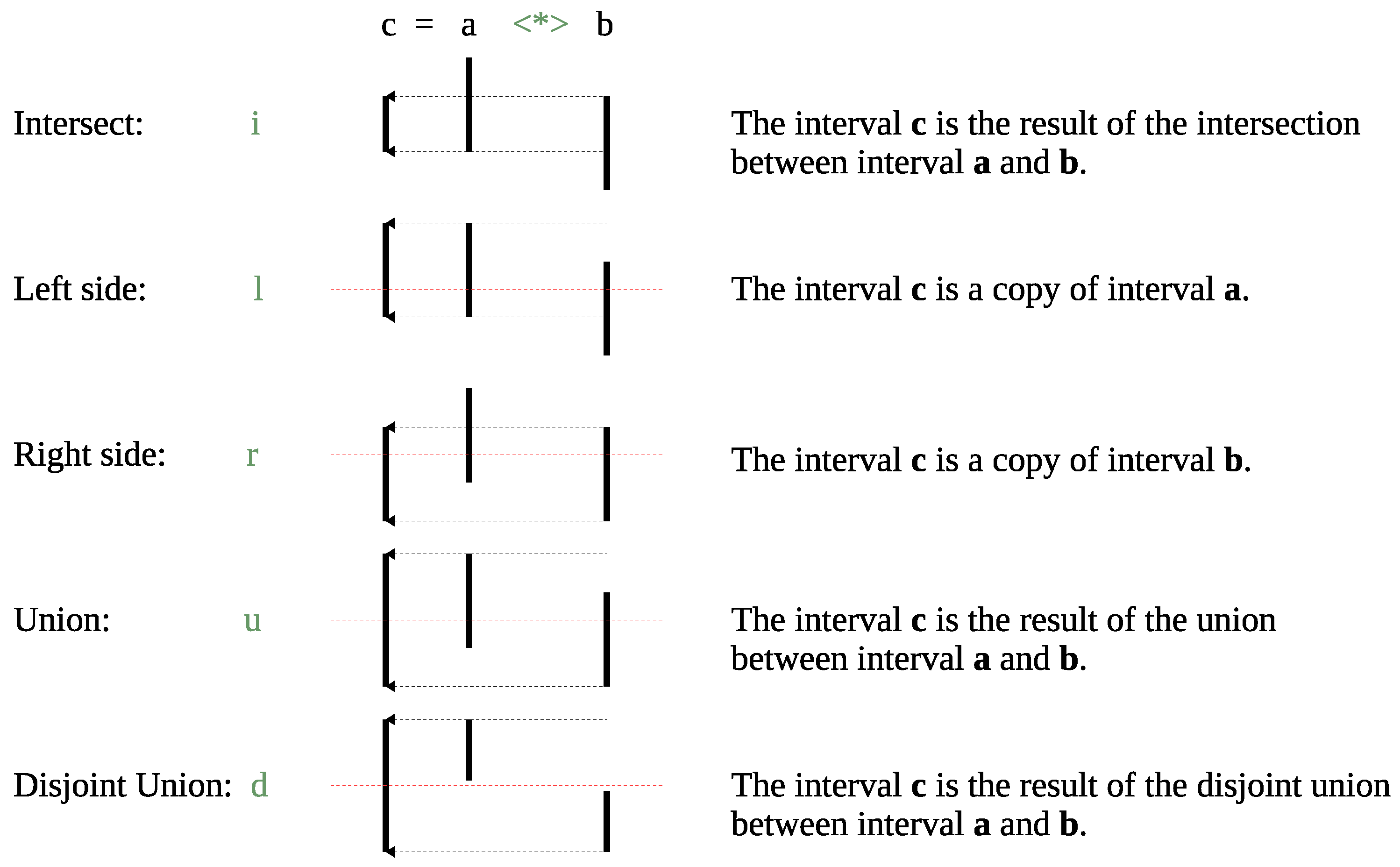
Temporal operators are located at the third position in the STTOP. They are performed between the temporal extents of two or more spatio-temporal related time-stamped components. The boolean temporal operations intersect, union and disjoint union are supported as well as decision operators left side and right side. The decision operators specifies if the time interval or time instance of a time-stamped map layer on the left side or of a time-stamped component on the right side of the STTOP should be used for the resulting time-stamped components of a selection or spatial operation. All supported temporal operations are shown in Figure 4.

3.2. Conditional Expressions

Conditional expression are required to formulate comparison and logical decision statements in our topology based map algebra. The syntax of conditional expressions is similar to [27] with the exception that topological relations must be specified. A conditional expression consists of an $if$ statement that specifies the comparison operations between STDS or time-stamped components and the $then$ and $else$ expressions. The result of a conditional expression is a series of time-stamped map layers.

$$\begin{array}{c}\hfill expression:=if(\{topologicalrelations\},\\ \hfill ifstatement,\\ \hfill thenexpression,\\ \hfill elseexpression)\end{array}$$

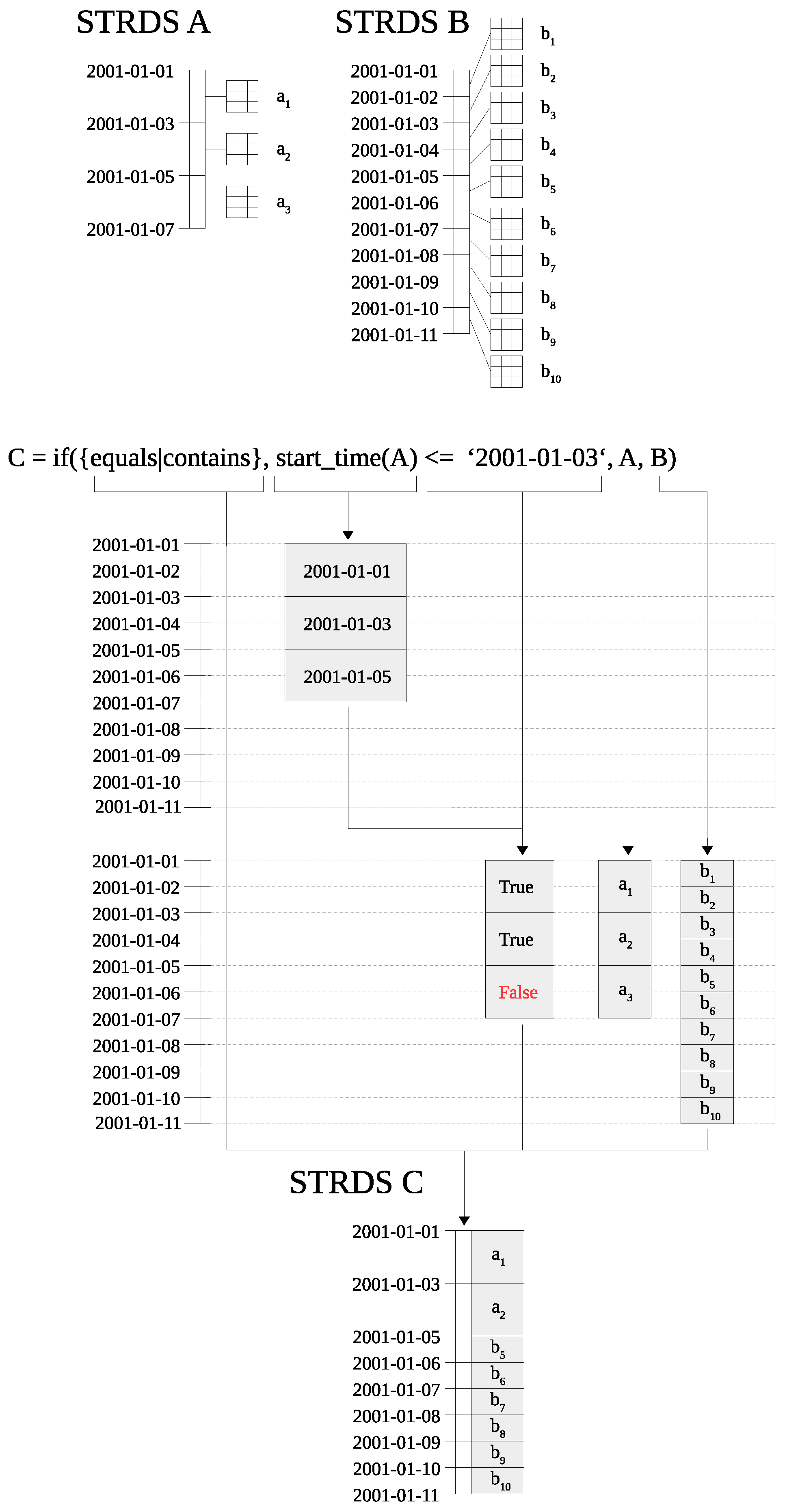
The Spatio-Temporal Topological Comparison Operator STTCOP

One key component of a conditional expression is the spatio-temporal topological comparison operator (STTCOP) that can only be specified in the $if$ statement. The spatio-temporal topological comparison operator must be used to specify comparison operations between time-stamped components like map layers, boolean values, scalars, date and time definitions. This operator expects a series of time-stamped components on the left and the right side. The result of the evaluation of a STTCOP is a series of time-stamped components. A single component can be of type map layer, scalar, date, datetime or boolean. Boolean, date and datetime component types are used in comparison operations. They cannot be used in spatial operations. The result of the evaluation of an $if$ statement is either a list of time-stamped boolean values or a list of spatial comparison operations. Topological relations defined before the $if$, $then$, $else$ expressions and time-stamped boolean values resulting from the evaluation of the $if$ statement are used to select the spatial operations performed in the $then$ or $else$ expression. Spatial operations of the $then$ expressions are performed if time-stamped boolean values are true and have a valid topological relation to the resulting map layers in the then expression. 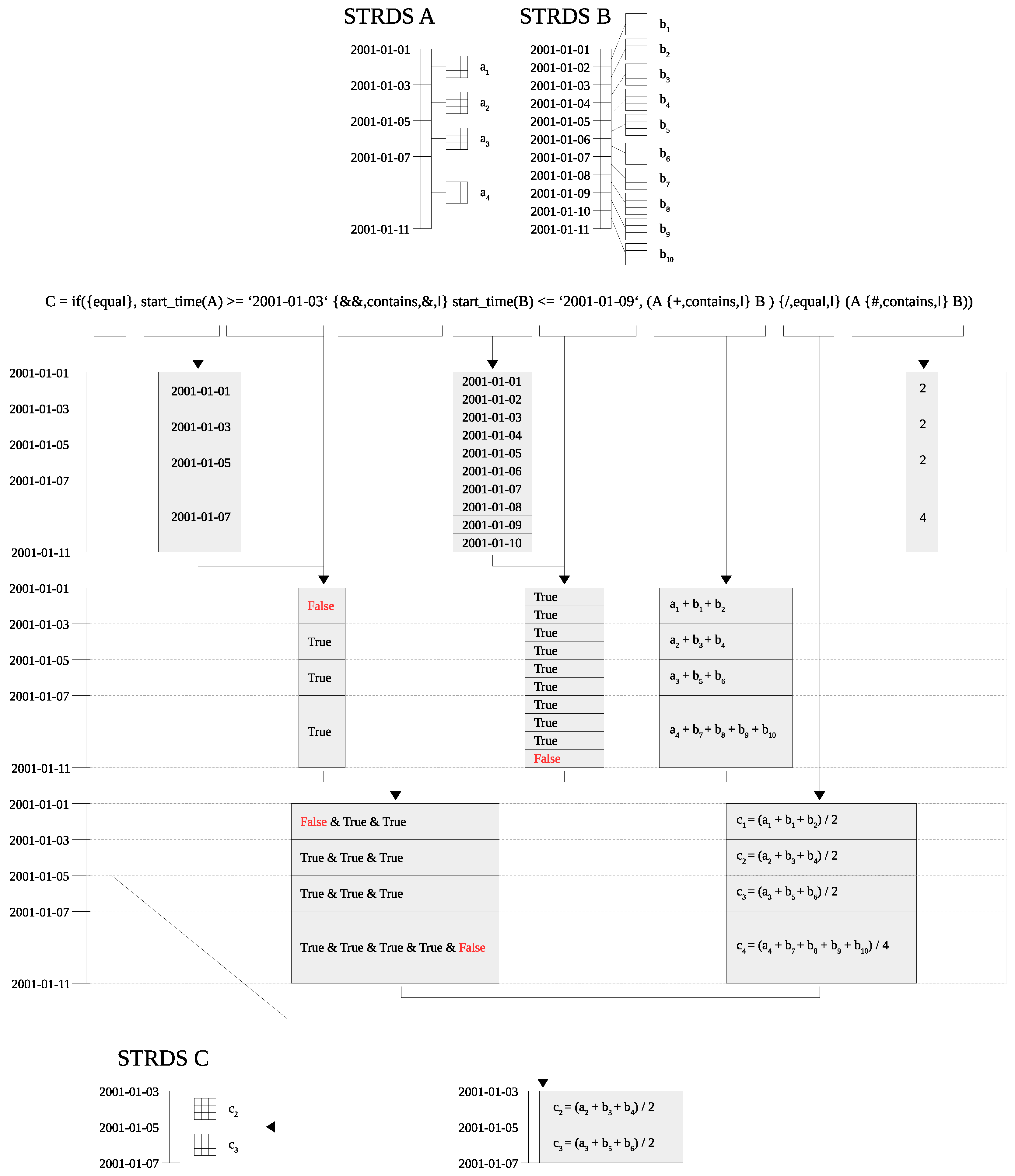Spatial operations in the else expressions are performed if no topological relation to the $if$ statement exists or if they are false. This is demonstrated in Figure A2 and Figure A3 in Appendix A.

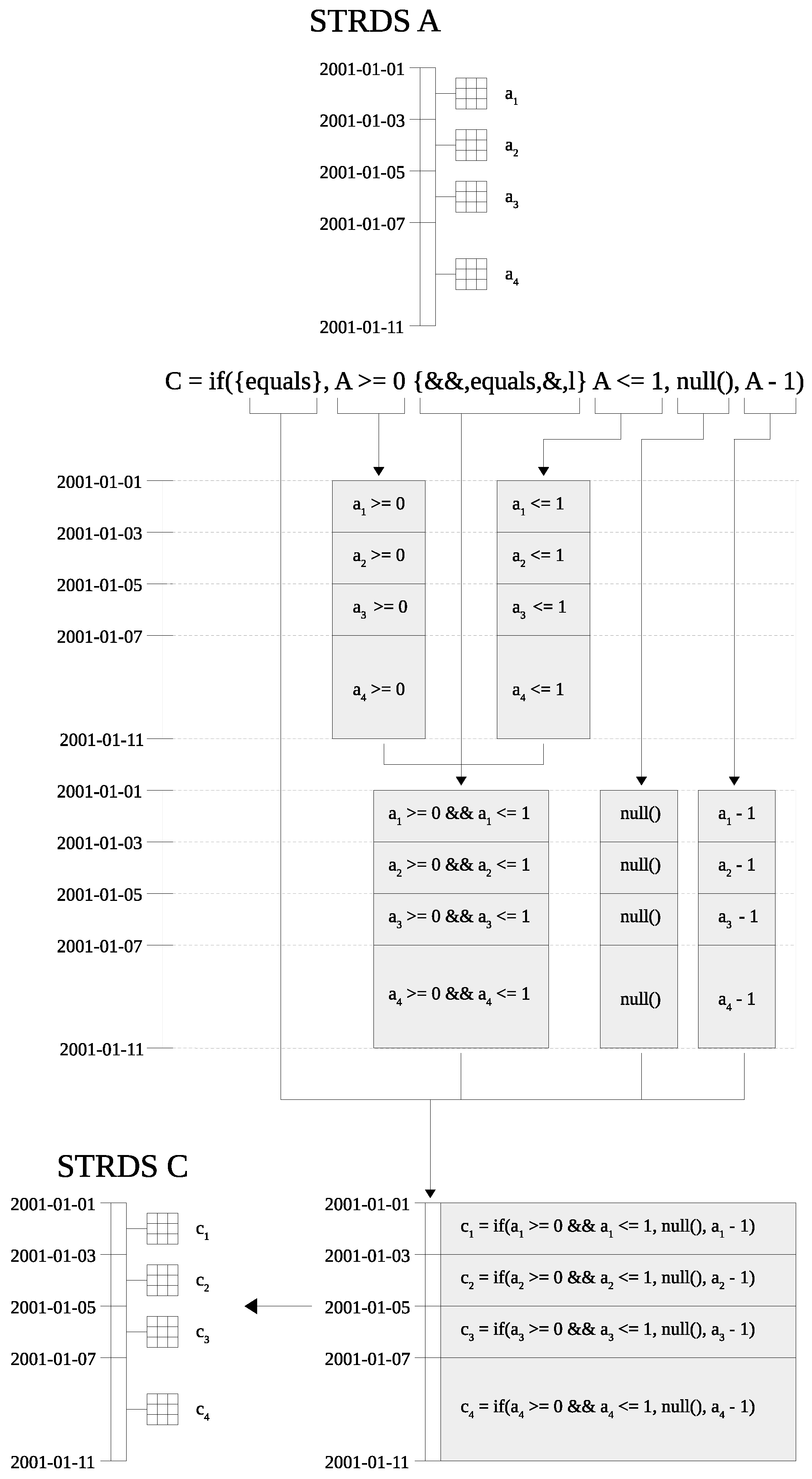
Spatial comparison operations are handled differently. They are applied to $then$ and $else$ expressions, if topological relations exist. Spatial comparison operations are then integrated in the resulting spatial operations. This is visualised in Figure A4 in Appendix A.

The STTCOP is not commutative, the result of $A\{STTOP\}B$ may not be equal to $B\{STTOP\}A$.

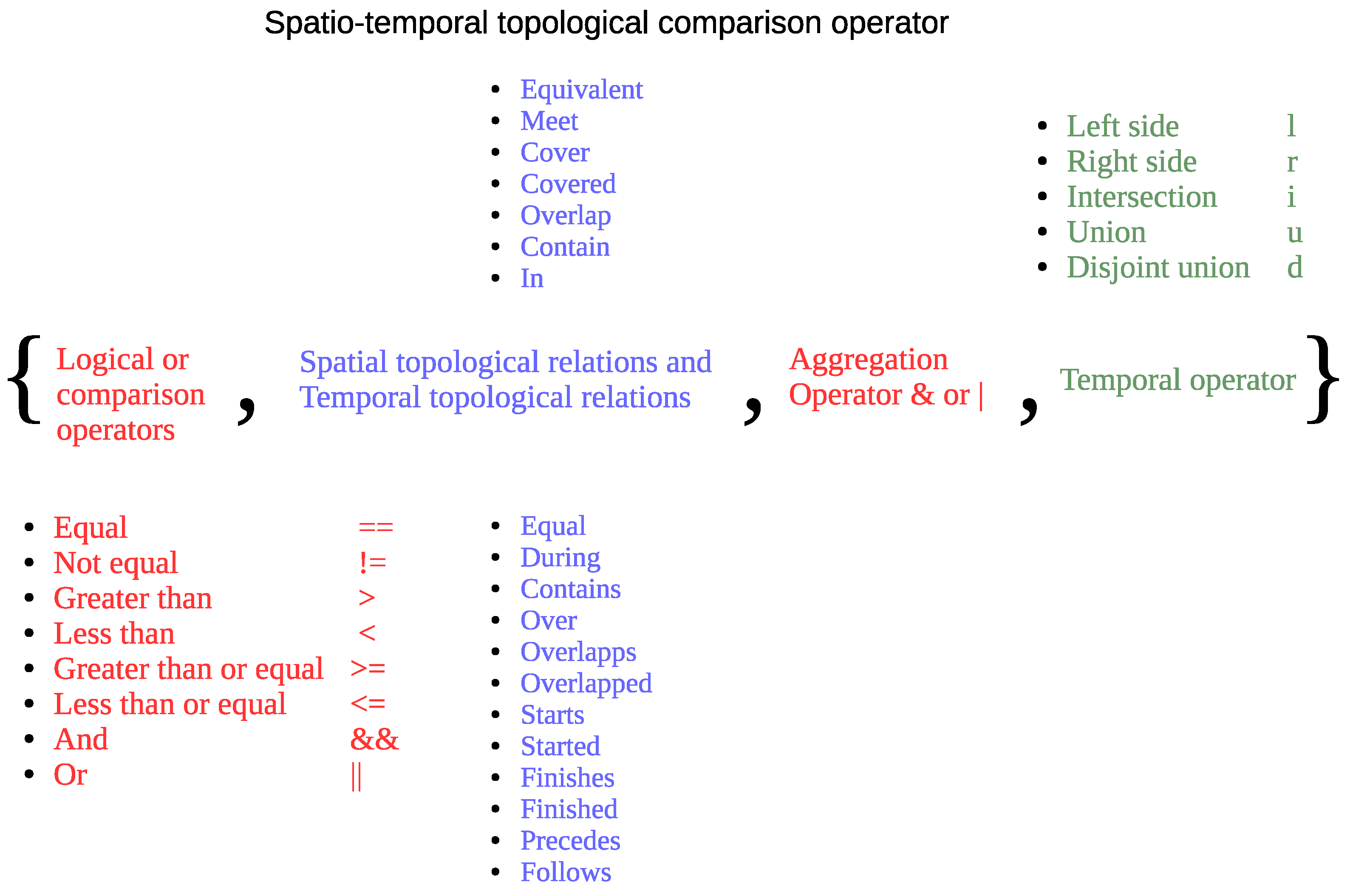
The STTCOP is described in Figure 5 with all available sub-operators. The STTCOP is build upon 4 sub-operators:

• The comparison operator;
• The spatio-temporal topological operator;
• The aggregation operator;
• The temporal operator.

The spatio-temporal topological operator and the temporal operator are similar to the STTOP. Specific for the STTCOP are the comparison, boolean and aggregation operators. The comparison and boolean operators are shown in

Table 3. Comparison and boolean operators of the STTCOP.

Symbol	Description	Precedence
$==$	equal	1
$!=$	not equal	1
>	greater than	1
$>=$	greater than or equal	1
<	less than	1
$<=$	less than or equal	1
$\&\&$	Boolean and	2
$\left|\right|$	Boolean or	2

. The aggregation operator is specified using the boolean AND & and OR | symbols. The cause of existence of these operators is the requirement to decide what kind of logical operation should be performed in a one to many relationship. If a time interval on the left side contains multiple time intervals with boolean values from the right side, the question arises how these values should be aggregated in a boolean operation? The aggregation operator describes the logical operations that should be performed between all boolean values on the right side of the STTCOP. An example of this operation is demonstrated in Figure A2.

The STTCOP can be simplified in the same way as the STTOP. Boolean and comparison operators can be used without specifying topological relations and temporal operations, if only equal temporal topological relationships are required. For example:

$$\{\&\&,equals,\&,l\}\to \&\&$$

$$\{>=,equals,l\}\to >=$$

3.3. Spatio-Temporal Functions

We implemented several spatio-temporal functions that include the following functionalities:

• Temporal buffering of time instances and time intervals;
• Temporal topological operation like shifting and snapping of time intervals;
• Mathematical functions like $log\left(\right)$, $sin\left(\right)$, $sqrt\left(\right)$, $null\left(\right)$ and many more;
• Date- and time functions like $start\_time\left(\right)$, $start\_year\left(\right)$, $start\_doy\left(\right)$ and many more;
• Special functions to use different spatio-temporal datatypes in a single expression like $map\left(\right)$ and $tmap\left(\right)$.

A complete list of spatio-temporal functions is available in Appendix B.

3.4. Neighbourhood Operations

The topology based map algebra supports neighbourhood operations based on indices. The syntax is similar to [27] with the difference that the temporal dimension was added. STRDS neighbourhood operations can be temporal $A[t]$ or spatio-temporal $A[t,x,y]$. The temporal index is based on a nearest neighbour approach rather then temporal topological relations like precedes or follows. This has the advantage that neighbourhood operations can also be performed on raster map layers that have time intervals or time instances and no adjacent temporal topological relations to their temporal neighbours. The difference between raster and 3D raster algebra is, that the 3D raster algebra is based on space time 3D raster datasets and a four dimensional neighbourhood operator $[t,x,y,z]$. Several examples are available in Appendix C.

3.5. Temporal Granularity Algebra Approach

The granularity mode in our topology based map algebra was introduced to handle topological well aligned STDS in a convenient way. In granularity mode all spatio-temporal operators in our topology based map algebra imply equal temporal topological relations between time-stamped map layers.

The GRASS GIS Temporal Framework provides methods to compute the temporal granularity of space time datasets with valid temporal topology based on the Gregorian calendar hierarchy [6]. It can determine if the granularity has the unit years, months, days, hours, minutes or seconds. Different space time datasets may have different temporal granularities. To perform spatio-temporal operations between them, one must know what their common temporal granularity is. Hence, the GRASS GIS Temporal Framework was extended to compute the common temporal granularity of series of time-stamped map layer, or STDS and to re-sample them by the common granularity.

For example, we assume that space time dataset A has a temporal granularity of one month. Space time dataset B has a granularity of 7 days. Their temporal extent starts at 1 January 2001 and ends 1 January 2002. We assume that the time-stamped map layers of A and B have the same interval size as the granularity. There are no temporal gaps between the time-stamped map layers. The common temporal granularity between A and B is one day. To perform spatio-temporal operations between the space time datasets A and B, we need to re-sample them to a common granularity of one day. This re-sampling operation will always be performed temporally. The re-sampling operation will result in the intermediate space time datasets $A^{*}$ and $B^{*}$. This operation is performed on the fly in memory, based on the temporal metadata and will not affect the original space time datasets. Hence, between 28 and 31 in memory map objects of $A^{*}$ with a daily interval size will point to the same physical map layer, dependent on the actual month. For space time dataset $B^{*}$ seven in memory map objects will point to the same physically map layer. This step assures that temporal topological relations between space time dataset $A^{*}$ and $B^{*}$ are reduced to equal, after, before, precede and follow. Therefore the STTOP and the STTCOP are simplified to spatial, selection and comparison operators.

This approach simplifies the handling of time with temporal or spatio-temporal operators. However, resulting space time dataset may have many more time-stamped map layers than the original space time datasets with plenty of redundant spatial and temporal information. It can not handle space time datasets with invalid temporal topology. However, the GRASS GIS Temporal Framework provides convenient functionality to compute valid temporal topology and to perform temporal aggregation of space time raster datasets.

4. Solving Real World Problems

4.1. Landsat NDVI Computation

The spatial operator allows us to apply the normalised difference vegetation index (NDVI) formula to a series of satellite images. An important requirement is that the satellite images are spatio-temporal distinctive from each other. This is the case for Landsat scenes, all bands of a single scenes have equal spatio-temporal extents that are distinct from any other Landsat scenes. We assume that the near infrared channel raster layers of several Landsat scenes are stored in STRDS $Landsat8\_NIR$. The red channel raster layers are stored in STRDS $Landsat8\_RED$. The NDVI computation for a time series of several Landsat scenes can now be formulated as a simple mathematical expression:

$$NDVI=(Landsat8\_NIR-Landsat8\_RED)/(Landsat8\_NIR+Landsat8\_RED)$$

The resulting algebraic expression applied with the command line tool t.rast.algebra to run in parallel on 8 dedicated CPU cores looks as follows:

t.rast.algebra
    basename=ndvi nprocs=8
    expr=“NDVI=(Landsat8_NIR - Landsat8_RED) /
               (Landsat8_NIR + Landsat8_RED)”
		

4.2. Sentinel2A NDVI Computation

The simple NDVI formula for Landsat time series can not be applied to Sentinel2A scenes, since different Sentinel2A scenes have different spatial extent but sometimes equal time stamps. They are not spatio-temporal distinctive. The expression must be extended with the spatio-topological relation equivalent to solve this issue, so that only scenes with equal spatio-temporal extents are used for the computation. We compute the normalised difference vegetation index (NDVI) for our dataset that consists of 100 Sentinel2A scenes from Germany using bands 4 and 8. We selected Sentinel2A scenes that were produced between 13 February 2017 and 6 July 2017. In addition we applied a filter to select only scenes that have an areal size greater then 5000 km² and cloud cover lower than 2%. The resulting dataset contained 200 time-stamped raster map layers organised in two STRDS ($S2A\_B08$, $S2A\_B04$) with a total size of 43 GB. We applied temporal and spatial topological relations to differentiate between time-stamped map layers with equal time stamps but different spatial extents.

The command to compute the NDVI on 8 dedicated CPU cores is:

t.rast.algebra
    basename=ndvi -s nprocs=8
    expr=“NDVI=(S2A_B08{-,equal|equivalent,l}S2A_B04)
                       {/,equal|equivalent,l} \
			   (S2A_B08{+,equal|equivalent,l}S2A_B04)”
		

We made use of the -s flag in t.rast.algebra to assure that the computational region is derived from the spatio-temporal related raster map layers that are involved in a spatial operation.

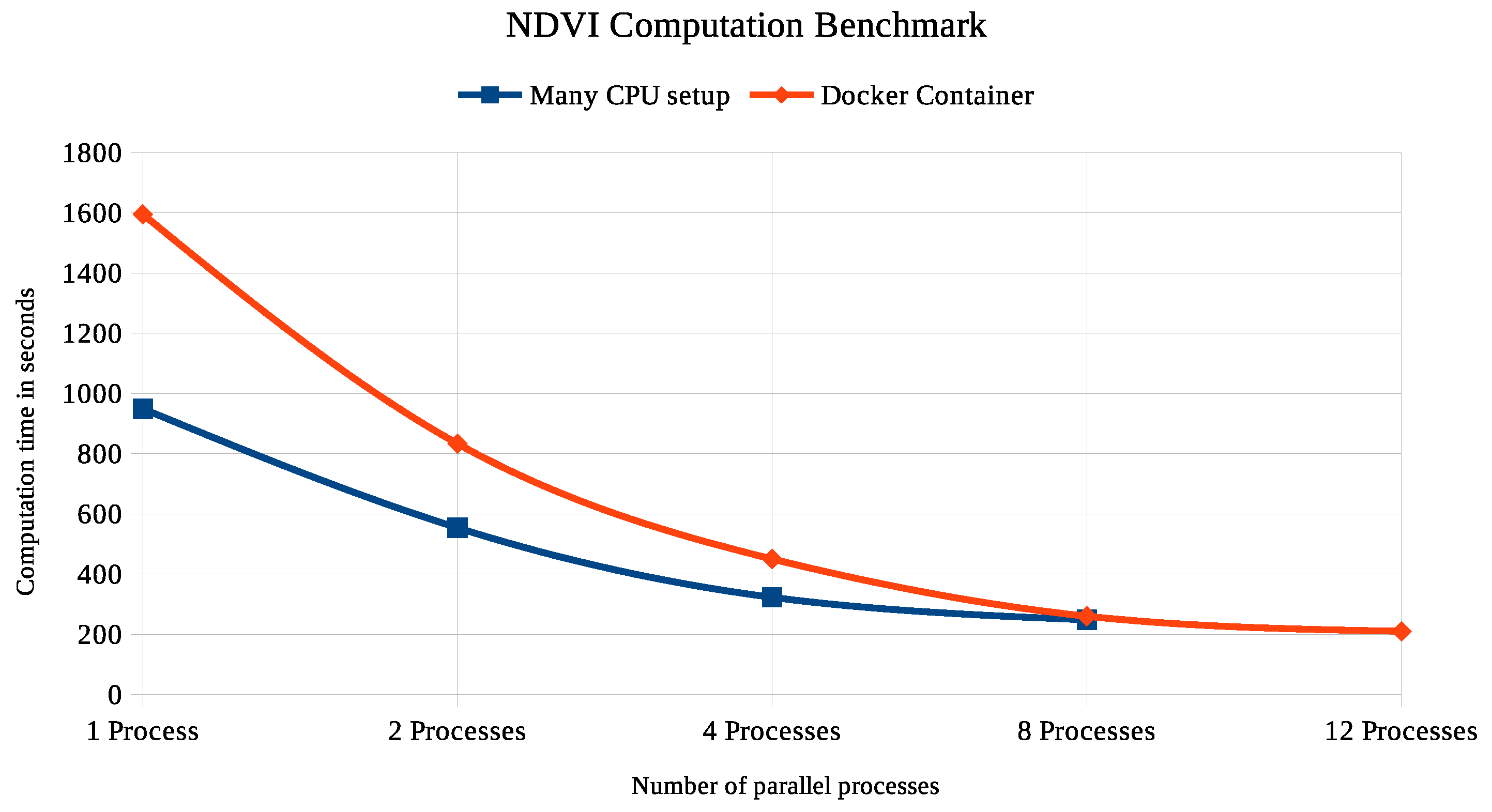
The GRASS GIS REST processing engine actinia was used to compute the same algebraic expression with a deployment of 12 docker container. The dedicated program actinia-algebra8 was implemented, to distribute the map algebra expressions generated by t.rast.algebra to all 12 container and to collect the result in a new STRDS. In Figure 6 is the process time shown to compute the NDVI from 100 Sentinel2A scenes using up to 8 CPU’s on a many core setup and up to 12 parallel processes on a docker container deployment.

4.3. Hydrothermal Coefficient Computation

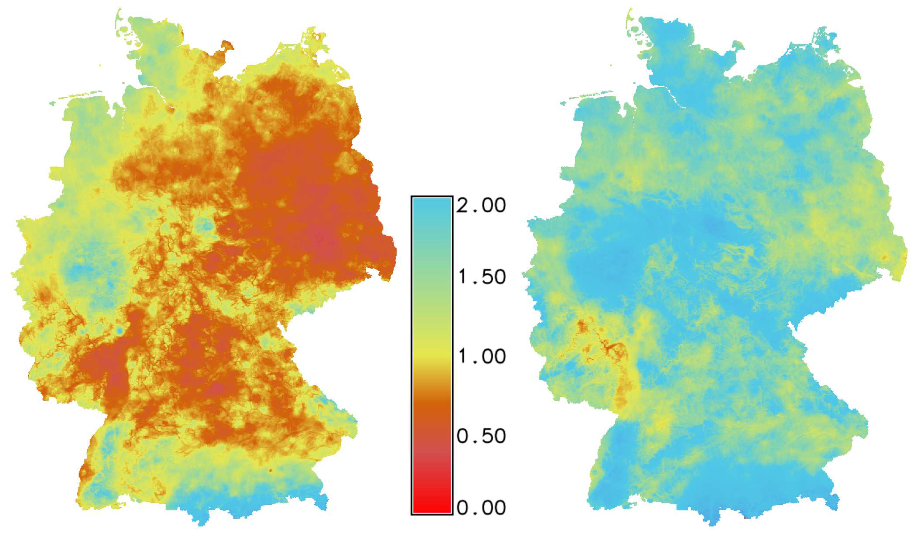
The hydrothermal coefficient is a simple measure for agricultural drought and is commonly used in eastern Europe for monitoring meteorological conditions. The index is based on daily temperature and precipitation values and is sensitive to dry conditions specifically in the temperate climate zone. It is calculated as the relation of the accumulated precipitation values to the temperature sum above a baseline temperature threshold value of 10 for annual periods. The mathematical formulae is:

$$HTC=\frac{\sum P_{(T>{10}^{\circ }C)}}{\sum T_{(T>{10}^{\circ }C)}·0.1}$$

The index can be formulated by using the implicit aggregation feature of the spatio-temporal algebra for different temporal granularities in combination with a conditional statement for the threshold temperature. Therefore an STRDS with zeros and annual granularity has to be created as mask for which the daily meteorological STRDS are aggregated.

The algebraic expression for the hydrothermal coefficient can be formulated as:

t.rast.algebra
  basename=htc nprocs=8
  expr=“HTC = (D {+,contains,l} if(T >=  10.0, P, 0.0)) /
              (D {+,contains,l} if(T >=  10.0, T / 10.0, 0.0))”

and is applied with the command line tool t.rast.algebra to run in parallel on 8 dedicated CPU cores, whereby three different STRDS are utilized:

• T := STRDS of daily temperatures,
• P := STRDS of daily precipitation
• D := STRDS of annual mask with 0 as pixel value

The result is shown in Figure 7. The index values range between 0 and 2, whereas zero values indicating intensive drought conditions and values above 1 represent a more humid year.

5. Discussion and Conclusions

We designed and implemented a new map algebra based on spatio-temporal topological relations. The syntax of the topology based map algebra was derived from the GRASS GIS map algebra module r.mapcalc. We extended the map algebra syntax by introducing a new spatio-temporal topological operator (STTOP) and a spatio-temporal comparison operator (STTCOP). Our topology based map algebra can therefore be easier understood by users, that are familiar with the syntax of existing map algebra implementations.

Our topology based map algebra allows selection operations as well as spatio-temporal operations on space-time datasets (STDS) based on spatio-temporal topological relations of the time-stamped map layers that are registered in the STDS. The selection part of our topology based map algebra works with all spatio-temporal datatypes that are available in GRASS GIS: STVDS, STRDS and STR3DS. Spatio-temporal operations can only be applied to STRDS and STR3DS. However, that means that our topology based map algebra works with 3 and 4 dimensions. The GRASS GIS space-time raster and 3D raster datasets can be interpreted as sparse data cubes with arbitrary time dimension. Hence, our topology based map algebra is designed to processes earth observation data cubes.

Spatial topological relations are based on the spatial extents of time-stamped map layers. Temporal topological relations are based on the temporal extents of time-stamped map layers. Spatio-temporal operations and topological relations must be specified as STTOP and STTCOP. In addition, useful spatial and temporal functions are available to modify STDS and to specify single maps and STDS of different types in a single expression. This is the first map algebra approach that allows the mixing of different datatypes in a single expression.

The STTOP and STTCOP are very powerful but its applications needs careful planning and can be very complex in nested expressions. The user must be aware of the temporal and spatial dimensions and the temporal topology of the STDS that are used in an expression. The usage of temporal and spatial topological relations must be carefully thought out to compute the required results.

The introduction of topological relations between time-stamped map layers in spatio-temporal operations leads to one-to-many relations between map layers. To address this issue we implemented the concept of implicit aggregation in case one-to-many relationships occur in the expression evaluation.

Both operators STTOP and STTCOP can be simplified in case the temporal topological relations between map layers are only equal, precedes and follows. Then simplified STTOP spatial operators and STTCOP comparison operators can be specified. This leads to less complex expressions and simplifies the application of our topology based map algebra.

We introduced the granularity mode in our topology based map algebra to simplify the handling of datasets with complex temporal topologies. In this mode all STDS that are specified in the algebraic expression will be temporally re-sampled to the greatest common temporal granularity. All time-stamped map layers will have the same temporal topology. Only equals, precedes and follows temporal topological relations are possible. Therefore, in granularity mode, all STTOP’s and STTCOP’s can be simplified to use only spatial and comparison operators in an expression.

Our topology based map algebra is not limited to a fixed computational region. The time-stamped map layers can have different spatial extents and spatial granularities. GRASS GIS will re-sample all raster and 3D raster maps on the fly based on nearest neighbour inter- or extrapolation. The algebra supports the definition of spatial relationships, so that only spatially related map layers are used for spatial operations. Our algebra supports the creation of computational regions based on the spatial extents of spatio-temporal-topologically related time-stamped map layers that are involved in a single spatial operation. This allows the application of algebraic expressions to time series of globally scattered satellite images without the need to create a computational region that includes the disjoint union of all spatial-extents of the time-stamped map layers that are used in the expressions. We demonstrated this in our NDVI computation of Sentinel2A satellite images example.

The implementation of our algebra is based on the GRASS GIS Temporal Framework. This framework provides many functionalities that were directly used in our algebraic approach. One functionality we would like to discuss is the ability to compute virtual space-time datasets (vSTDS) that can be used in other spatio-temporal operations in case of nested expressions. Each sub-expression is transformed in a vSTDS that consists of virtual map layers, that are defined by their spatio-temporal extents and an r.mapcalc operation. This functionality allowed us to implement lazy execution of the algebraic expressions. Hence, the full analysis of a topology based map algebraic expression eventually results in a list of independent r.mapcalc expressions and time stamping operations that can be executed massively parallel. This allows us to distribute the computation of any algebraic expression over many cores on a single computer, or over several computer nodes in a cluster or cloud environment. The many core approach was successfully demonstrated in the Sentinel2A NDVI computation example that includes a benchmark of processing time dependent on the number of used CPU cores.

The actinia processing engine was used to demonstrate the massively parallel processing of a single algebraic expression in a distributed container deployment. Hence, our topology based algebra can be deployed as a web service to perform complex algebraic computations on massive datasets. The actinia geo-processing engine allows to deploy GRASS GIS and other geo-tool based algorithms as REST service where earth observation data is physically stored. It runs on Telekom-, Google- and Amazon-Cloud platforms that provide direct access to earth observation data from satellites as Sentinel2A, Sentinel2B and Landsat. GRASS GIS and actinia are software components of the openEO initiative that provides standardized connections to and between earth observation providers. Two authors of this work are actively involved in the openEO initiative which opens the possibility to deploy our topology based map algebra as a standardized openEO processing service.