Agro-Climatic Data by County: A Spatially and Temporally Consistent U.S. Dataset for Agricultural Yields, Weather and Soils

Abstract

Agro-climatic data by county (ACDC) is designed to provide the major agro-climatic variables from publicly available spatial data sources to diverse end-users. ACDC provides USDA NASS annual (1981–2015) crop yields for corn, soybeans, upland cotton and winter wheat by county. Customizable growing degree days for 1 °C intervals between −60 °C and +60 °C, and total precipitation for two different crop growing seasons from the PRISM weather data are included. Soil characteristic data from USDA-NRCS gSSURGO are also provided for each county in the 48 contiguous US states. All weather and soil data are processed to include only data for land being used for non-forestry agricultural uses based on the USGS NLCD land cover/land use data. This paper explains the numerical and geo-computational methods and data generating processes employed to create ACDC from the original data sources. Essential considerations for data management and use are discussed, including the use of the agricultural mask, spatial aggregation and disaggregation, and the computational requirements for working with the raw data sources.

Dataset: The csv formatted ACDC datasets are freely downloadable from http://dx.doi.org/10.4231/R72F7KK2. Documentation and support for end-users include a user’s manual, as well as a set of default maps and weighting schemes. The current version is v.1.0.0 for 1981–2015. The ACDC dataset will be updated regularly following source dataset updates. All datasets are built using R 3.3.2 or above.

Dataset License: CC-BY

1. Introduction

Agriculture is one of the most impacted economic sectors studied in the context of climate variability and change [1,2]. The primary question about the relationship between agriculture and climate/weather (hereafter, agro-climatic relation) has been posed as: how will agricultural output change as a result of climate change or increased weather variability? These agro-climatic relations can be represented conceptually using a general functional form as:

$$Y=f\left(H,P,S,E,X\right),$$

(1)

where $Y$ is agricultural output, $H$ is heat (or temperature) exposure, $P$ is precipitation, $S$ is soil characteristics, E is other climate (environmental) factors, and $X$ is non-environmental socio-economic variables. In the literature, agricultural output is measured as crop yields [3,4], crop acreages [5], and agricultural land values [6]. As [7] pointed out, these outputs are used in agro-climatic models and assessments to provide insights into climate change and adaptation, food security, policy evaluation, development of decision-support tools for industry, farmers and policy makers, resource use and efficiency, yield gap analysis, and more.

Rapid recent technological improvements in high-resolution satellite imagery data (for simplicity, raster data1) have contributed to an increase in such agro-climatic research [8]. Publicly and freely available raster data have been widely employed to study the agro-climatic functional relationship described through two particularly popular research frameworks: regression-based analysis [9,10], and process-based models [11,12]. The current research aims to help a broader base of research and decision-support communities access these geo-spatial data products. Prospective users of these raster data often encounter several difficulties. Widely-used raster data sources are built on a fine grid-size (for example, 10 or 30 meter-resolution), and thus, their data size generally requires high-performance computing capability and time-consuming operations to extract the desired variables. Furthermore, while these data are freely available from government data repositories, specialized data users are assumed to know the methods and have the computational resources to acquire and manage the raw data from original raster data using GIS techniques or other data generating processes. The author of one of the most widely-cited agro-climatic studies, Wolfram Schlenker, alluded to the methodological and apparent technical difficulty in his blog:

“A funny thing about that paper [9]: many reference it, and often claim that they are using techniques that follow that paper… people have done similar things that seem inspired by that paper, but not quite the same. Either our explication was too ambiguous or people don’t have the patience to fully carry out the technique, so they take shortcuts.” (G-FEED, 1/10/2015)

2

The technical issues and obstacles are not limited to researchers. Many disciplines, as well as sophisticated decision-makers and practitioners, are not adept enough at data handling and processing to utilize the full array of agro-climatic data available today.

The Agro-climatic Data by County (ACDC) data set is developed to make disparate data from different sources, in different data formats, and on different spatial scales available to end-users of county-level agro-climatic data for analysis, decision-support or research. The ACDC provides the most widely-used variables extracted from high-resolution gridded data sources to end-users of agro-climatic variables who are not equipped to process large geo-spatial datasets from multiple publicly available sources that are provided in different data formats and spatial scales. In the current version (v.1.0.0), annual county-level crop yield data from the United States Department of Agriculture’s (USDA) National Agricultural Statistics Service (NASS) for 1981–2015 are provided for corn, soybeans, upland cotton and winter wheat, and customizable growing degree days (GDDs) and cumulative precipitation for two groups of months (March–August and April–October) to capture different growing season periods for the included crops from the PRISM (Parameter-Elevation Relationship on Independent Slopes Model) weather data. Other spatial weather data sources are available and will continue to be produced, but the PRISM is used for ACDC because it continues to be widely used in peer-reviewed literature and, in particular, in the authors’ own discipline of applied economics. Selected soil characteristic data processed from the USDA Natural Resource Conservation Service’s (NRCS) gSSURGO (Gridded Soil Survey Geographic database) are also included for each county in the data set. All weather and soil data are processed only for non-forestry agricultural land uses based on the US Geological Survey (USGS) NLCD (National Land Cover Database) land cover data. The weather and soils data included in ACDC only correspond to the land actually being used for agricultural production. This paper explains the numerical and geo-computational methods and data generating processes employed to construct the ACDC using R.

The present paper is organized as follows. In Section 2, the spatiotemporal extent and outline of ACDC are described. In Section 3, the numerical and geo-computational methodologies used in ACDC generation are explained in detail. In Section 4, the issues of constructing county-level data from a raster database relevant to ACDC are discussed. In the final section, concluding remarks and the expected schedule for future updates to the ACDC are provided.

2. ACDC Dataset Outline

The raster data available for agro-climatic studies come from different sources, in different data formats, and are aggregated at different spatial scales. In this section, the ACDC dataset contents are described to explain how the data are assembled in common spatial and temporal units.

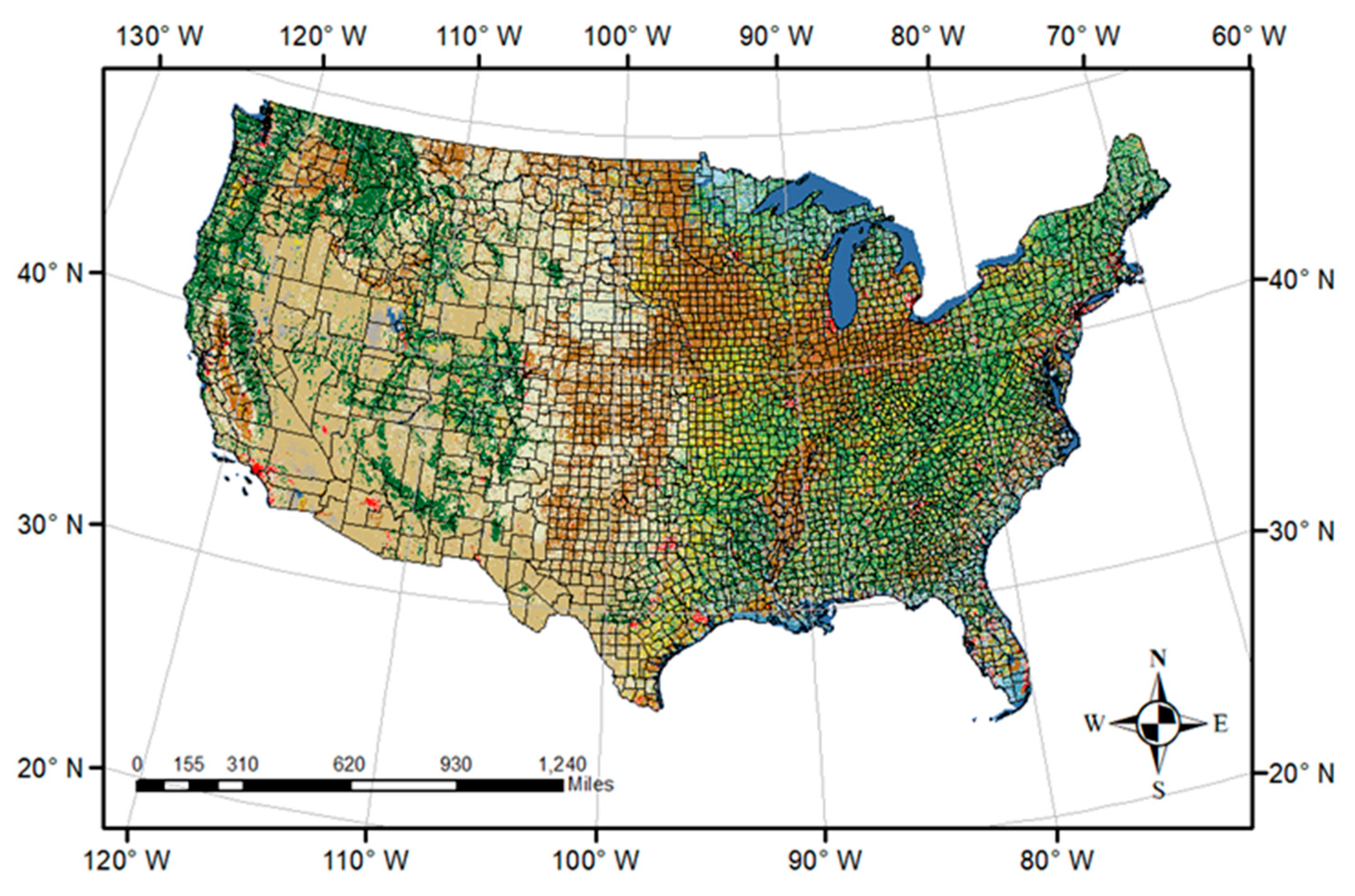
2.1. The Spatial and Temporal Extent of ACDC

The most widely available and used agricultural output ($Y$ in Equation (1)) data are county-level crop yield and acreage variables available from USDA-NASS. The administrative boundaries of counties are from the 2012 Agricultural Census (most recent year available) County map, which contains the geographical boundaries for USDA-NASS data collection. The original county boundary shapefiles for the whole US are available from: https://www.agcensus.usda.gov/Publications/2012/Online_Resources/Ag_Atlas_Maps/ (Accessed on 28 February 2017). Based on these shapefiles, the ACDC includes 3070 counties over the 48 contiguous US States shown in Figure 1 that overlap the 2011 NLCD map.

The downloadable ACDC package contains the shapefiles of the counties shown in Figure 1 in the zip file named <cntymap.zip>. This zip file includes three shapefile components: cntymap.shp, cntymap.dbf, and cntymap.shx.3

Every county boundary includes multiple land uses/covers, such as forest, cities, or water in addition to agricultural fields. Because the ACDC is only concerned with agricultural outputs, all variables included in the ACDC are based on land areas with agricultural fields only. To exclude non-agricultural land covers, the agricultural mask used in the ACDC is based on the NLCD maps available for each four-year period at the time of ACDC data processing. The method employed to apply the agricultural mask is discussed in the following section in detail. To manage various coordinate reference systems from raster data sources, ACDC used the default projection of the NLCD to maintain the accuracy of variables. ACDC users are recommended to use the NLCD projection when working with the geo-spatial data provided.4

Because heat exposure and precipitation data in ACDC are dependent upon daily weather fluctuations, the temporal extent of ACDC is determined by the availability of daily weather data in PRISM. Starting from the earliest daily PRISM data in 1981, the current version of ACDC (v.1.0.0) covers from 1981 to 2015, which is the stable data year of the PRISM.5 In short, the current ACDC is county-level agro-climatic data covering 48 continuous US States for 1981–2015.

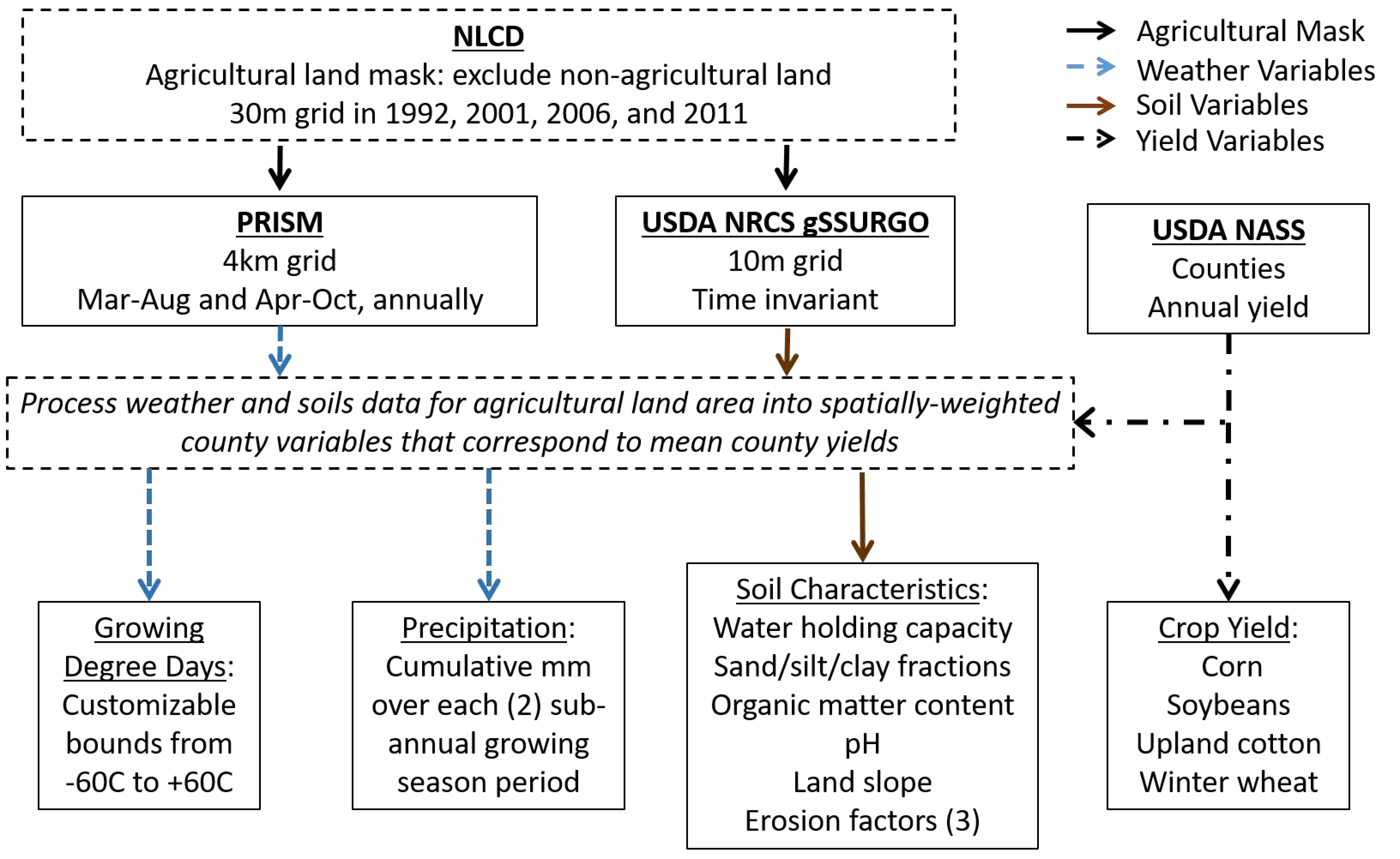
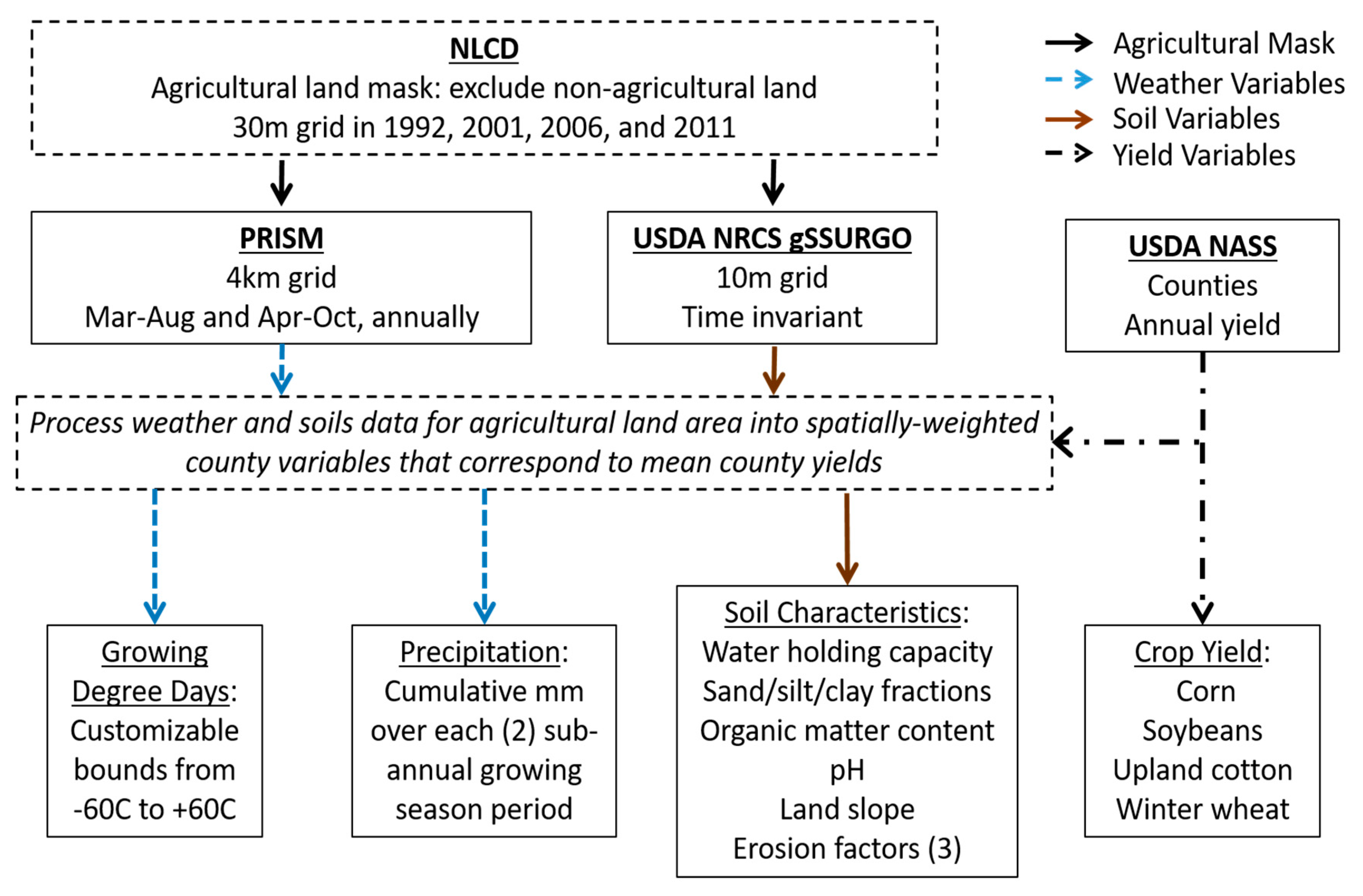
2.2. Data Inputs and Outputs

The ACDC data processing workflow from input data to output variables is summarized in the flow diagram in Figure 2 and filenames and variables linking data files are in

Table 1. ACDC data description (data file names are in italics).

Data Source/Filter	Crop Yields (bu/ac)	Weather		Soil
		GDD	Precipitation
USDA-NASS a	Corn, Soybean, Cotton, Wheat	-	-	-
NLCD ag land mask	-	1992, 2001, 2006, and 2011
PRISM	-	Daily min/max + sine method = 1 °C interval	Daily total precipitation (mm)	-
gSSURGO	-	-	-	Soil composition (sand, clay, silt in %); Slope (m); Soil pH; Organic matter (%); K-factor; T-factor (tons/acre/yr); available water capacity (cm/100 m2)
Area weighted	-	NLCD-PRISM bridge file b	NLCD-PRISM bridge file b	-
Dataset file name	yielddata.csv	gddMarAug.csv gddAprOct.csv	pptMarAug.csv pptAprOct.csv	soil1992.csv; soil2001.csv; soil2006.csv; soil2011.csv;
Bridge variable(s) c	stco, year	stco, year	stco, year	stco

^a Geographical boundary is based on 2012 Agricultural Census; ^b NLCD-PRISM bridge file gridInfo.csv provided; ^c All provided data sets can be merged as desired using the bridge variables.

.

Among the many agricultural outputs available from the USDA-NASS, ACDC provides county-level crop yields (bu/ac) for four major field crops. Crop yield data are contained in <yielddata.csv> in the ACDC pack in Table 1 (see Appendix A for the output file names and the associated variable names and definitions). Following [9], two growing season periods from March to August and April to October of each year throughout 1981–2015 are included in the climate data sets. As shown in Table 1, weather variables calculated over these two growing periods are provided in the files titled <xxMarAug.csv> or <xxAprOct.csv>, where xx is “gdd” for growing degree days (GDD) or “ppt” for precipitation data.

The NLCD is a 30-meter resolution raster file including the land cover and land-use information available for 1992, 2001, 2006, and 2011. To construct ACDC these four NLCD data years were used as agricultural land use masks to exclude non-agricultural land areas when extracting weather (PRISM) and soil variables (gSSURGO box in Figure 2). To provide the most realistic agricultural mask over time, ACDC allocated the 35 years of PRISM data to the periods 1981–1995 (1992 NLCD), 1996–2003 (2001 NLCD), 2004–2008 (2006 NLCD), and 2009–2015 (2011 NLCD). Due to the difference in grid sizes between PRISM (4 km) and gSSURGO (10 m) data, ACDC uses different ways of raster calculation to mask out non-agricultural areas from weather and soil data as depicted in Figure 3.

In Figure 3, the left panel is Tunica County (solid line) in Mississippi from the 2012 Agricultural Census county map overlaid on the 2011 NLCD. The right two panels are the 709640-th 4 km × 4 km cell of the national PRISM grid. The center panel displays the 30 m × 30 m NLCD agricultural grid cells within that PRISM cell (brown cells for agriculture, blue cells for non-agriculture). Because the NLCD resolution (30 m) is finer than PRISM (4 km), the weighted averages of the agricultural areas are necessary to calculate county-level weather variables that only account for the agricultural area in a county. For this purpose, ACDC provides the number of 30 m × 30 m NLCD agricultural grid cells within each 4 km × 4 km PRISM grid cell. Note that all cells in the NLCD grid have the same area (900 m²), and therefore it is possible to use the number of agricultural NLCD cells to calculate the area weights of PRISM weather variables within a county. In practice, only fractional amounts of some NLCD (PRISM) cells may fall inside a given PRISM cell (county boundary) and such cases require area weights attributed to agricultural land areas to take these partial cell areas into account. The total agricultural land area in each NLCD cell within a PRISM cell is aggregated and divided by the total agricultural land area within each PRISM cell to calculate the agricultural land area weight (land share) that is then multiplied by each weather variable for all PRISM cells located inside a county and summed to get an area-weighted county-level value for each weather variable in each time period. The NLCD-PRISM bridge file in Table 1 is provided as <gridInfo.csv> (details in Appendix A

Table A2. <gridInfo.csv> variables.

Variable Name	Description
gridNum	PRISM grid cell index under NLCD projection
stco	State FIPS + county FIPS (detailed codes in 2012 Agricultural Census)
numAg1992	number of agricultural cells based on 1992 NLCD
numAg2001	number of agricultural cells based on 2001 NLCD
numAg2006	number of agricultural cells based on 2006 NLCD
numAg2011	number of agricultural cells based on 2011 NLCD

) in the ACDC file package, which includes gridNum for the unique PRISM grid number, stco for the State and County FIPS codes, and numAg1999, numAg2001, numAg2006 and numAg2011 for the numbers of agricultural NLCD grids for each NLCD year.

Unlike the PRISM grids, the resolution of the gSSURGO data are finer than the NLCD. To calculate soil characteristics only for the agricultural area, ACDC first overlays6 gSSURGO (10m resolution) on the NLCD (30m resolution) using the nearest neighbor method (see Appendix B: ESRI, 2016), and then the average values of different soil characteristics are calculated for the projected map unit (MAU) in gSSURGO. In Figure 3, the average of the gSSURGO colored areas (green and light-pink) are only taken to calculate the soil variable values in Tunica County. Using four NLCD years, the major soil variables relevant for agro-climatic relations are provided in the file <soilYEAR.csv> in ACDC (

Table A5. <soil1992.csv>, <soil2001.csv>, <soil2006.csv>, and <soil2001.csv> variables.

Variable Name	Description
stco	State FIPS + county FIPS (detailed codes in 2012 Agricultural Census)
whc	available water capacity (cm/100 m2) (awc in gSSURGO)
sand	sand proportion (%) (sandtotal in gSSURGO)
silt	silt proportion (%) (silttotal in gSSURGO)
clay	clay proportion (%) (claytotal in gSSURGO)
om	organic matter in 2 mm top soil (%) (om in gSSURGO)
kwfactor	soil erodibility factor by water adjusted for rock fragments (kwfact in gSSURGO)
kffactor	soil erodibility factor by water (kffact in gSSURGO)
spH	soil pH (ph1to1h2o_r in gSSURGO)
slope	slope (m) (slopelenusle in gSSURGO)
tfactor	soil loss tolerance factor (tons/acre/yr) (tfact in gSSURGO)

in Appendix A), where YEAR is 1992, 2001, 2006 or 2011. The calculation details for each variable follow in the next section.

3. Material and Methods

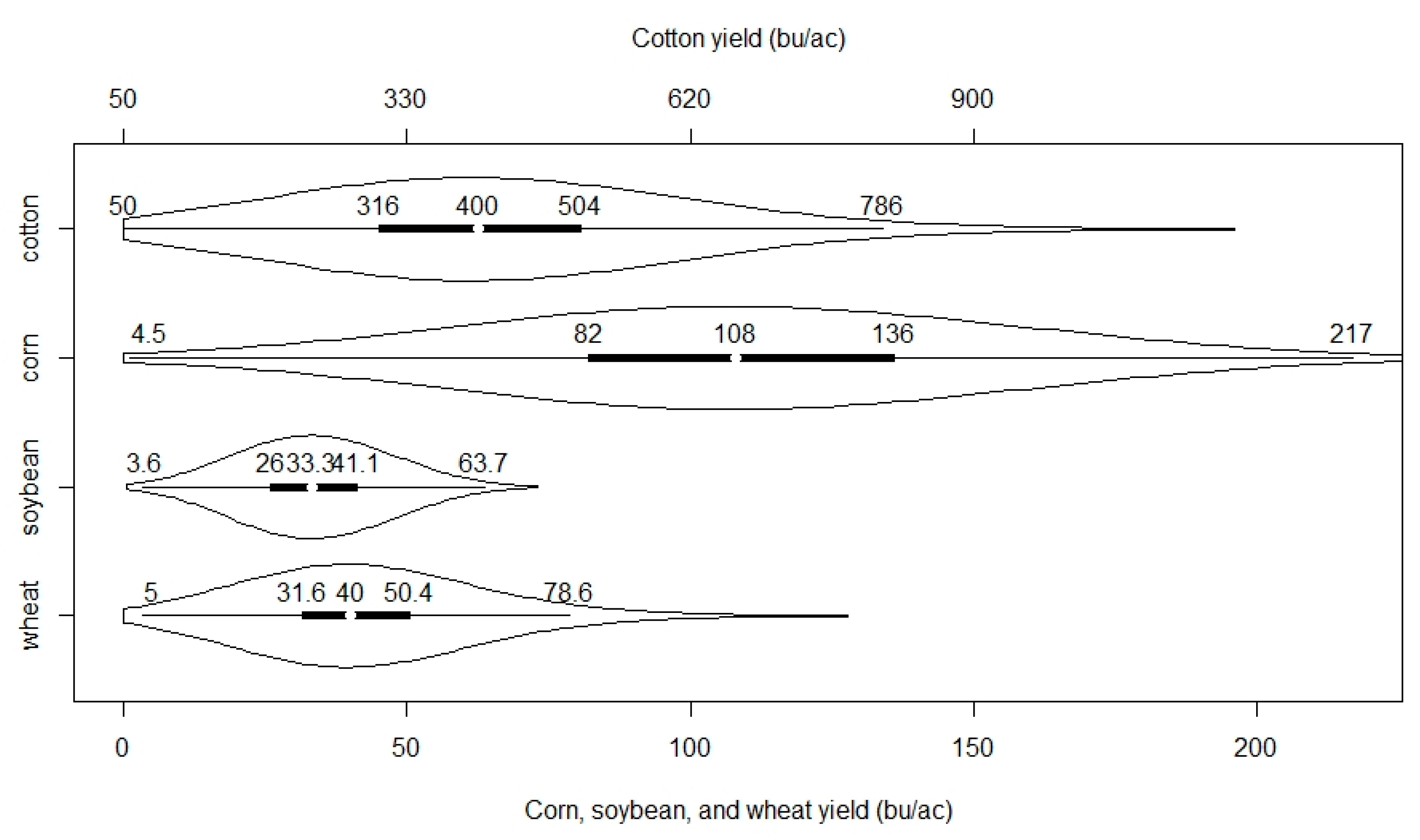
3.1. Crop Yields

The USDA-NASS yield data for 1981–2015 are included in ACDC (v.1.0.0) to match PRISM data availability and be consistent with the climate “normal” in a location based on ~30 years of weather data. Descriptive statistics are described in Figure 4.

Each violin plot in Figure 4 consists of the Gaussian kernel densities and boxplots for each crop. Due to yield value size differences, cotton is presented on a different scale from the other crops on the secondary horizontal axis. All four crops are measured in bushels per acre (bu/ac) provided in the USDA-NASS yield data. Excluding cases with no records (counties or crops without NASS data in a given year have NA values in the data), ACDC includes 35 years of yield data in 107,450 observations drawn from 3070 counties. Figure 4 summary statistics reflect 70,721 observations for corn, 56,960 observations for soybean, 15,668 observations for cotton, and 55,848 wheat observations. Appendix A

Table A1. <yielddata.csv> variables.

Variable Name	Description
stco	State FIPS + county FIPS (detailed codes in 2012 Agricultural Census)
year	Year: 1981–2015
corn	corn yields (bu/ac): 1981–2015
soybean	soybean yields (bu/ac): 1981–2015
cotton	upland cotton yields (bu/ac): 1981–2015
wheat	wheat yields (bu/ac): 1981–2007

provides variable names for each crop included in the ACDC data package.

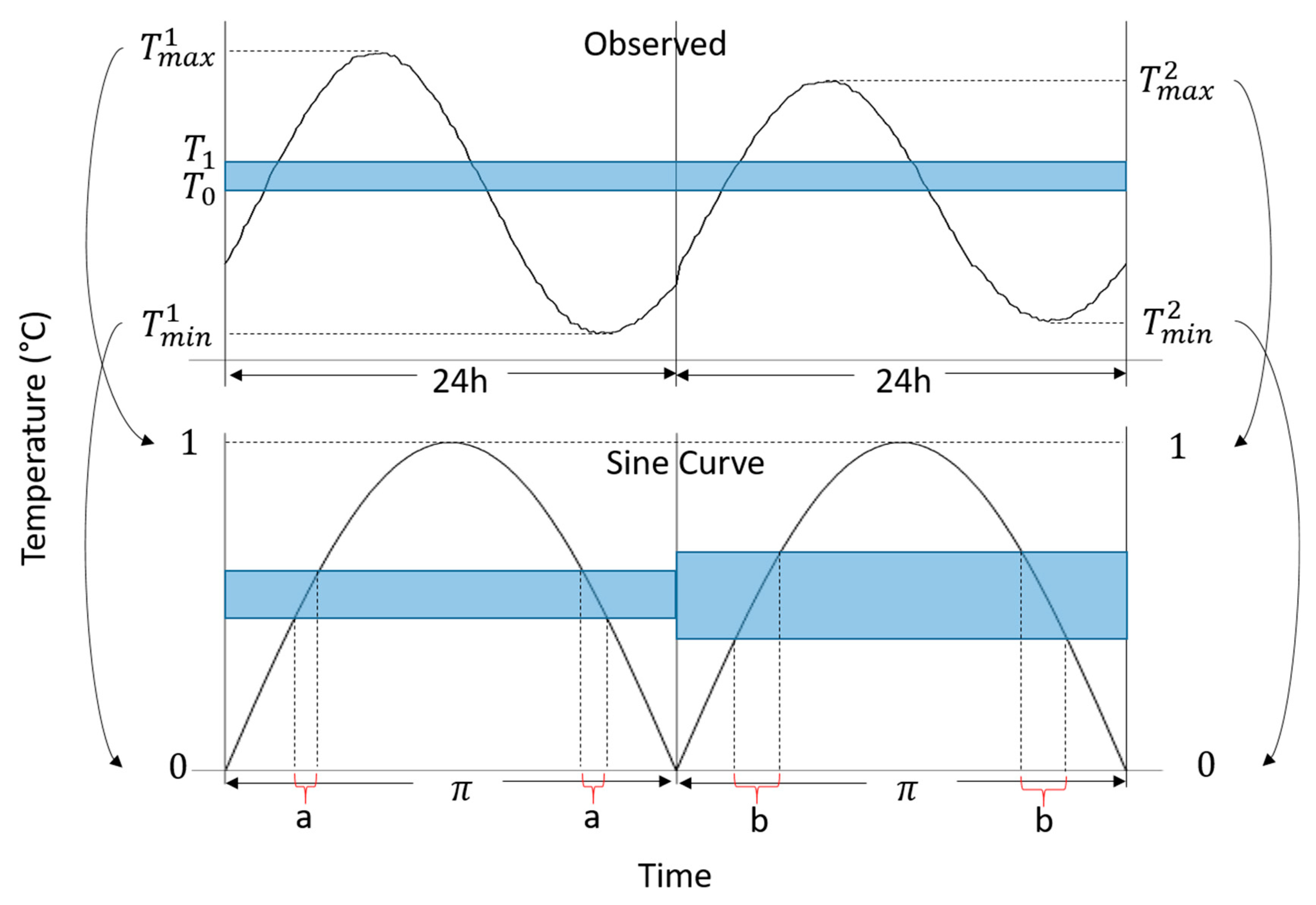
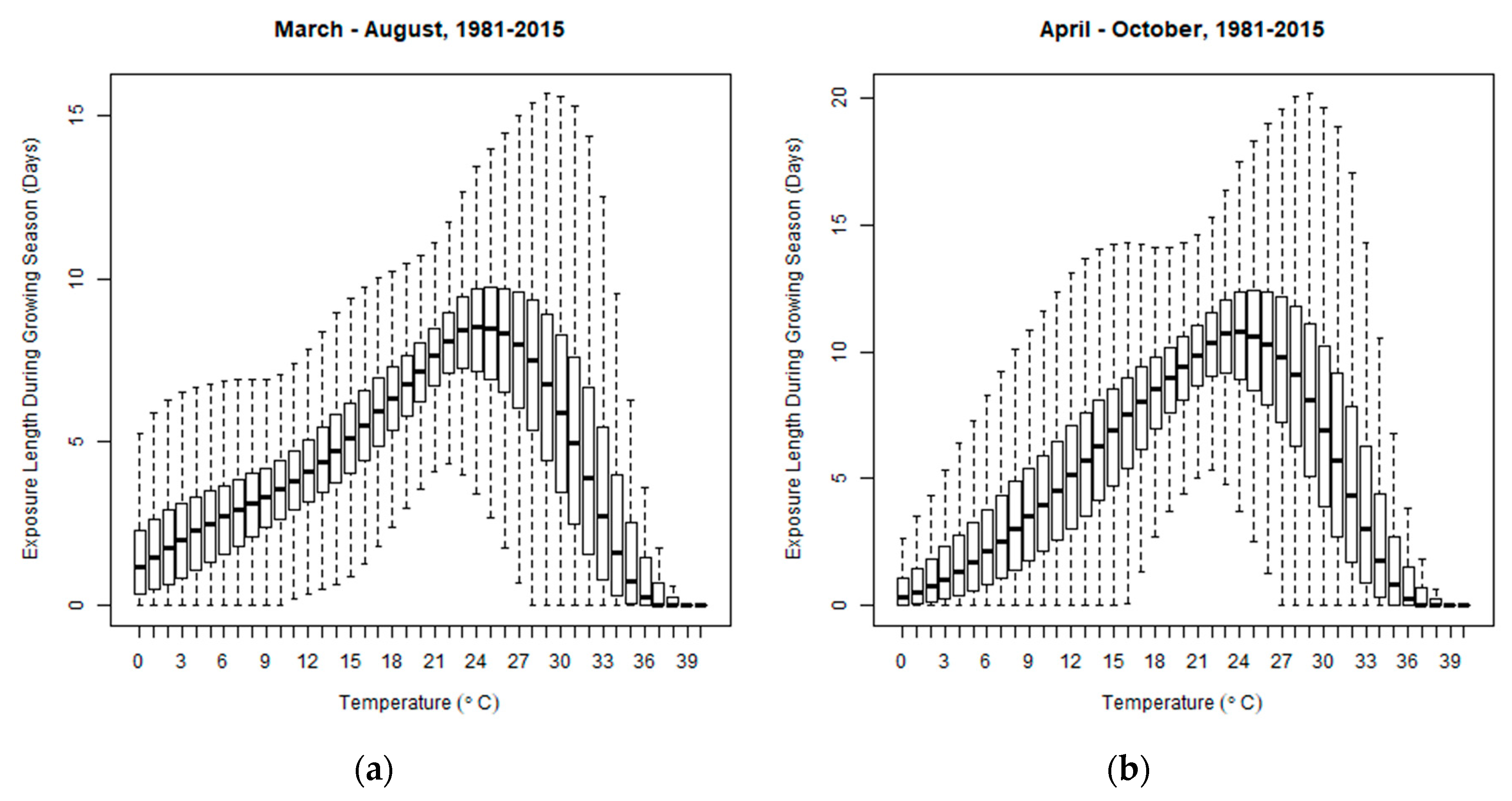
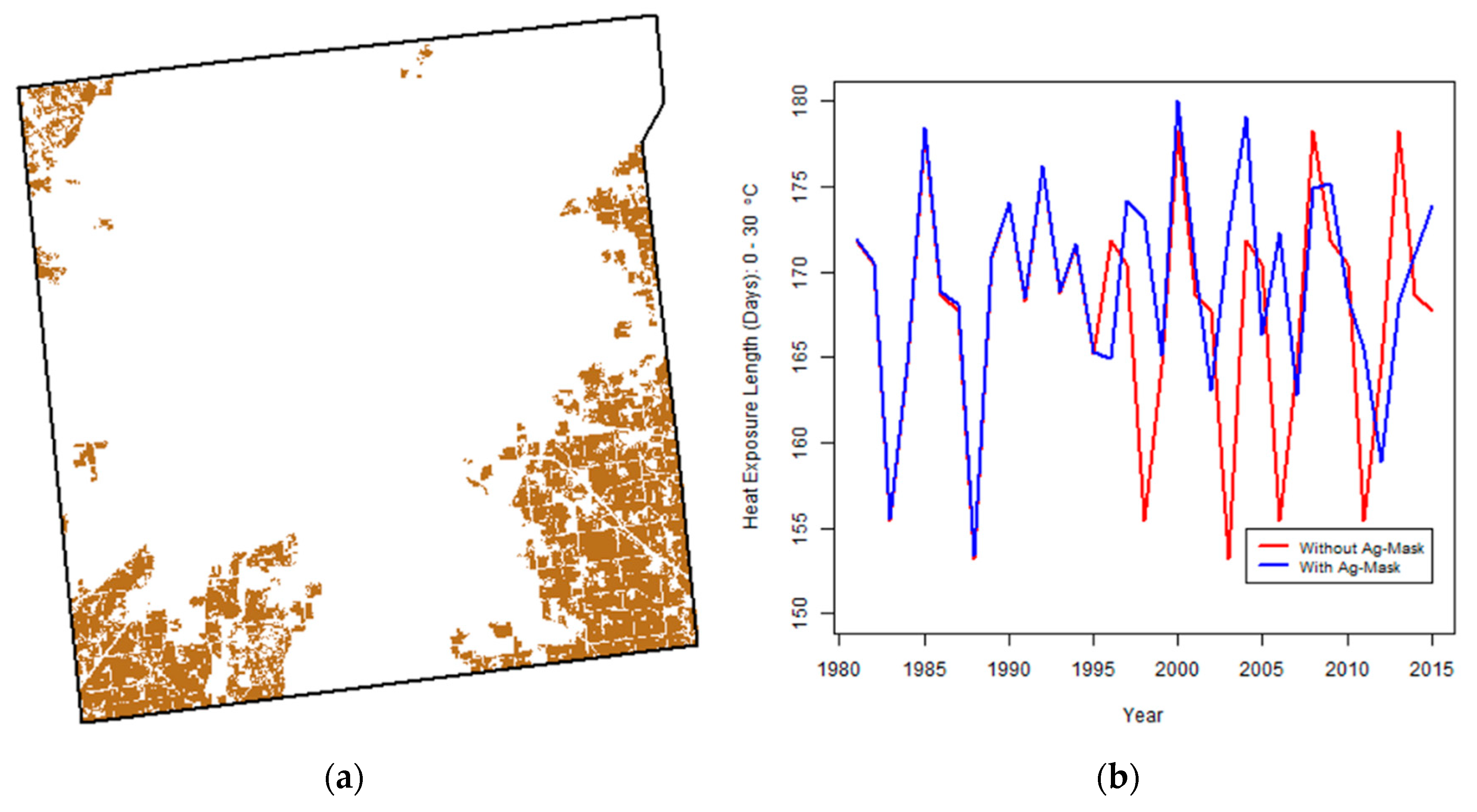
3.2. Heat Exposure Length

Temperature (or heat exposure) is an essential component controlling the developmental rate of crop organisms [13,14]. The total amount of heat required, between a lower and upper threshold, for crops to develop from one point to another in their life cycle is calculated in units called degree-days (°D) [14,15]. For example, 18 °C to 25 °C is the optimal heat exposure for annual crops [16]. A day of 19 °C, therefore, contributes 1°D. Each growth stage of a crop has its own total heat requirement and development can be estimated well for some crops by accumulating degree-days between the temperature thresholds throughout the growing season [15]. The total heat exposure measured in degree-days during the growing season (GDD: growing degree-days) is a popular measure of heat contribution to crop development [13,17]. It has been demonstrated that heat has a nonlinear impact on field crop yields and yield deviation [9,18]. Even though the average temperature and its squares are still pervasively used in the literature, the calculated GDD in detailed temperature intervals are an agronomically and biophysically better measure of heat units required for crop development.

Data on daily minimum and maximum temperatures measured during the growing season are essential to calculate GDD. PRISM provides both daily variables in each year since 1981. Using the daily maximum and minimum temperatures, various ways of estimating GDD have been suggested including the triangle method, sine method, Huber’s method, or cutoff method [15,17,19]. Considering its popularity and better estimation performances [17,19], ACDC used the sine method to calculate heat exposure time length for temperature intervals described in Figure 5.

In Figure 5, we assume two days PRISM maximum and minimum temperatures are given as $T_{max}^1$ and $T_{max}^2$ for the first and second day temperature maximum, and $T_{min}^1$ and $T_{min}^2$ for the first and second day temperature minimum. On the upper panel of Figure 5, we estimate the heat exposure time length of $T_1-T_0$ (blue-highlighted temperature interval) for both days. On the lower panel of Figure 5, two identical sine curves are assigned for both days. Note that the maximum and minimum temperatures are assigned to the maximum (1) and minimum (0) of the sine curves for both days. Because the second day has the smaller temperature difference between the maximum and the minimum than the first day does, the blue-highlighted area of the second day is larger than that of the first day in the lower panel of Figure 5. The time length (in $\mathsf{\pi }$-time units) exposed to a certain temperature range, therefore, is 2a on the first day and 2b on the second day. In equation form, the exposure time length (in days) can be calculated by Equation (2).

$$\mathrm{days}=\frac{2}{\mathsf{\pi }}\left(arcsin\left(\frac{T_1-T_{min}}{T_{max}-T_{min}}\right)-arcsin\left(\frac{T_0-T_{min}}{T_{max}-T_{min}}\right)\right),$$

(2)

where arcsin is the inverse of the sine function, i.e., the arc-sine function.

The total heat exposure length (in days) during the growing season provided in ACDC includes calculations for two different growing seasons: March to August and April to October. Using Equation (2), ACDC provides 1 °C interval total heat exposure length from −60 °C to +60 °C. As discussed around Figure 3, county level values are calculated by the agricultural area weighted average with <gridInfo.csv>. Boxplots for each set of growing season months are shown in Figure 6.

Close inspection of Figure 6 shows that April to October heat exposure length (b) has a thinner left-tail distribution than the March to August graph (a). In addition, Figure 6b (1981−2015) has a thicker temperature distribution above 21 °C than those of [9],7 which is based on the station data for 1950–2005. This reflects, consistent with climate change, how we have experienced higher temperatures in the most recent years compared to past years.

In ACDC (Appendix A

Table A3. <gddMarAug.csv> and <gddAprOct.csv> variables.

Variable Name	Description
stco	State FIPS + county FIPS (detailed codes in 2012 Agricultural Census)
year	Year: 1981-2015
gddm#	(m = negative, (−))−# Celsius degree days between −# ±0.5 °C
gdd0	0 Celsius degree days between −0.5 °C and +0.5 °C
gddp#	(p = positive, (+)) +# Celsius degree days between +# ±0.5 °C

), the variable names for these 1 °C heat exposures with ±0.5 °C are gddm#, gdd0, and gddp#, where m# denotes negative numbers, 0 is for zero and p# for positive numbers. For example, gddm10 presents the total days exposed to −10.5 °C ~ −9.5 °C, while gddp20 contains the total days exposed to 19.5 °C ~ 20.5 °C during the growing season. Because heat exposure days are additive, a user can simply make a summation of them for the desired interval that corresponds to the temperature range relevant to the crop or other plants of interest (not just those with yields in ACDC). For example, the summation of all degree days from gddp5 to gddp20 is for the heat exposure days between +5 °C and +20 °C. Using these heat exposure days, a user also can simply calculate GDDs by calculating the expected value of heat exposure days with Equation (3).

$$GD{D}_a^b={{\displaystyle \sum }}_{k=a}^b{h}_k\left(\frac{h_k}{{{\displaystyle \sum }}_{i=-60}^{60}{h}_i}\right),$$

(3)

where $GD{D}_a^b$ is the GDD between a °C and b °C, $h_k$ is the heat exposure days for the gddk variable in ACDC, and the last term in parenthesis is the relative frequency of $h_k$ over the whole growing season. Equation (3), therefore, provides the Riemann sum of heat exposure length curve over the entire duration of the growing season [15,17,19].

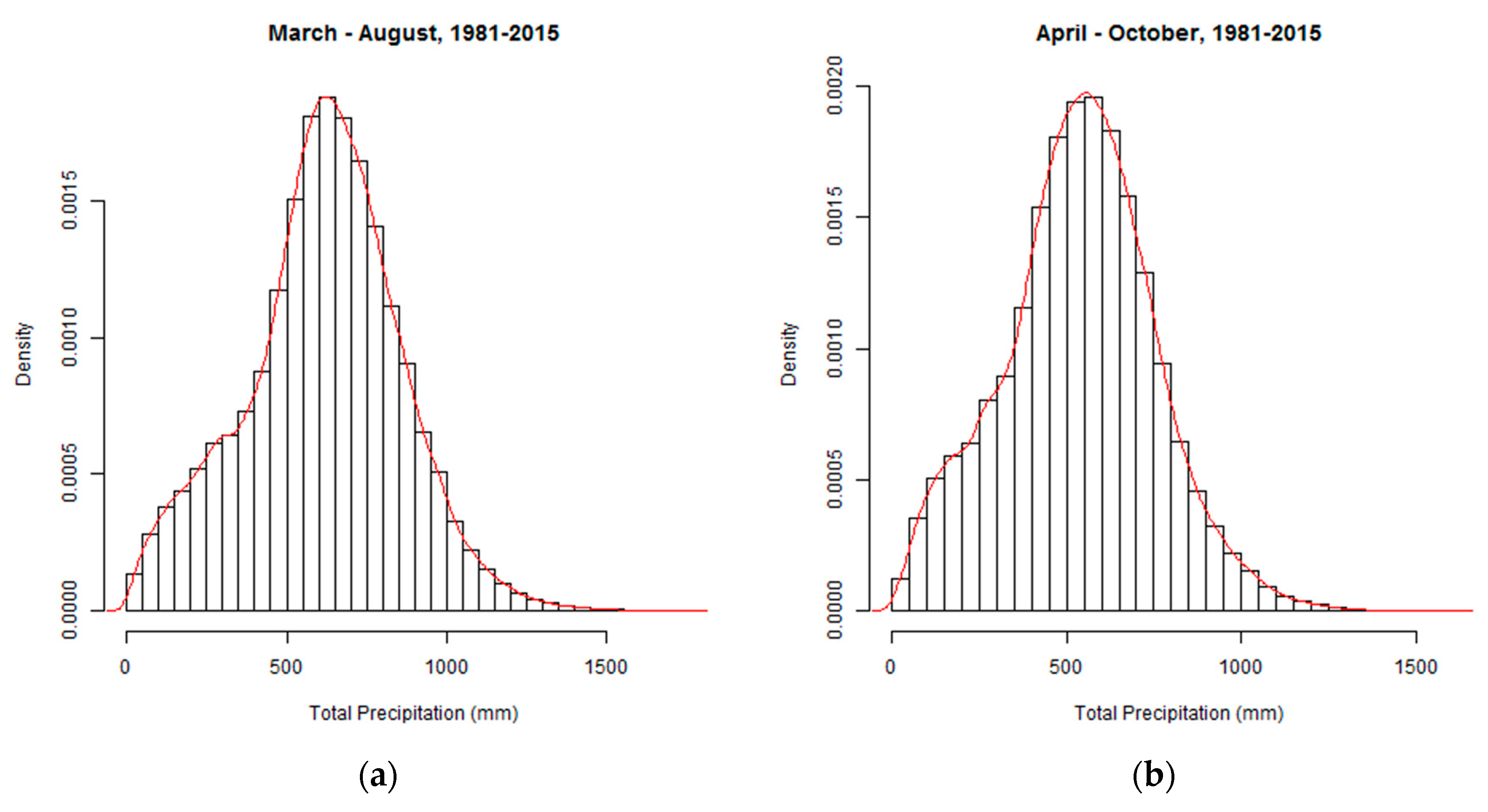
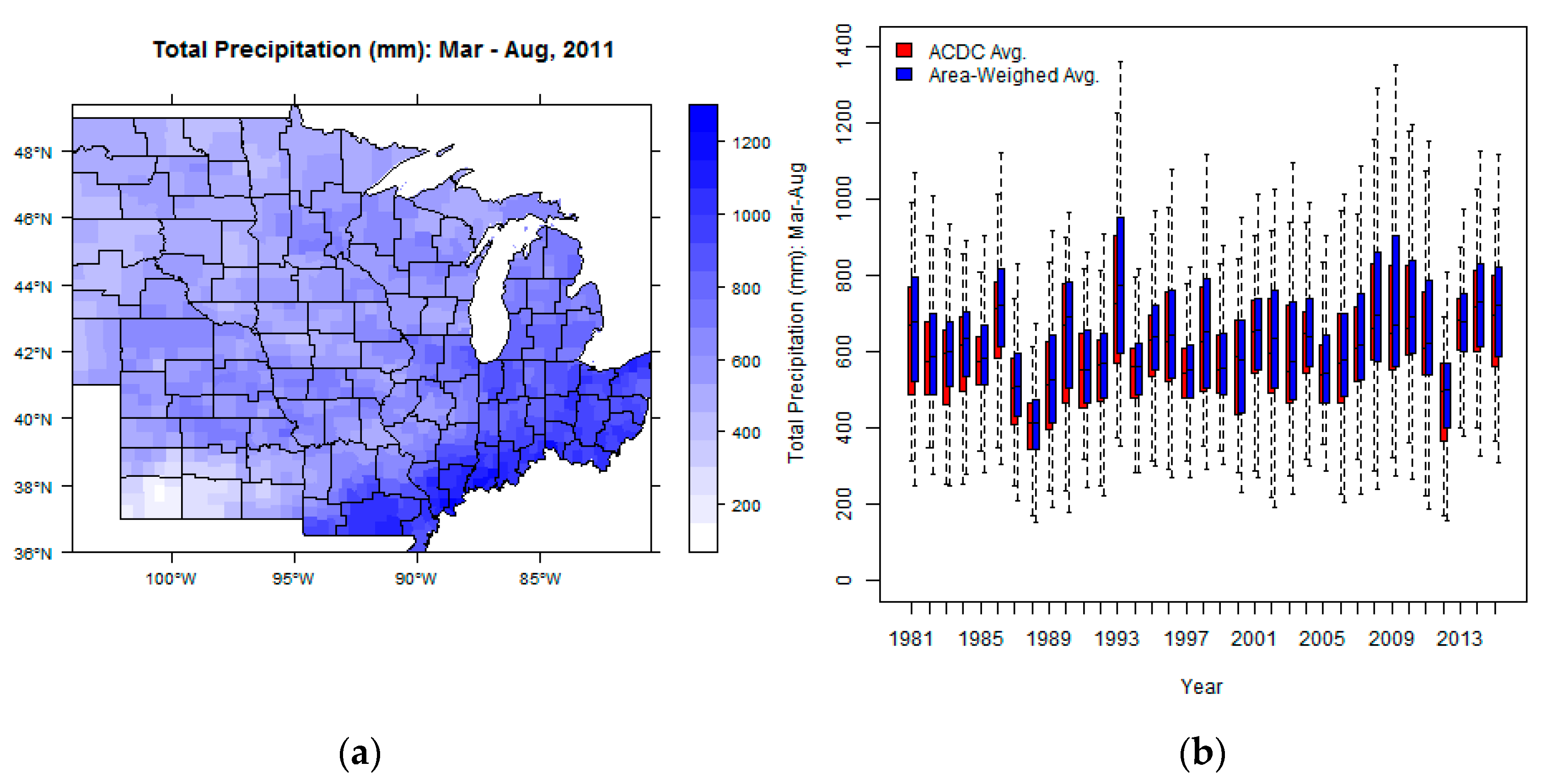
3.3. Total Precipitation

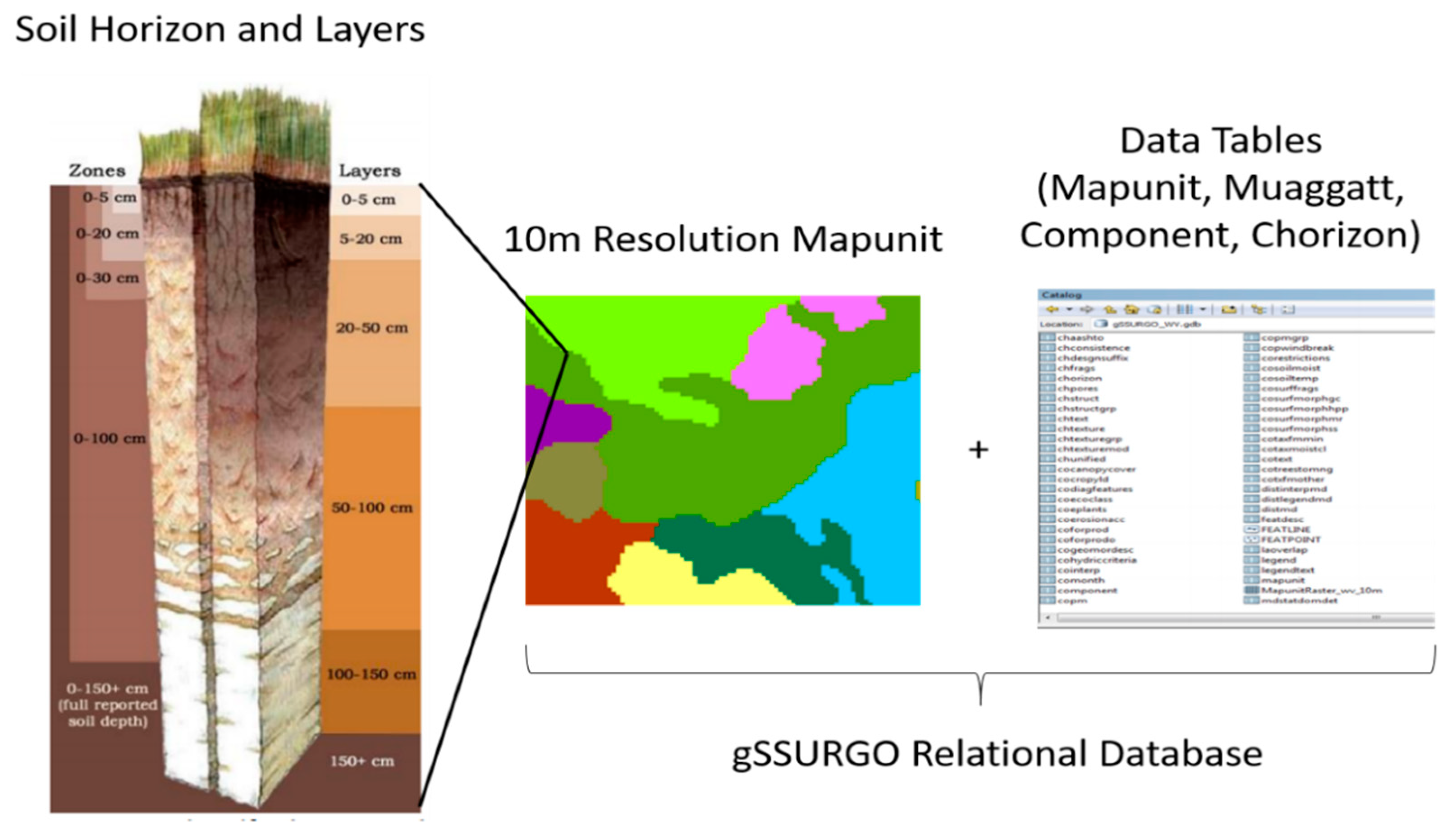
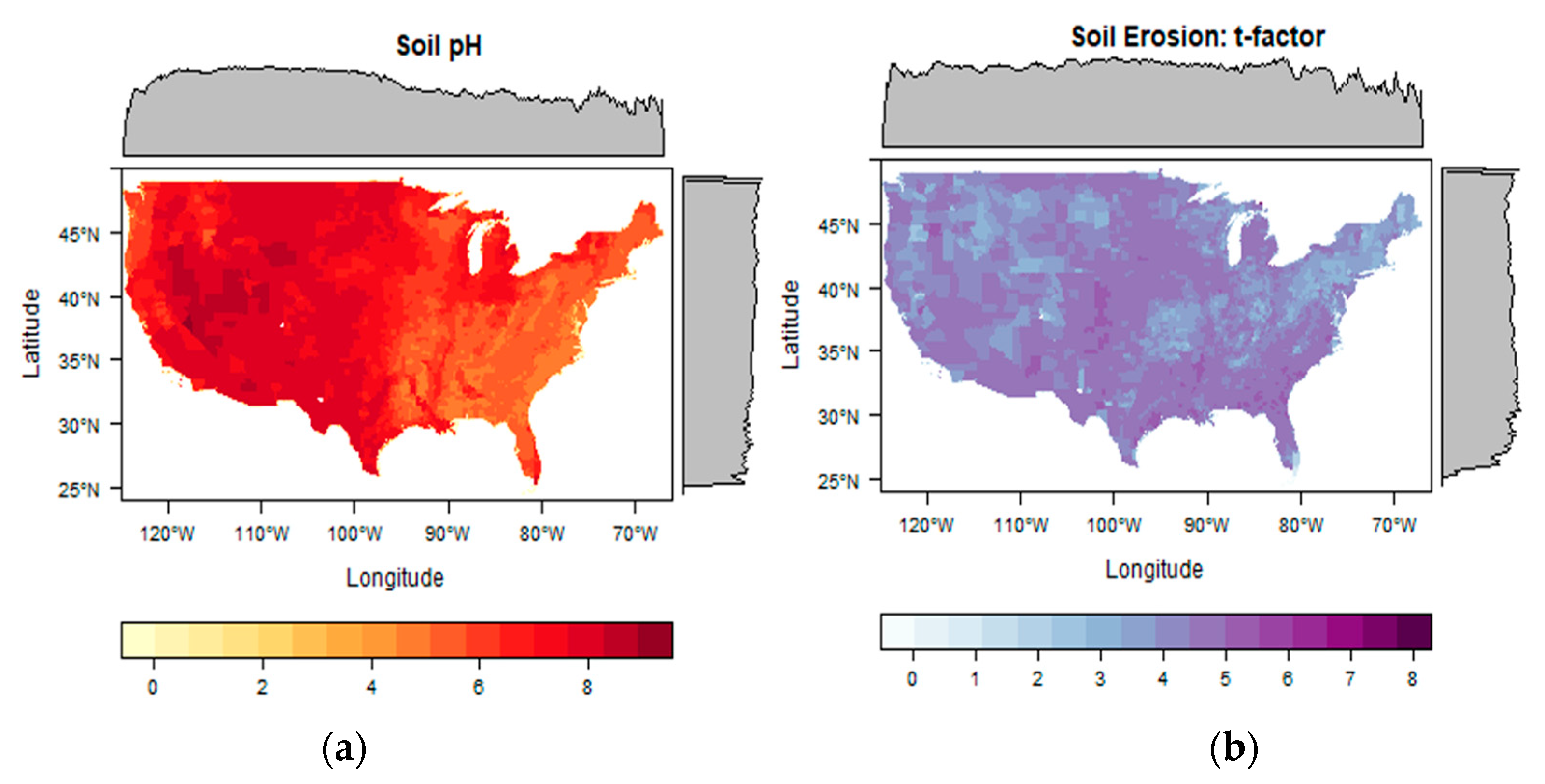
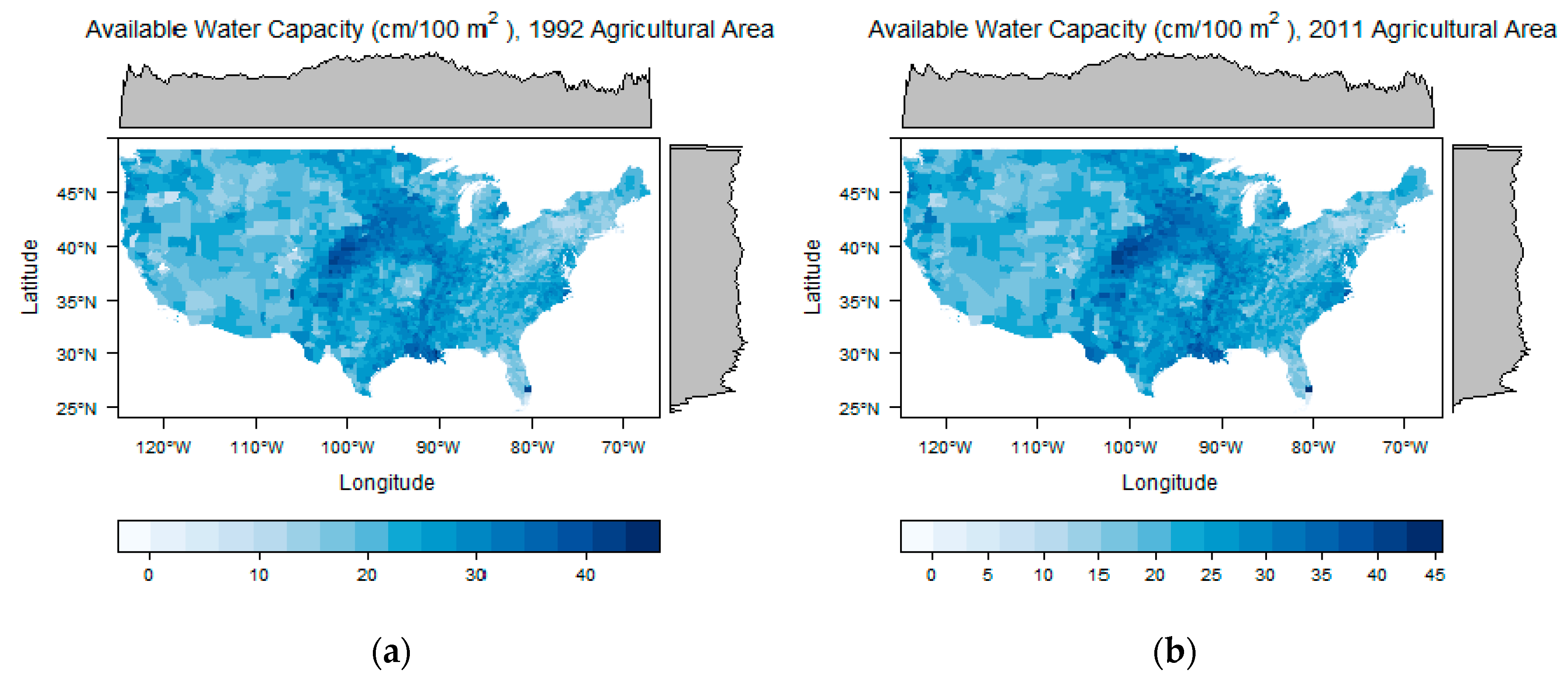
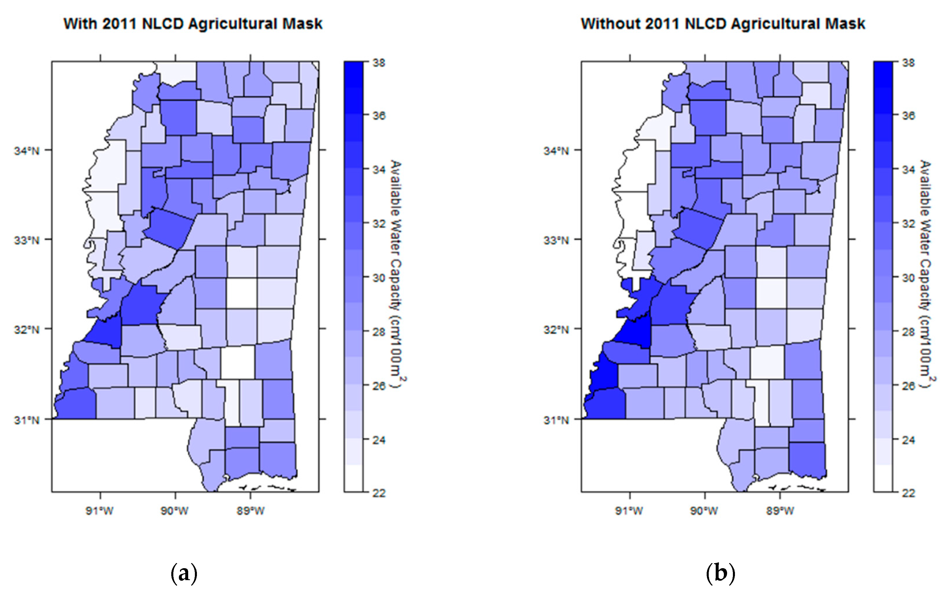
Total precipitation during the growing season is another important variable to describe agro-climatic relations. Using PRISM daily precipitation data, ACDC provides the total precipitation values for both growing seasons. To calculate the county total precipitation, the agricultural area weights contained in <gridInfo.csv> are applied. The variable ppt in ACDC is summarized by the distribution in Figure 7. As discussed in [18], the effect of total growing season precipitation on yield (or yield deviation) is not sensitive to its specification.

3.4. Soil Variables

Soil quality contributes significantly to crop development and yields [20,21,22]. Soil quality, however, is a general term that describes the overall condition of the soil with respect to its intended use [23]. In the agro-climatic models, various soil characteristics and variable specifications have been employed. For example, soil erosion factor can be slope [5], K-factor [24], or T-factor [25]. As [24] pointed out, a soil characteristic is used for calculating other soil variables, i.e., a soil variable is a function of other soil characteristics. An example is K-factor as a function of slope and profile-permeability. In regression-based analysis, this could be an issue of double counting (a source of endogeneity) discussed in [8]. Following the importance of soil characteristics on crop productivity discussed in [23], ACDC includes the following ten individual soil characteristics: available water capacity, soil texture (proportion of sand, silt, and clay), organic matter content, soil pH, slope, and soil erosion factors (K-factor, water adjusted K-factor, and t-factor). See Appendix A Table A5 for the ACDC variable names and basic details.

Soil characteristics in ACDC are based on the NRCS gSSURGO database. Because of the complexity of soil structure, gSSURGO variables are defined in the relational database by including 10 m resolution map unit and data tables of soil characteristics.8 Figure 8 is provided to facilitate an explanation of how data were processed from this complicated relational database. Soil characteristics vary at different depths. The left panel of Figure 8 presents different soil layers and horizons by depth. The raster map of gSSURGO is based on these soil volumes as 10 m resolution grid cells. Each grid cell of the gSSURGO raster in the center panel of Figure 8 is a 10 m × 10 m “mapunit” cell representing the soil horizon, layer, and chemical components at different depths from the soil surface. Grid cells in the center panel of Figure 8 that are the same color, therefore, share common soil characteristics. Each mapunit of the gSSURGO raster has a MUKEY that is a bridge variable linked to the data tables listed in the right panel of Figure 8. If a user connects the MUKEY of the mapunit of a grid cell, then all soil components at different depths can be drawn from the gSSURGO data tables.

Using these data tables and mapunits, ACDC includes calculated values for the ten soil characteristics mentioned above for the agricultural (only) land use areas within each county based on the NLCD. Because the resolution of gSSURGO is finer than the resolution of NLCD, ACDC selected only the gSSURGO mapunits located in NLCD agricultural cells. It is important to note that the gSSURGO database is composed of soil measures per unit of volume at different depths. To derive the county-level soil characteristics for ACDC, the soil layer thickness weighted average of the soil variables is calculated first. Second, the arithmetic spatial average of the thickness-weighted values within a county (as discussed around Figure 3) is calculated. As an example of the soil characteristics contained in ACDC, Figure 9 shows soil pH (a) and t-factor (b) from the ACDC based on the 2011 NLCD agricultural mask.

In light of farm management and conservation, soil quality and other characteristics are generally dynamic, likely varying by location over time in managed agricultural production areas. Due to the implausibility of widespread dynamic data collection, soil variables contained in NRCS soil survey data are generally assumed to be constant over time. In county-level analysis, in particular, soil characteristics are treated as time-invariant county-specific values using fixed effects terms in regression-based agro-climatic analysis [9,26]. ACDC soil data based on gSSURGO contains time-invariant soil variables from gSSURGO, however, because ACDC takes into account agricultural land use changes based on the NLCD (in 1992, 2001, 2006 and 2011), soil properties in each county do change over time as the land areas employed in non-forestry agricultural uses change over time. ACDC includes four different county-level soil characteristics tables titled <soilYEAR.csv> where YEAR is 1992, 2001, 2006 and 2011, but the temporal differences do not appear to be drastic and are hard to discern from national maps. In Figure 10, the maps of available water capacity (the area weighted depth of water covering a 10 m × 10 m cell, i.e., cm/100 m²) based on 1992 (a) and 2011 (b) agricultural masks are plotted. The general distribution of available water capacity on both maps is the same. The slight differences between the two maps in Figure 10, however, are observable in parts of California and darker blue areas in the Midwest. From the average density plots on both panels, the changes in county-level available water capacities between two years can be observed as well.

End-users of the ACAC should be cautious when using the spatial aggregation (or average) of soil variables, as the resulting soil variables may not make sense for a particular application or end-use of the ACDC data. To use the best practices possible, the authors consulted with soil scientists at their institutions to ensure that the procedures used to calculate variables to present county-level soil variation were appropriate. In the field of soil science and related disciplines, a common and often preferred way to utilize soil data is to work the single dominant-soil or split an area into smaller, more homogeneous spatial units.10

4. Discussion

ACDC is constructed from multiple widely-used raster databases to provide county-level variables prevalent in many agro-climatic research studies. Due to the required calculation methods and structure of the data sources employed in ACDC, many prospective users of these public data encounter unexpected and largely unavoidable data issues when trying to use these data sources, whether primarily for the purpose of research or application. In this section, three general issues when using the dataset or adopting the method in ACDC are discussed: agricultural mask, spatial aggregation and disaggregation, and computational burden.

4.1. Agricultural Mask

Individual raster data sources are based on equally-sized grid cells. The PRISM and gSSURGO data sets individually contain geo-spatial gridded data for the entire US, but each grid cell has a different size and neither gridded data set contains land-use information because these data are not the domain of PRISM or gSSURGO. Because land-use itself has a great influence on the environment and soil and weather data vary tremendously over space, using these data to conduct agro-climatic research without applying an agricultural land mask necessarily results in potentially large errors. To discuss the importance of agricultural masks in ACDC, Figure 11 is an example drawn from Marion County, IN where Indianapolis is located.

Figure 11a shows the agricultural (brown) and non-agricultural land use (white) areas in Marion County, Indiana, excerpted from the 2011 NLCD map. Due to the largely urban land-use surrounding Indianapolis, only about 20% of land within the county was used for agriculture in 2011. Figure 11b presents the average length of heat exposure, in days, to temperatures between 0 °C and 30 °C from March to August in the years 1981–2015. The blue line is calculated for only the agricultural land use areas (with the agricultural mask applied) in Figure 11b, while the red line is the simple average of all cells, regardless of land use, within Marion County (without the agricultural mask applied). It is clear that large differences in the level of heat exposure exist, depending on whether county mean heat exposure is calculated with or without taking into account the non-agricultural land area after 1995. These patterns of differences when masking out non-agricultural land uses vary by region and year. Therefore, not applying the agricultural mask could exaggerate or underestimate the actual yield response or other agri-environmental sensitivity in agro-climatic relations. This problem is not present when working with data at a single location (i.e., a specific farm field). It should be noted that the spatial interpolation method used to create the underlying gridded weather data may influence the effect of masking out non-agricultural lands on resulting weather variables and calculation of heat exposure or other variables based on the underlying weather data.

In the case of soil characteristics, the agricultural mask has a more significant impact in agro-climatic models than other variables do. Because soils are assumed to be invariant over time, the average values of soil characteristics without applying the agricultural mask are more likely to be inappropriate for agricultural production analysis than the agriculture only area is for time-varying weather. Figure 12 shows an example of available water capacity in Mississippi with and without the agricultural land mask (2011 NLCD map). About 30% of land in Mississippi is used for agriculture, therefore, the county-level values calculated without an agricultural mask are largely distorted toward non-agricultural lands. Figure 12 shows these distortions could be serious in soil variables; particularly the Mississippi Delta region (the northwest of the map that is the largest agricultural area of the floodplain of the Mississippi River). If the available water capacity values without the agricultural mask are used in a regression model of crop yield, the parameters will be biased due to the dominant non-agricultural land-uses. Due to the time-invariance of soil variables, in general, this bias will become worse if time fixed-effects are employed in longer time series.

Though not exhaustive, it should be clear from these examples involving weather and soil variables at the county and state levels that agro-climatic variables should be processed using an agricultural land mask to avoid introducing error before conducting agro-climatic analysis.

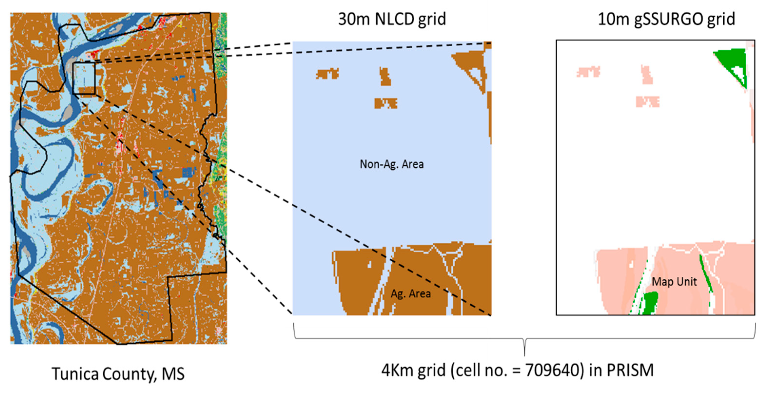
4.2. Aggregation and Disaggregation

ACDC provides the county level agro-climatic variables, but different agro-climatic data users will certainly want to work with other geographic boundaries, for example, USDA crop reporting districts (CRDs in [10]) or NOAA climate regions depending on the spatial resolution of the primary variable of interest. The aggregation or disaggregation of the county level data in ACDC is not recommended. Instead, the data should be reprocessed and aggregated following the same process used to construct ACDC for the needed geographical level to construct a spatially-consistent agricultural mask. This is necessary so that a spatially-consistent weighting scheme is used in matching gSSURGO, PRISM and NLCD grids to the desired aggregate spatial unit, whether smaller or larger than the county level.

In ACDC, the county-level weather data is built up as the area-weighted average. Aggregating up the counties to a CRD-level, for example, requires the average of the averaged values no matter what aggregation method is used. Because the average effectively smooths the data, masking underlying variability or extremes, the aggregation of ACDC will hide spatial variability compared to calculating values for higher levels of spatial aggregation (compared to counties) from the original data. This smoothing issue is shown in Figure 13. Figure 13a shows the total precipitation distribution (county-level data from ACDC) in twelve Corn Belt States during March to August 2011. The solid lines are the boundary of the USDA CRDs composed of groups of agriculturally similar counties in each state. If the CRD-level average (e.g., the area-weighted or arithmetic average) is directly calculated from the county-level values in ACDC, the county-level variations across counties in Figure 13a will be smoothed-out masking underlying variation over the entire CRD spatial unit. The average of the ACDC county values does not equal the agricultural area weighted average of a variable computed for the entire CRD. Close inspection of Figure 13b illustrates this by comparing the average of the averages (ACDC county data average in red) and the computed area-weighted average for each CRD (blue) across the Corn Belt States. Any simple aggregation of ACDC to larger spatial extents cannot be expected to give correct values, and is expected to result in a systematic reduction in overall variability.

Disaggregation of ACDC is also not recommended due to the lack of sub-county level information for value matching. For example, there is no information to properly match the ACDC county-level values to zip codes. Further, in going from higher to lower levels of spatial aggregation, there is the opportunity to reduce the aggregation bias that is necessarily introduced when building any spatially aggregated data set. Any downscaling assumption cannot possibly perform better than building a zip code level data set using zip code spatial boundaries from the original data sources. Therefore, in both aggregation and disaggregation of ACDC, this study recommends that users start from the original data sources.

4.3. Computational Burden and Required Resources

The geo-computations performed on the raw raster data sources to construct the ACDC data set require memory-intensive and time-consuming calculations. The motivation for creating ACDC is to allow prospective data users to avoid this computational burden, but the process of working directly from the raw raster data and performing the necessary geo-computational steps from scratch are described to document this process. For the interested reader who may seek to undertake their own customized data set creation or work with the raw data sources employed, we describe the calculation requirements to give an idea of the nature of the required computational burden involved.

All data generation for ACDC was implemented on R 3.3.2 and its compatible packages including rgdal, raster, rgeos, maptools, sp, and rasterVis. The 64-bit Windows 10 desktop machine used to create ACDC has a quad-core 2.80 GHz Intel CPU and 128 GB physical memory. Using all four cores, the parallelized R-code was run using the snowfall package for 27.32 min (for March–August, 1981–2015) and 29.11 min (for April–October, 1981–2015) to calculate the heat exposure length data. Because gSSURGO data are provided for each state individually, parallel computation of each state’s soil characteristics was performed using an individual core for each state. Therefore, the calculation time varied by the size of each state. The soil characteristics based on the 2011 NLCD for Texas, the largest state, took 39 h and 48.21 min compared to Rhode Island, the smallest state, which took 37.21 min to completely process. The total computation time required for 3070 counties covering 48 states and four NLCD years of soil characteristics was about three weeks. The rest of the variables were calculated using a single core and took several seconds each to complete. To manage the more time- and resource-intensive calculations above, the vectorization (using apply-family) of codes could perform faster in R. If high performance computing resources are available, users can reduce the total calculation time considerably.

During raster-computation over the conterminous United States, managing the RAM and temporary files properly becomes important. For example, the raster of 2011 NLCD is about 17 GB. Therefore, it is infeasible to work with a single 8 GB memory to import one NLCD map. Note that the total size of a daily PRISM variable for a growing season is approximately 44.6 GB or more even though the size of one raster of PRISM is about 3.5 MB. Therefore, an efficient programmer is not likely to write the code assigning unnecessary rasters to the memory during each step of geo-computation. Moreover, raster calculations like crop and mask generate several temporary files having .grd or .gri extensions that are generally bigger than the size of the original working raster file; if the programmer does not remove them properly, the hard disk storage will be filled up very quickly. For example, in the process of generating the ACDC data, calculating the first two-year county-level heat exposure length with PRISM data generates approximately 300 GB temporary files. It is impossible to finish this calculation for the whole 35 years (1981–2015) while keeping all these temporary files if there is not about 1.5 TB storage available. Prospective users of geo-computation should manage memory by setting the path of the temporary file at the beginning of the code and insert code to remove the temporary files after finishing intermediate calculations that require those files.

5. Conclusions

To improve researcher efficiency and accessibility on data preparation work, ACDC was designed to provide the most widely-used variables in the agro-climatic literature including crop yields, weather variables, and soil characteristics for the 3070 contiguous US counties (1981–2015). The variables in ACDC are constructed from the widely-used high resolution gridded data sources PRISM, gSSURGO, and NLCD. In this paper, data generating processes are discussed in detail along with the ACDC data structure, the role of agricultural land use mask, and potential data management issues. All ACDC variables are provided in comma-separated values (csv) format files and ACDC users are generally expected to combine these csv files using the bridge variables identified in this paper and the data documentation to meet their individual data needs. The ACDC data are intended to be particularly useful to prospective data users that would like to avoid the time burdens and computational resource requirements required to conduct geo-computation using the original data structures available from the original sources.

Though the current version of ACDC (v.1.0.0.) provides many of the major variables used in agro-climatic models and empirical research today, there is likely to be demand for additional variables and years in the future. The developers plan to update ACDC to meet future data needs as updated data become available. The most certain near-term update will be to add crop and weather data based on the soon to be released agricultural land use data after constructing an updated agricultural land mask based on the 2016 NLCD. The Multi-Resolution Land Characteristics Consortium (MRLC) has announced the new 2016 NLCD will become available soon. Depending upon their availability, weather and soil variables will also be updated (to v.2.0.0) based on the new agricultural land mask. This anticipated update will include additional years of crop yields and weather after 2015, and updated soil characteristics based on the 2016 NLCD agricultural land mask. As updates with additional years of PRISM weather raster data are made for heat exposure and precipitation, additional weather variables will be added to ACDC. Some planned additions include vapor pressure deficit (available in PRISM) and a drought index (computable from many sources). Additional agricultural crop yields accessible from USDA-NASS will also be added in future releases. ACDC will follow-up on data requests from end-users based on user demand. All future updates will be freely accessible from the ACDC repository.

References

1. IPCC (Intergovernmental Panel on Climate Change). Summary for Policymakers. In Climate Change 2014: Mitigation of Climate Change. Contribution of Working Group III to the Fifth Assessment Report of the intergovernmental Panel on Climate Change; Edenhofer, O., R. Pichs-Madruga, Y., Sokona, E., Farahani, S., Kadner, K., Seyboth, A., Adler, I., Baum, S., Brunner, P., Eds.; Cambridge University Press: Cambridge, UK, 2014. [Google Scholar]
2. McCarl, B.A.; Thayer, A.W.; Jones, J.P.H. The Challenge of Climate Change Adaptation for Agriculture: An Economically Oriented Review. Am. J. Agric. Econ. 2016, 48, 321–344. [Google Scholar] [CrossRef]
3. Deschênes, O.; Greenstone, M. The Economic Impacts of Climate Change: Evidence from Agricultural Output and Random Fuctuations in Weather. Am. Econ. Rev. 2007, 97, 354–385. [Google Scholar] [CrossRef]
4. Le, T.T.H. Effects of Climate Change on Rice Yield and Rice Market in Vietnam. Am. J. Agric. Econ. 2016, 48, 366–382. [Google Scholar] [CrossRef]
5. Hendricks, N.P.H.; Smith, A.; Sumner, D.A. Crop Supply Dynamics and the Illusion of Partial Adjustment. Am. J. Agric. Econ. 2014, 96, 1469–1491. [Google Scholar] [CrossRef] [Green Version]
6. Mendelsohn, R.; Nordhaus, W.D.; Shaw, D. The Impact of Global Warning on Agriculture: A Ricardian Analysis. Am. Econ. Rev. 1994, 84, 753–771. [Google Scholar]
7. Holzworth, D.P.; Snow, V.; Janssen, S.; Athanasiadis, I.N.; Donatelli, M.; Hoogenboom, G.; White, J.W.; Thorburn, P. Agricultural Production Systems Modelling and Software: Current Status and Future Prospects. Environ. Model. Softw. 2014, 72, 276–286. [Google Scholar] [CrossRef]
8. Dell, M.; Jones, B.; Olken, B. What Do We Learn from the Weather? The New Climate-Economy Literature. J. Econ. Lit. 2013, 52, 740–798. [Google Scholar] [CrossRef]
9. Schlenker, W.; Roberts, M.J. Nonlinear Temperature Effects Indicate Severe Damages to U.S. Crop Yields under Climate Change. Proc. Natl. Acad. Sci. USA 2009, 106, 15594–15598. [Google Scholar] [CrossRef]
10. Yun, S.D.; Gramig, B.M. Days Suitable for Field Work in the US Corn Belt: Climate, Soils and Spatial Heterogeneity. In Proceedings of the 2016 Annual Meetings of Agriculture & Applied Economics Association, Boston, MA, USA, 31 July–2 August 2016. [Google Scholar]
11. Rosenzweig, C.; Elliott, J.; Deryng, D.; Ruane, A.C.; Müller, C.; Arneth, A.; Boote, K.J.; Folberth, C.; Glotter, M.; Khabarov, N.; et al. Assessing Agricultural Risks of Climate Change in the 21st Century in a Global Gridded Crop Model Intercomparison. Proc. Natl. Acad. Sci. USA 2014, 111, 3268–3273. [Google Scholar] [CrossRef] [PubMed]
12. Villoria, N.B.; Elliott, J.; Müller, C.; Shin, J.; Zhao, L.; Song, C. Rapid Aggregation of Global Gridded Crop Model Outputs to Facilitate Cross-disciplinary Analysis of Climate Change Impacts in Agriculture. Environ. Model. Softw. 2016, 75, 193–201. [Google Scholar] [CrossRef]
13. Baskerville, A.G.L.; Emin, P. Rapid Estimation of Heat Accumulation from Maximum and Minimum Temperatures Published by: Ecological Society of America. Ecology 1969, 50, 514–517. [Google Scholar] [CrossRef]
14. Wilson, L.T.; Barnett, W.W. Degree-days: An Aid in Crop and Pest Management. Calif. Agric. 1983, 37, 4–7. [Google Scholar]
15. Zalom, F.; Goodell, P.; Wilson, L.T.T.; Barnett, W.; Bentley, W. Degree-days, the Calculation and Use of Heat Units in Pest Management. In University of California Division of Agriculture and Natural Resources Leaflet 21370; University of California: Berkeley, CA, USA, 1983. [Google Scholar]
16. Muchow, R.C.; Sinclair, T.R.; Bennett, J.M. Temperature and Solar-Radiation Effects on Potential Maize Yield across Locations. Agron. J. 1990, 82, 338–343. [Google Scholar] [CrossRef]
17. Thom, H.C.S. Normal Degree Days above any Base by the Universal Truncation Coefficient. Mon. Weather Rev. 1966, 94, 461–465. [Google Scholar] [CrossRef]
18. Roberts, M.J.; Schlenker, W.; Eyer, J. Agronomic Weather Measures in Econometric Models of Crop Yield with Implications for Climate Change. Am. J. Agric. Econ. 2013, 95, 236–243. [Google Scholar] [CrossRef]
19. Snyder, R.L. Hand Calculating Degree Days. Agric. For. Meteorol. 1985, 35, 353–358. [Google Scholar] [CrossRef]
20. Andrews, S.S.; Karlen, D.L.; Cambardella, C.A. The Soil Management Assessment Framework. Soil Sci. Soc. Am. J. 2004, 68, 1945–1962. [Google Scholar] [CrossRef]
21. Buman, R.A.; Alesii, B.A.; Hatfield, J.L.; Karlen, D.L. Profit, Yield, and Soil Quality Effects of Tillage Systems in Corn-Soybean Rotations. J. Soil Water Conserv. 2004, 59, 260–270. [Google Scholar]
22. Hess, G.R.; Campbell, C.L.; Fiscus, D.A.; Hellcamp, A.S.; McQuaid, B.F.; Munster, M.J.; Peck, S.L.; Shafer, S.R. A Conceptual Model and Indicators for Assessing the Ecological Condition of Agricultural Lands. J. Environ. Qual. 2000, 29, 728–737. [Google Scholar] [CrossRef]
23. Wolkowski, D. Soil Quality and Crop Production System. New Horiz. soil Sci. 2005. [Google Scholar]
24. Yun, S.D.; Gramig, B.M.; Delgado, M.S.; Florax, J.G.M.R. Does Spatial Correlation Matter in Econometric Models of Crop Yield Response and Weather? In Proceedings of the 2015 Annual Meetings of Agriculture & Applied Economics Association, San Francisco, CA, USA, 26–28 July 2015. [Google Scholar]
25. Montgomery, D.R. Soil Erosion and Agricultural Sustainability. Proc. Natl. Acad. Sci. USA 2007, 104, 13268–13272. [Google Scholar] [CrossRef]
26. Baylis, K.R.; Paulson, N.D.; Piras, G. Spatial Approaches to Panel Data in Agricultural Economics: A Climate Change Application. J. Agric. Appl. Econ. 2011, 43, 325–338. [Google Scholar] [CrossRef]
1
These high-resolution satellite imagery data often called raster data, grid-cell data, big data, or GIS data.
2
The full article is available from http://www.g-feed.com/2015/01/searching-for-critical-thresholds-in.html (retrieved 2/1/2018).
3
For the metadata description of these files, refer to: https://www.agcensus.usda.gov/Publications/2012/Online_Resources/Ag_Atlas_Maps/mapfiles/ag_co_metadata_faq_12.html (Accessed on 28 February 2017).
4
The NLCD projection is given by "+proj = aea + lat_1=29.5 +lat_2 = 45.5 + lat_0 = 23 + lon_0 = −96 +x_0 = 0 + y_0 = 0 + ellps = GRS80 + towgs84 = 0,0,0,0,0,0,0 + units = m + no_defs". The NLCD uses the Albers conical equal area, GRS 1980 Spheroid, NAD83 Datum. The detailed projection can be referred from https://www.mrlc.gov/faq_dau.php (retrieved 5 March 2018).
5
The PRISM releases daily data as an unstable form first, and then confirm them as stable form. Currently, a few years of the PRISM data after 2015 is available. These will be updated in ACDC for the next version.
6
The “overlay” is one of the raster calculation techniques to project one piece of raster data on a different resolution piece of raster data.
7
The first panel of Figure A1 in the appendix of [9] contains a figure comparable to the Figure 6a.
8
The USDA-Natural Resources Conservation Service provides the soils meta data information and documentation in detail: https://www.nrcs.usda.gov/wps/portal/nrcs/detail/soils/survey/geo/?cid= nrcs142p2_053631 (retrieved 28 February 2018).
9
The gSSURGO user guide can be accessed from the USDA-NRCS website: https://www.nrcs.usda.gov/wps/ PA_NRCSConsumption/download?cid=nrcseprd362255&ext=pdf, (retrieved 28 February 2018).
10
The authors thank an anonymous reviewer for pointing this out.
Figure 1. 2012 National Land Cover Database overlaid on 3070 contiguous Agricultural Census counties.
Data 04 00066 g001
Figure 2. Diagram of all output files with variables. The solid boxes are input/output data in ACDC. The dotted boxes are the processes including data management.
Data 04 00066 g002
Figure 3. Agricultural mask of NLCD (30 m resolution) on PRISM (4 km resolution) and gSSURGO (10 m resolution).
Data 04 00066 g003
Figure 4. Violin plots (Gaussian kernel density curves and boxplots) of crop yields: numbers are five boxplot values (minimum, first quartile, median, third quartile, and maximum from left to right) for each crop.
Data 04 00066 g004
Figure 5. Sine method of calculating temperature exposure length.
Data 04 00066 g005
Figure 6. Distributions of temperature exposure lengths (days), (a) March–August and (b) April–October, 1981−2015.
Data 04 00066 g006
Figure 7. Histograms of total precipitation (mm), (a) March–August and (b) April–October, 1981–2015.
Data 04 00066 g007
Figure 8. Diagram of gSSURGOsoil variable relationships (figures excerpted from the NRCS gSSURGO user guide9).
Data 04 00066 g008
Figure 9. (a) Soil pH and (b) t-factor data contained in <soil2011.csv>: the gray curves along each axis are the density plot of latitudinal and longitudinal averages.
Data 04 00066 g009
Figure 10. Available water capacity (cm/100 m2) in (a) 1992 and (b) 2011 with agricultural land mask.
Data 04 00066 g010
Figure 11. (a) Agricultural areas are brown and non-agricultural areas are whitel; (b) Heat exposure length (0–30 °C in days, March–August) with (blue line) and without (red line) agricultural land mask in Marion County, Indiana.
Data 04 00066 g011
Figure 12. Available water capacity (cm/100 m2) (a) with and (b) without agricultural mask in Mississippi State.
Data 04 00066 g012
Figure 13. (a) County-level total precipitation distribution (March to August, 2011) and (b) Average of county total precipitation (in red) and area-weighted average (in blue) for each CRD.
Data 04 00066 g013