Fast-Flux Dataset: Enhancing Cybersecurity Analysis and Defense

Abstract

A fast-flux network (FFN) keeps itself accessible by frequently altering its IP addresses, usually avoiding standard detection techniques. In April 2025, six countries released a joint advisory describing this method as a national security threat and calling on DNS providers to improve their detection analytics. Most existing datasets used for these analytics are outdated. This data descriptor presents a new fast-flux dataset compiled from confirmed fast-flux domains and two months of repeated DNS lookups. We used VirusTotal to find additional domains associated with each resolved address. The dataset contains 67,606 fast-flux domains and 23,924 legitimate domains taken from the top Alexa sites. For each domain and IP address, we record the geolocation, autonomous system number (ASN), and country. The dataset also includes a feature file consisting of 91,530 records and 20 features. It also includes the threat model, three analysis tasks, and evaluation results from various studies. A feature-definition forest trained with this protocol achieves 96.0% classification accuracy and serves as the reference baseline. We include the original JSON responses so users can examine or alter the feature definitions.

1. Introduction and Background

A fast-flux network ensures a domain name stays available even when the hosts behind it change, sometimes within a single TTL window. Although the domain remains accessible, the IP addresses do not, so a blocklist prepared based on yesterday’s resolutions becomes obsolete. In April 2025, six national cybersecurity agencies issued a joint advisory describing fast flux as a weakness in many networks and requesting that protective DNS providers develop accurate, timely fast-flux detection analytics. Reference [1]. MITRE ATT&CK lists the same behavior as a distinct one. The adversary technique [2] and the analytics used to detect it are trained and tested on data; most public datasets used for this were compiled ten years ago.

This data descriptor describes an open dataset created to fill this gap. The dataset started with 80 fast-flux domains previously confirmed in earlier work [3,4,5] and mentioned in tweets. Over a period of more than two months, we repeatedly resolved each domain and recorded the addresses in the DNS responses. We then used VirusTotal to check each address, identify other domains it hosted, and record the dates they were hosted. As a result, we obtained 67,606 fast-flux domains. We constructed the benign subset similarly by applying the same method to Alexa’s top-ranked list, which produced 23,924 domains. For each domain and address, we recorded the geolocation, ASN, and country to examine the distribution of FFN across networks and jurisdictions.

The archives, feature file, and collection code are provided under the CC BY 4.0 license; we include raw API responses alongside the derived features so users can recompute the features from the original records if needed. This paper serves as a data descriptor, as the dataset is the main artifact and the paper explains how it was constructed, what it contains, and its possible applications. Nothing new in the way of a detection method is presented; the random forest mentioned in Section 4.5 is included merely as a reference baseline.

We gathered the dataset to answer four questions that private collections in most published fast-flux studies cannot address.

(i)

Could a detector be trained and evaluated using a fixed and publicly available collection of fast-flux and harmless domains, in such a way that the two reported accuracies mean the same thing?

(ii)

What characteristics of a domain include the fast-flux signal when the spread, the registration history, the certificate history, and the file relationships are all available?

(iii)

To what extent can a detector be applied in difficult cases, that is, in legitimate domains which are also served from several addresses in several countries?

(iv)

What is the state of the supporting infrastructure for the reuse of addresses across campaigns, the concentration of registrars, and the lengths of time for which certificates are valid?

The feature file enables supervised learning to be carried out with respect to questions (i) to (iii), whereas for question (iv) access is needed to the raw records rather than to the labels. For this reason, we include the JSON archives together with the feature set. Section 4 converts the four questions into three defined tasks using a fixed evaluation protocol.

1.1. Threat Model

The adversary operates an online service that is subject to takedown efforts, which may include a phishing page, a malware distribution site, a command and control server, or an endpoint for data exfiltration [1]. The primary objective is to maintain service availability under adverse conditions, ensuring continued accessibility even if specific hosts are cleaned, blocklisted, or seized.

The adversary employs compromised hosts or rented proxies and maintains control over the DNS zone for at least one registered domain. The adversary can configure short time-to-live (TTL) values, provide different addresses in successive DNS responses, and continuously rotate the address pool. In single-flux operations, only A records rotate, whereas in double-flux operations, NS records also rotate. Additional tactics include registering multiple domains simultaneously, utilizing WHOIS privacy protection, selecting registrars with inadequate abuse management, and distributing the address pool across numerous autonomous systems and countries. The adversary may also imitate content delivery network behavior, as such activity is frequently perceived as benign.

The defender depends on the requirement for domain name resolution, as address rotation would otherwise remain undetected in DNS records. The adversary opportunistically assembles its address pool from compromised consumer hosts, including autonomous systems without commercial relationships. In contrast, content delivery networks may possess large address pools but are administratively unified. The dataset incorporates both adversarial and CDN patterns, enabling the model to learn to differentiate between them.

The defender may function as a recursive resolver, a protective DNS service, or a security operations center. This entity monitors DNS responses for queried domains and can enhance its analysis using passive DNS data and IP metadata. The defender lacks access to host telemetry or payload information and does not receive cooperation from the networks hosting the services. For each domain, the system must make a binary decision at or near the time of the query.

1.2. Background and Related Work

For almost 20 years, researchers have studied how to detect botnets, and the published methods fall into several categories depending on where they look for evidence, which is why they generally require different types of data [6,7]. Honeynets use decoy servers to attract attackers and reveal botnet structure [8]. Low-interaction honeypots simulate part of a system and limit the information the defender can obtain; Honeyd is a typical example [9]. High-interaction honeypots run a full system and show what the attacker does after the initial connection, and both scalable designs [10] and correlation analysis over honeypot networks [11] are based on this approach. Rather than depending on intrusion detection, this technique concentrates on spotting unusual network activity. Signature matching is precise but only catches things that have already been recorded [12], so anomaly detection methods keep an eye on behavior that does not conform to a host’s usual pattern; ensembles are used to improve accuracy [13] and applying a linear SVM in a hybrid fast-flux model helps to lower the false positive rate [14]. DNS-based detection monitors traffic anomalies caused by a botmaster when redirecting victims by applying rules to both the query and the response [15]. Mining-based detection uses machine learning on network traffic, usually after filtering and feature reduction [16]. Heuristic detection adjusts thresholds based on the traffic itself, for example, by identifying DNSBL reconnaissance queries while the campaign is still being set up [17].

Most research on fast flux has focused on passive DNS. Lombardo and others [4] combined several flux metrics derived from DNS traffic within a corporate network and identified addresses that were part of the Dark Cloud and SandiFlux networks. Zang and colleagues [3] worked higher in the DNS hierarchy using algorithmically generated names. Al-Duwairi and his team [5] developed PASSVM using features from a single DNS response message along with locally cached data, enabling the system to run fast enough for query time; an SVM with an RBF kernel reached 99.557% accuracy. Nagunwa and co-authors [18] proposed 56 features covering DNS, host, and network properties and attained 98.42% accuracy in the binary classification of fast-flux phishing hostnames. Ayo and his team [7] combined a rule-based genetic algorithm [19] with a k-nearest-neighbor classifier and achieved an accuracy in excess of 99%. Researchers have applied this approach to genetic search over the feature and parameter space [20] and have also applied deep hybrids such as CNN-LSTM to the more general botnet problem [21].

Recent studies have moved beyond fast flux to examine malicious domains more broadly. Silveira et al. [22] analyze domains that have just been registered in a TLD by means of the first DNS query, using a combination of supervised models and clustering, and obtain an AUC of 0.962. Shafi et al. [23] introduce a DNS-flow abstraction incorporating more than 120 application-layer features and make the BCCC-CIC-Bell-DNS-2024 dataset available. Chandra et al. [24] build a graph showing the relationships between domains and addresses and apply thresholds for real-time monitoring.

This pattern also appears in most results: the authors collected the data themselves and, except as noted in Section 1.3, did not make it available. Because accuracies ranging from 96% to 99% cannot be compared across studies, no one else can identify methods that perform poorly on certain domain classes. That is why we produced this dataset.

1.3. Positioning Against Existing Datasets

The data upon which this collection is based is outlined in

Table 1. Positioning against existing fast-flux and DNS-security collections. By “raw records” is meant that the underlying API or traffic records are made available, not merely a feature matrix. Availability refers to what was made available with the cited publication.

Collection	Public	Fast-Flux Label	Raw Records	Scale and Focus
The dataset	Yes	Yes	Yes	91,530 labeled domain records, 20 features, and about 8.5 GB of JSON, plus information on hosting spread, registration, and certificate history.
PASSVM [5]	No	Yes	No	Features from single DNS response messages plus local databases; online detection
Lombardo et al. [4]	No	Yes	No	One month of enterprise passive DNS with injected malware pcaps
Zang et al. [3]	No	Yes	No	Upper-hierarchy DNS traces, algorithmically generated names
Nagunwa et al. [18]	No	Yes	No	56 features over fast-flux phishing hostnames, CDN and non-flux classes
CIC-Bell-DNS-2021 [25]	Yes	No	No	400,000 benign and 13,011 malicious feature records labeled spam, phishing, or malware
BCCC-CIC-Bell-DNS-2024 [23]	Yes	No	Partly	DNS-flow features (120+) rebuilt from two earlier CIC datasets; exfiltration and attack categories

. Key features include an explicit fast-flux label, a benign half collected through the same pipeline on the same days, and the release of raw records rather than just the feature matrix.

The DNS security datasets listed in the table are not fast-flux datasets; neither of them has a fast-flux label, and they do not record the spread of a domain’s hosting among autonomous systems or the relationship counts which, as shown in Section 4.6, carry the main weight in the decision. A detector for the threat model described in Section 1.1 could not be trained on these datasets without carrying out relabelling work equivalent to constructing this dataset.

1.4. Value of the Data

The APIs release the raw JSON along with the derived features. A researcher who computes a feature differently can recompute it from the source records, which the private collections behind most fast-flux results do not allow.

The raw material also answers questions the feature file does not. Each domain folder keeps WHOIS and certificate history, subdomain and sibling lists, and the files observed communicating with the domain, so registration behavior and hosting reuse across campaigns can be studied without collecting anything new.

We collected the benign domains on the same days, using the same APIs and code as for the fast-flux domains. When the two halves of a dataset originate from different pipelines, a classifier may learn to distinguish the pipelines rather than the underlying phenomenon.

Finally, features.csv is a fixed set of 91,530 records. Under the protocol in Section 4.2, a new method can be scored on it and compared against the baseline in Section 4.5.

2. Data Description

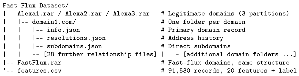
The repository holds four RAR archives and one CSV file, summarised in

Table 2. Main repository files.

File Name	Size	Content Type	Description
Alexa1.rar	1.97 GB	Legitimate domains	First partition of Alexa top-ranked domains for baseline comparison
Alexa2.rar	2.31 GB	Legitimate domains	Second partition of Alexa top-ranked domains for baseline comparison
Alexa3.rar	2.15 GB	Legitimate domains	Third partition of Alexa top-ranked domains for baseline comparison
FastFlux.rar	2.12 GB	Fast-flux domains	Confirmed fast-flux domains with malicious behavior patterns
features.csv	8.5 MB	Engineered features	Machine-learning-ready dataset with 91,530 records and 20 features

. In each archive, each domain has its own folder, and each folder contains the same set of JSON files, so one parser handles the whole collection.

2.1. Repository Structure

Figure 1 shows the layout. Each archive expands to one folder per domain, and each domain folder holds one primary record plus one file per VirusTotal relationship.

2.2. Record Content

The response structure in every JSON file matches the VirusTotal API [26]: it includes a count, an array of data objects, each with the attribute set for that relationship, and self-referential links for paging. Since no reshaping occurred, code previously written for the API can read the files without changes. Timestamps are Unix epoch integers, addresses are dotted quads, ASNs are integers, and country codes follow ISO 3166-1 alpha-2 [27]. The analysis verdicts retain the categories originally returned by the scanning engines, so that the same category has the same meaning on both sides of the collection.

Table 3. Relationship files in a domain folder.

Relationship	Feature Derived	What the Records Themselves Support
Resolutions	Number of IPs, IPs without ASN, ASNs, Countries, Cities, and all three ratios	Address history with per-resolution dates and analysis statistics. The central file for fast-flux work
Subdomains	Number of Sub-Domains	Direct subdomains only, each with its own DNS history, WHOIS, certificate, and analysis records
Siblings	Number of Siblings	Names sharing an immediate parent; exposes the rest of a bulk-registered batch
Parent, Immediate Parent	Number of Parent/Immediate Parent	Separates registered domains from subdomains of one; carries the parent’s creation date and verdicts
Communicating files	Number of Communicated Files	Samples observed contacting the domain, with hashes, submission dates, and per-engine verdicts. Groups domains by the malware that reached them
Referrer files	Number of Referrer Files	Samples containing the domain as a literal string but not observed contacting it. Weaker evidence than a connection, and the two counts diverge sharply between classes
Historical SSL certificates	Number of Historical SSL Certificates	Issuer, subject, validity window and first-seen date. The windows show how long infrastructure stayed in place
Historical WHOIS	Number of Historical WHOIS	Registration snapshots with registrar, abuse contact and name servers; consecutive snapshots differ where ownership changed
Comments, related comments	None	Sparse free-text notes; occasionally name a campaign or malware family

lists the relationships, the feature each contributes, and what the underlying records support beyond that feature. IP address folders carry the same relationships in the same format, minus subdomains, siblings, parent, and immediate parent, which do not apply to an address.

2.3. Feature Dataset

Each feature is a direct count, ratio, or string property of the source JSON; nothing is smoothed, imputed, or normalized, and you can check any value by opening the relevant domain folder and counting the entries. Since the same level of traceability applies, it is easy to include features that we did not compute. The 20 features listed in features.csv are described in

Table 4. Description of the engineered features distributed in features.csv.

Feature Name	Data Type	Value Range	Description	Category
Domain	String	Variable length	Domain name identifier	Identifier
Number of IPs	Integer	1–440+	Count of associated IP addresses	Network connectivity
Number of IPs without ASN	Integer	0–N	Count of IPs lacking ASN information	Network connectivity
Number of ASNs	Integer	2–194+	Count of unique autonomous system numbers	Network connectivity
Number of Countries	Integer	1–N	Count of countries hosting domain IPs	Geographic distribution
Number of Cities	Integer	1–N	Count of cities hosting domain IPs	Geographic distribution
IPs to ASNs Ratio	Float	1.0–N	Ratio of IP addresses to ASN count	Infrastructure metrics
IPs to Countries Ratio	Float	1.0–N	Ratio of IP addresses to country count	Infrastructure metrics
IPs to Cities Ratio	Float	1.0–N	Ratio of IP addresses to city count	Infrastructure metrics
Domain Length	Integer	4–244	Character count of the domain name	Domain characteristics
Domain Entropy	Float	2.0–4.0+	Information entropy of a domain name	Domain characteristics
TLD Type	Integer	1–N	Top-level domain type classification	Domain characteristics
Has Private Owner	Boolean	True/False	Private WHOIS registration indicator	Registration characteristics
Number of Communicated Files	Integer	0–N	Count of communicating files	Behavioral analysis
Number of Historical SSL Certificates	Integer	0–N	Count of SSL certificate history records	Historical analysis
Number of Historical WHOIS	Integer	0–N	Count of WHOIS history records	Historical analysis
Number of Parent/ Immediate Parent	Integer	0–N	Count of parent domain relationships	Relationship analysis
Number of Referrer Files	Integer	0–N	Count of referrer files	Traffic analysis
Number of Sub-Domains	Integer	0–N	Count of discovered subdomains	Infrastructure analysis
Number of Siblings	Integer	0–N	Count of sibling domains	Relationship analysis
Label	Integer	0 or 1	Classification label (0 = legitimate, 1 = fast-flux)	Target variable

.

3. Methods

The collection pipeline is the one developed for PASSVM [5], extended with a VirusTotal expansion step and run at a larger scale.

Table 5. Collection pipeline: the seven stages used to build the dataset, where # is the stage number.

#	Stage	What Was Done
1	Seed the malicious side	80 confirmed fast-flux domains taken from published work [3,4,5] and from tweets reporting newly discovered domains
2	Active resolution	Each unique name resolved repeatedly with the Linux dig utility for just over two months; addresses read from the DNS response messages
3	VirusTotal expansion	Every observed address queried for the domains it had resolved to since April 2018, with the dates of those resolutions. The expansion yields 67,606 fast-flux domains
4	Seed the benign side	Alexa top-ranked list resolved the same way; we kept only domains returning five or more addresses, since a single A-record domain cannot exhibit flux and would make the comparison trivial. The expansion yields 23,924 legitimate domains
5	Relationship retrieval	For every domain and address, all VirusTotal relationships in Table 3 retrieved and stored unmodified
6	Network enrichment	Censys queried through its API for distinct ports, addresses, countries and cities; ASN and country attribution per address taken from a free IP geolocation database
7	Feature computation	The 20 features in Table 4 computed from the stored JSON, producing 91,530 labelled records

lists its stages.

Two points about labeling. First, the fast-flux label is inherited: a domain enters the malicious half because it was served by an address that a confirmed fast-flux domain also resolved to. Shared hosting infrastructure is the labeling criterion. That is appropriate for the threat model in Section 1.1, but it is not the same as per-domain manual confirmation. Second, the benign label is Alexa membership, which is a popularity signal rather than a guarantee of cleanliness. Both choices are visible in the raw records and can be revisited by anyone who wants a stricter criterion.

Geolocation is used only at country and ASN granularity. Free geolocation databases are unreliable at city level, so city counts are reported for completeness and are not relied on where precision matters.

4. User Notes

4.1. Intended Use

The dataset supports three tasks. They differ in their inputs and in what a result means.

Task 1: fast-flux detection: Binary classification of a domain from features.csv. This is the task the baseline in Section 4.5 performs, and the default for comparing detectors. The Domain column is an identifier and has to be dropped before training; leaving it in leaks the label through the name itself.

Task 2: separating flux from legitimate multi-homing: The hard case for any fast-flux detector is a legitimate domain served from many addresses in many countries, which is what a CDN looks like [1]. Restricting the benign half to its upper decile by Number of ASNs produces a hard-negative subset. Scoring a detector on the full set and on that subset separates detectors that have learned flux from detectors that have learned multi-homing. This is where our baseline is weakest, and where a new method has the most room to show its value.

Task 3: infrastructure analysis: No labels and no classifier. The raw archives support address reuse across domains and campaigns, registrar and name-server concentration, certificate validity windows as a proxy for how long infrastructure survives, and grouping of domains by the malware samples observed contacting them.

4.2. Reference Evaluation Protocol

Results on this dataset are comparable only if they are produced the same way. We recommend the following and used it for the baseline.

• Splitting: Five-fold stratified cross-validation over the 91,530 records.
• Leakage control: Group folds by registered parent domain. Subdomains of one parent share hosting and registration properties, so splitting them across folds inflates every metric.
• Excluded columns: Drop Domain. Train on the 19 numeric and categorical features and predict Label.
• Metrics: Report per-class true positive rate, false positive rate, precision, recall, and F1, and report the false positive rate at a fixed true positive rate of 0.95. Accuracy may be quoted, but only next to the per-class rates: the classes are unbalanced at roughly three to one, so a classifier that labels everything fast flux already scores 73.9%.
• Hard negatives: Repeat the evaluation on the Task 2 subset and report both numbers.

4.3. Feature Distributions

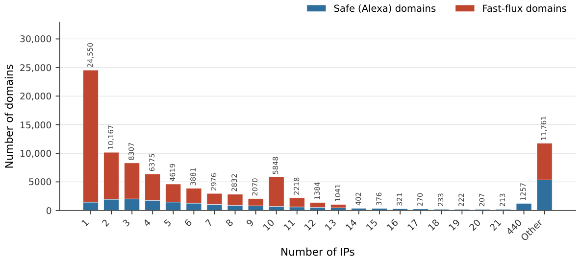
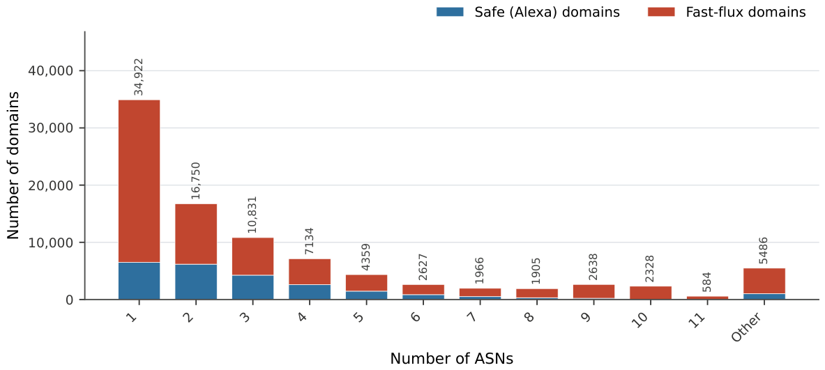
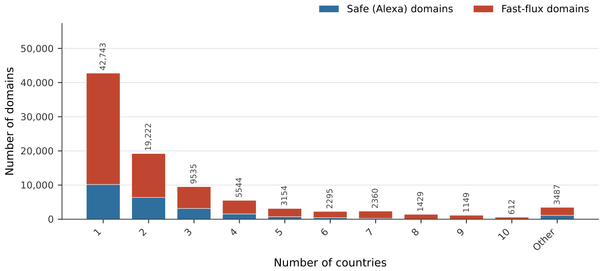
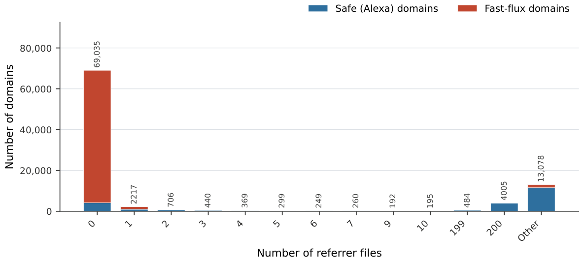
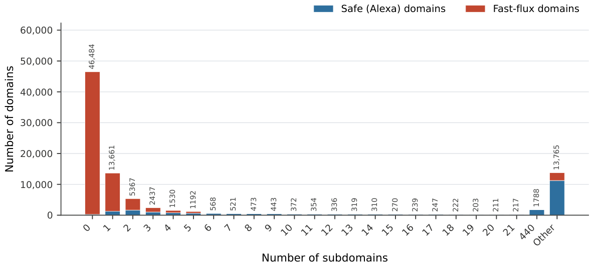
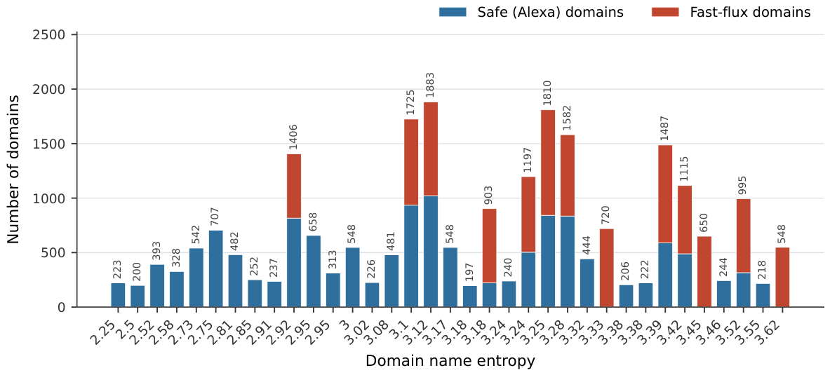
Figure 2, Figure 3, Figure 4, Figure 5, Figure 6 and Figure 7 show six representative features, as stacked counts by category with the two labels distinguished. We collect categories with few members into an “Other” bar, applied separately to each class, so a category retained for one class but not the other reads as zero for the latter; counts for those categories are lower bounds.

Table 6. What the feature distributions show.

Feature	Shape of the Distribution	Figure
Number of IPs	Flux shows up here first: the benign half concentrates in the low categories while the fast-flux half spreads across the range and carries most of the “Other” bar	Figure 2
Number of ASNs	Hosting spread across unrelated autonomous systems, the defining shape of fast flux. The classes separate clearly, though the forest leans more on the relationship counts	Figure 3
Number of Countries	Separates the classes only in combination with the ASN count, because legitimate CDNs also span countries	Figure 4
Number of Referrer Files	Diverges sharply between classes and ranks second in importance	Figure 5
Number of Sub-Domains	Ranks first in importance; bulk-registered infrastructure shows a characteristic profile	Figure 6
Domain Entropy	Often treated as a strong signal for generated names, but the two classes overlap heavily here	Figure 7
IPs without ASN, and the IPs-to-ASNs, IPs-to-Countries and IPs-to-Cities ratios	Ratio features compress the same hosting-spread signal and are correlated with it	Figures S1–S4
Number of Cities	Follows the country distribution, at lower reliability	Figure S5
Domain Length, TLD Type, Has Private Owner	Name and registration properties; weak separators on their own	Figures S6–S8
Communicated Files, Historical SSL Certificates, Historical WHOIS, Parent/Immediate Parent, Siblings	Behavioral and relationship counts; the parent count is close to binary, which is what makes it useful	Figures S9–S13

summarises what every feature distribution shows.

4.4. Structure of the Feature Space

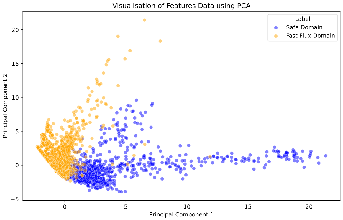
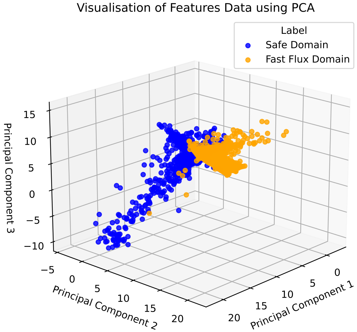
Principal component analysis reduces the 19 numeric features to orthogonal components ordered by explained variance [28], computed here by singular value decomposition. Plotting the leading components before choosing a classifier shows whether the classes are separable and where the hard cases lie.

Figure 8 plots a 10% sample on the first two components, and Figure 9 adds the third. Most separation occurs along the first component. Fast-flux domains crowd into its low end while the Alexa domains spread out along it, with a dense overlap near the origin. The second and third components do far less work and leave the classes largely mixed; those two projections are in the supplementary figure pack. The separation the random forest finds is therefore not one a human eye picks out of a scatter plot.

4.5. Baseline Results

A random forest consisting of 200 trees was trained in scikit-learn [29] using the file features.csv according to the protocol described in Section 4.2 and achieved correct classification of 96.0% of the 91,530 records. The fact that the classes are unbalanced means that the rates for each class listed in

Table 7. Detailed accuracy by class for the random forest baseline.

Class	TP Rate	FP Rate	Precision	Recall	F1 Score
Safe	0.9017	0.0193	0.9428	0.9017	0.9218
Fast flux	0.9807	0.0983	0.9658	0.9807	0.9731

are more important than that percentage.

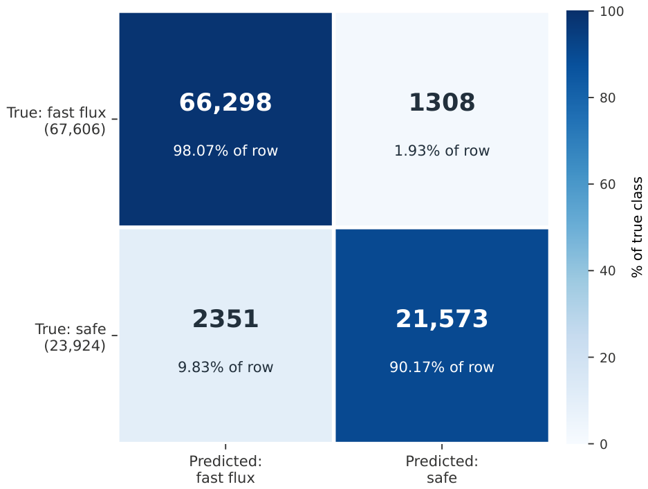
The true and false positives and negatives are obtained from the confusion matrix shown in Figure 10, upon which the standard rates are based. The true and false positive rates are given by Equations (1) and (2), accuracy is provided by Equation (3), precision is given by Equation (4), and the F1 score, which is the harmonic mean of precision and recall, is given by Equation (5). Pay attention to precision when a false positive means blocking a legitimate site.

$$T{P}_{Rate}={\displaystyle \frac{TP}{TP+FN}}$$

(1)

$$F{P}_{Rate}={\displaystyle \frac{FP}{TN+FP}}$$

(2)

$$Accuracy={\displaystyle \frac{TP+TN}{TP+TN+FP+FN}}$$

(3)

$$Precision={\displaystyle \frac{TP}{FP+TP}}$$

(4)

$$F{1}_{score}={\displaystyle \frac{2}{{recall}^{-1}+{Precision}^{-1}}}$$

(5)

Of the 67,606 fast-flux records, 66,298 are caught, and 1308 are missed. Of the 23,924 benign records, 21,573 are classified correctly, and 2351 are flagged as fast flux. That second number is the one to argue about. A 10% false-positive rate on legitimate domains is tolerable in an offline study but expensive in a live blocking pipeline, and it is where a method evaluated on this dataset has the most room to improve on the baseline.

4.6. Feature Importance

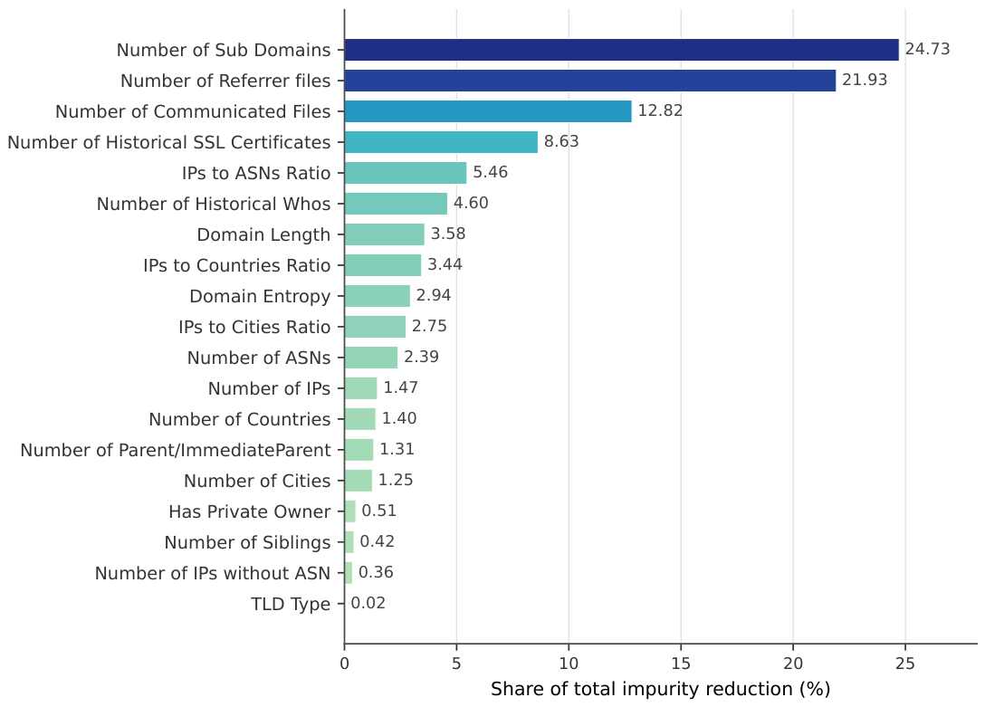
The random forest records how much each feature reduced impurity during splits, averaged across all trees. As Figure 11 illustrates, the ranking is as follows: the number of subdomains is first with 24.7% of the total impurity reduction, then the number of referrer files at 21.9% and the number of communicated files at 12.8%; together these three make up almost 60% of the decision. The hosting-spread features rank lower than one might expect given the fast-flux framing: the IP-to-ASN ratio reaches 5.5%, and the raw ASN count is only 2.4%. Although the spread across autonomous systems separates the classes, as Figure 3 shows, the forest finds it cheaper to split on relationship and reputation counts. These counts are also most affected by how much of a domain VirusTotal happened to see. TLD type and the number of siblings contribute almost nothing, and domain entropy—although often regarded as a strong indicator of algorithmically generated domains—lies in the lower half. Test both results on other data before generalizing.

4.7. Reading the Baseline Against Published Results

Table 8. Reported detection results and the data behind them.

Work	Method	Reported	Evaluation Data
Al-Duwairi et al. [5]	SVM (RBF kernel)	99.557% acc.	Authors’ own collection, not released
Nagunwa et al. [18]	Supervised ML, 56 features	98.42% acc.	Authors’ own collection, not released
Ayo et al. [7]	Genetic rules with kNN	>99% acc.	Authors’ own botnet domains, not released
Silveira et al. [22]	Semi-supervised ensemble	0.962 AUC	TLD registry data, not released
This baseline	Random forest, 19 features	96.0% acc.	features.csv, public, protocol in Section 4.2

lists accuracies reported by recent fast-flux and malicious-domain detectors. The baseline here is lower than most of them, and the comparison is not meaningful in the direction it appears to run.

Each of the first four numbers was produced on a different set of domains, with a different benign population, a different class balance, and in most cases a different definition of what counts as fast flux. None of them can be reproduced, and none can be traded off against another. The baseline reported here makes no claim to beat them. Its purpose is to fix a reference point that anyone can reproduce and improve on, and to make the false positive rate on legitimate domains visible, which is the number a protective DNS operator has to live with [1] and which a headline accuracy conceals.

4.8. Limitations

The VirusTotal API provides a maximum of 40 items per request for a relationship; when a relationship contains more than that, we made up to 10 requests and then stopped, ensuring that a domain is associated with at most 400 resolutions. Domains at the top end of the range are right-censored, and any figure relating to the number of addresses per domain should be interpreted with that upper limit in mind.

The account refers to a specific time period; the DNS component operated for two months, and the VirusTotal resolution history goes back to April 2018, so the hosting and registration behavior recorded here applies to that period, not the present day. We provide the feature definitions and collection code so you can refresh the data using up-to-date information.

Alexa’s ranking service has since been retired, so we can’t regenerate the benign list from the same source. The archives preserve the exact domains used, so the benign half remains reproducible.

The two halves are unbalanced at roughly three fast-flux records to one benign record, and the labeling is inherited rather than individually confirmed. TTL values are not recorded, so this benchmark excludes classical TTL-based detectors.

References

1. National Security Agency; Cybersecurity and Infrastructure Security Agency; Federal Bureau of Investigation; Australian Signals Directorate’s Australian Cyber Security Centre; Canadian Centre for Cyber Security; New Zealand National Cyber Security Centre. Fast Flux: A National Security Threat. Joint Cybersecurity Advisory AA25-093A. 2025. Available online: https://www.cisa.gov/news-events/cybersecurity-advisories/aa25-093a (accessed on 1 September 2026).
2. MITRE. Dynamic Resolution: Fast Flux DNS (T1568.001) and Detection Strategy DET0485. MITRE ATT&CK Enterprise Matrix, 2025. Available online: https://attack.mitre.org/detectionstrategies/DET0485/ (accessed on 1 September 2026).
3. Zang, X.D.; Gong, J.; Mo, S.H.; Jakalan, A.; Ding, D.L. Identifying Fast-Flux Botnet with AGD Names at the Upper DNS Hierarchy. IEEE Access 2018, 6, 69713–69727. [Google Scholar] [CrossRef] [Scilit]
4. Lombardo, P.; Saeli, S.; Bisio, F.; Bernardi, D.; Massa, D. Fast Flux Service Network Detection via Data Mining on Passive DNS Traffic. In Proceedings of the Information Security (ISC 2018), Guildford, UK, 9–12 September 2018; Volume 11060, pp. 463–480. [Google Scholar] [CrossRef] [Scilit]
5. Al-Duwairi, B.; Jarrah, M.; Shatnawi, A.S. PASSVM: A Highly Accurate Fast Flux Detection System. Comput. Secur. 2021, 110, 102431. [Google Scholar] [CrossRef] [Scilit]
6. Zhu, Z.; Lu, G.; Chen, Y. Botnet research survey. In Proceedings of the 2008 32nd Annual IEEE International Computer Software and Applications Conference, Turku, Finland, 28 July–1 August 2008; pp. 967–972. [Google Scholar]
7. Ayo, F.E.; Awotunde, J.B.; Folorunso, S.O.; Adigun, M.O.; Ajagbe, S.A. A genomic rule-based KNN model for fast flux botnet detection. Egypt. Inform. J. 2023, 24, 313–325. [Google Scholar] [CrossRef] [Scilit]
8. Zeidanloo, H.R.; Shooshtari, M.J.Z. A taxonomy of botnet detection techniques. In Proceedings of the 2010 3rd International Conference on Computer Science and Information Technology, Chengdu, China, 9–11 July 2010; pp. 158–162. [Google Scholar]
9. Provos, N. A virtual honeypot framework. In Proceedings of the USENIX Security Symposium, San Diego, CA, USA, 9–13 August 2004; pp. 1–14. [Google Scholar]
10. Vrable, M.; Ma, J.; Chen, J.; Moore, D.; Vandekieft, E.; Snoeren, A.C.; Voelker, G.M.; Savage, S. Scalability, fidelity, and containment in the potemkin virtual honeyfarm. SIGOPS Oper. Syst. Rev. 2005, 39, 148–162. [Google Scholar] [CrossRef] [Scilit]
11. Bajtos, T.; Sokol, P. Virtual honeypots and detection of telnet botnets. In Proceedings of the Central European Cybersecurity Conference, Ljubljana, Slovenia, 15–16 November 2018; pp. 1–6. [Google Scholar]
12. Gu, G.; Porras, P.A. Bothunter: Detecting malware infection through IDS-driven dialog correlation. In Proceedings of the USENIX Security Symposium, Boston, MA, USA, 6–10 August 2007; pp. 1–16. [Google Scholar]
13. Chen, T.; Zhou, G.; Liu, Z.; Jing, T. A novel ensemble anomaly-based approach for command and control channel detection. In Proceedings of the 2020 4th International Conference on Cryptography, Security and Privacy, Nanjing, China, 10–12 January 2020; pp. 74–78. [Google Scholar]
14. Martinez-Bea, S.; Castillo-Perez, S.; Garcia-Alfaro, J. Real-time malicious fast-flux detection using DNS and bot-related features. In Proceedings of the 2013 Eleventh Annual Conference on Privacy, Security and Trust, Tarragona, Spain, 10–12 July 2013; pp. 369–372. [Google Scholar]
15. Alieyan, K.; Almomani, A.; Anbar, M.; Alauthman, M.; Abdullah, R.; Gupta, B.B. DNS rule-based schema for botnet detection. Enterp. Inf. Syst. 2021, 15, 545–564. [Google Scholar] [CrossRef] [Scilit]
16. Ibrahim, W.N.H.; Anuar, S.; Selamat, A.; Krejcar, O.; Crespo, R.G.; Herrera-Viedma, E.; Fujita, H. Multilayer framework for botnet detection using machine learning algorithms. IEEE Access 2021, 9, 48753–48768. [Google Scholar] [CrossRef] [Scilit]
17. Ramachandran, A.; Feamster, N.; Dagon, D. Revealing botnet membership using DNSBL counter-intelligence. In Proceedings of the 2nd Workshop on Steps to Reducing Unwanted Traffic on the Internet (SRUTI ’06), San Jose, CA, USA, 7 July 2006; pp. 49–54. [Google Scholar]
18. Nagunwa, T.; Kearney, P.; Fouad, S. A machine learning approach for detecting fast flux phishing hostnames. J. Inf. Secur. Appl. 2022, 65, 103125. [Google Scholar] [CrossRef] [Scilit]
19. Goldberg, D.E.; Holland, J.H. Genetic algorithms and machine learning. Mach. Learn. 1988, 3, 95–99. [Google Scholar] [CrossRef] [Scilit]
20. Lin, H.T.; Lin, Y.Y.; Chiang, J.W. Genetic-based Real-time Fast-Flux Service Networks Detection. Comput. Netw. 2013, 57, 501–513. [Google Scholar] [CrossRef] [Scilit]
21. Hosseini, S.; Nezhad, A.E.; Seilani, H. Botnet detection using negative selection algorithm, convolution neural network and classification methods. Evol. Syst. 2022, 13, 101–115. [Google Scholar] [CrossRef] [Scilit]
22. Silveira, M.R.; Cansian, A.M.; Kobayashi, H.K. Semi-supervised approach for detecting malicious domains in TLDs in their first query. Int. J. Inf. Secur. 2025, 24, 80. [Google Scholar] [CrossRef] [Scilit]
23. Shafi, M.; Lashkari, A.H.; Mohanty, H. Unveiling malicious DNS behavior profiling and generating benchmark dataset through application layer traffic analysis. Comput. Electr. Eng. 2024, 118, 109436. [Google Scholar] [CrossRef] [Scilit]
24. Chandra, S.; Singh, M.; Gangopadhyaya, M.; Chakraborty, S.; Chowdhury, I. Fast Flux Network-Based Detection of Malicious DNS Domains. In Proceedings of the International Conference on Computational Intelligence, Data Science and Cloud Computing (IEM-ICDC 2025), Kolkata, India, 11–12 April 2025; Volume 1541. [Google Scholar] [CrossRef] [Scilit]
25. Mahdavifar, S.; Maleki, N.; Lashkari, A.H.; Broda, M.; Razavi, A.H. Classifying Malicious Domains using DNS Traffic Analysis. In Proceedings of the 2021 IEEE Intl Conf on Dependable, Autonomic and Secure Computing (DASC), Online, 25–28 October 2021. [Google Scholar]
26. VirusTotal. VirusTotal API v3: Domain Objects and Relationships. 2024. Available online: https://docs.virustotal.com/reference/domains-object (accessed on 1 September 2024).
27. ISO 3166-1:2020; Codes for the Representation of Names of Countries and Their Subdivisions—Part 1: Country Code. International Organization for Standardization: Geneva, Switzerland, 2020.
28. Maćkiewicz, A.; Ratajczak, W. Principal components analysis (PCA). Comput. Geosci. 1993, 19, 303–342. [Google Scholar] [CrossRef] [Scilit]
29. Pedregosa, F.; Varoquaux, G.; Gramfort, A.; Michel, V.; Thirion, B.; Grisel, O.; Blondel, M.; Prettenhofer, P.; Weiss, R.; Dubourg, V.; et al. Scikit-learn: Machine Learning in Python. J. Mach. Learn. Res. 2011, 12, 2825–2830. [Google Scholar]
Figure 1. Structure of the published repository.
Data 11 00244 g001
Figure 2. Number of IPs by category, split by label. Categories with few members are grouped as “Other”.
Data 11 00244 g002
Figure 3. Number of ASNs by category, split by label.
Data 11 00244 g003
Figure 4. Number of countries by category, split by label.
Data 11 00244 g004
Figure 5. Number of referrer files by category, split by label.
Data 11 00244 g005
Figure 6. Number of subdomains by category, split by label.
Data 11 00244 g006
Figure 7. Domain Entropy by category, split by label. Entropy takes several hundred distinct values, so the “Other” group holds 67,598 domains (73.9% of the corpus) and is omitted from the plot to keep the remaining categories on a readable scale.
Data 11 00244 g007
Figure 8. First and second principal components, coloured by label (10% sample).
Data 11 00244 g008
Figure 9. First three principal components, coloured by label (10% sample).
Data 11 00244 g009
Figure 10. Random forest confusion matrix.
Data 11 00244 g010
Figure 11. Random forest feature importance.
Data 11 00244 g011