Comparison of Trigonometric Distribution Families Under Classical and Bayesian Approaches

Abstract

This study aims to compare the performance of trigonometric families of distributions, sine-G, cosine-G, and tangent-G, using the inverse Weibull distribution as a baseline, and to guide model selection for six different data structures. Six real datasets with varying distributional characteristics, including right-skewed, left-skewed, and symmetric patterns, were used for comparison and analysis. Model performance was evaluated using both classical and Bayesian model comparison approaches. Across all six datasets, the sine-G family consistently outperformed the cosine-G and tangent-G families using inverse Weibull as a base distribution. The trigonometric families showed strong suitability for right-skewed data but demonstrated limited effectiveness for left-skewed and symmetric datasets. For the Sin-IW model, strong goodness-of-fit performance was observed across datasets with different skewness patterns. For right-skewed datasets (Datasets 1 and 3), the model produced AIC values of 437.4989 and 118.6208 with corresponding KS p-values of 0.9359 and 0.8771. For the symmetric dataset (Dataset 2), the AIC and KS p-value were 118.0071 and 0.6631, respectively. For moderately left-skewed (Dataset 4) and left-skewed data (Dataset 6), the AIC values were 128.1826 and 112.0453 with KS p-values of 0.3138 and 0.0774. For the extremely right-skewed dataset (Dataset 5), the model achieved an AIC of 68.5246 and a KS p-value of 0.9960. Bayesian model comparison further supported the superiority of the Sin-IW model. For Dataset 1, the WAIC values were 474.40 (Sin-IW), 474.60 (Cos-IW), and 493.50 (Tan-IW), while for Dataset 6, the WAIC values were 200.60 (Sin-IW), 207.90 (Cos-IW), and 209.70 (Tan-IW), confirming that Sin-IW demonstrated a good fit for classical and Bayesian inference. These results highlight the robustness of the Sin-G family among trigonometric distributions and offer practical insights for selecting appropriate models when analyzing data with diverse distributional features.

1. Introduction

Probability distributions are the foundation of inferential statistics, as they form the basis for most statistical models used in real-world data analysis. With advancements in modern technology, data generation and collection processes have become faster and more convenient, leading to a wide variety of data scenarios. However, existing probability distributions often lack the flexibility to adequately model these diverse data structures, necessitating the development of new probability distributions to address such complexities. A common strategy for addressing this challenge is to extend existing probability distributions by adding parameters. Trigonometric transformations constitute one of the earliest approaches for generating new distribution families and often provide simpler models with better fits to real-world data [1]. Despite the development of numerous trigonometric families of distributions for applications ranging from circular data [1,2] to extreme-value analysis [3,4], their comprehensive comparison remains unexplored. Such a comparison is essential for practitioners seeking to identify the most suitable family for a given data scenario.

Originating in the nineteenth century [5], trigonometric families of distributions were initially developed to model circular data, such as wind directions, animal movement patterns, and cyclical environmental phenomena [1,2]. Their flexibility has since broadened their applicability to the analysis of datasets involving extreme values [3,4]. The introduction of the SS transformation by Kumar et al. [6], followed by Souza’s development of the Sin-G [7], Cos-G [8], and Tan-G [9] families, has renewed interest in and accelerated the growth of trigonometric families of distributions in recent decades. Subsequently, several distribution families were introduced following the SS transformation’s introduction. Some of the notable contributions include a new class of Sin-G distribution [10], a new class of Tan-G [11], Sin $\pi$-power odd-G FD [12], Cos $\pi$-power odd-G FD [13], and a new Sin family of generalized distributions [14]. Further developments include a new Sin-G family of distributions [15], a Sin Topp-Leone-G family of distributions [16], a Sin Kumaraswamy-G family of distributions [17], a Sin generalized family of distributions [18], and  a transmuted Sin-G family of distributions [19]. Other notable advancements include the following, beyond the Sin-G family: the transformed Sin-G family of distributions [20], the Sin inverse Lomax-generated family of distributions [21], the Sin F-Loss family of distributions [22], the Sin Type II Topp-Leone-G family of distributions [23], the Sin modified power-generated family of distributions [24], and the Marshall–Olkin Sin–G family of distributions [25]. Further developments include the arc-tangent-G family of distributions [26], the weighted Cos-G family of distributions [27], and the family of distributions generated using the tangent function [28].

Unlike the early development of trigonometric models, which primarily focused on addressing challenges in circular and extreme-value data, modern advancements extend far beyond these applications. Recent development of trigonometric models is recognized for their flexibility in capturing a wide variety of data shapes, including increasing, decreasing, bathtub, inverted bathtub, increasing–decreasing, constant, and skewed patterns. For example, the Sine modified Lindley distribution developed by Tomy and Chesneau [29] is useful for modeling lifetime data exhibiting right skewness, leptokurtic, and increasing or reverse bathtub-shaped hazard rates. Similarly, Muhammad et al. [30] introduced the exponentiated Sin-G family of distributions for modeling diverse hazard shapes, including increasing, decreasing, and bathtub forms. Likewise, Mohammad and Cooray [5] proposed a trigonometric family tailored for highly skewed actuarial data.

As discussed earlier, several trigonometric families of distributions have been proposed in the literature and have proven capable of modeling a wide variety of data situations. However, it is unclear whether these families are universally applicable to all types of data scenarios. In real-world applications, practitioners often encounter diverse data characteristics, such as right-skewed data, like annual flood discharge data [31], symmetric datasets, like carbon fiber strength [32], right-skewed data, such as the time to failure of non-repairable items [33], and left-skewed data, like the failure time of turbochargers [34]. Given this variety of data distributions, the following question arises: are all of the presented families of trigonometric distributions equally suitable for fitting these different types of data? If not, when should each type of trigonometric distribution family be applied? This remains an open question. In the applied world of statistics, end users are typically less interested in abstract mathematical derivations of probability distributions and their theoretical properties. Instead, they require practical guidance to select appropriate methods for their applied research. Consequently, applied statisticians have an additional responsibility to communicate essential, application-oriented information to end users. To the best of our knowledge, no existing studies systematically compare trigonometric families of distributions across diverse data shapes, such as right-skewed, left-skewed, and symmetric distributions. To address this gap, the present study provides a comprehensive, application-oriented comparison of inverse Weibull (IW) based trigonometric family distributions across diverse real-world datasets using both classical and Bayesian inferential frameworks. Through this comparison, end users can gain insights into the relative behavior of different trigonometric distributions, which may inform the selection of distributions suitable for their data. The validity of the proposed models was evaluated using Monte Carlo simulations, and their performance was compared across six real-world data scenarios using classical approaches. Finally, the three models were fitted to two distinct datasets within a Bayesian approach, and a comparative analysis was conducted to select the model that provided the best fit under each data scenario.

The outline of this paper is as follows: In Section 2, the development of trigonometric models based on three trigonometric families, using the IW distribution as the base, is presented. Section 3 discusses the classical approach to parameter estimation for all presented models. In Section 4, a simulation study is provided. Section 5 presents the application of the proposed models to six different real-world data scenarios and compares the performance of all three models. In Section 6, parameter estimation for the presented models is performed using Bayesian estimation across two distinct data scenarios. Finally, Section 7 offers a summary and conclusion.

2. Specific Trigonometric Models

To explore the Sin-G, Cos-G, and Tan-G families of distributions, we developed trigonometric models associated with each. The IW distribution was selected as the base for defining these models due to its ability to provide elegant and mathematically simple forms for the CDF and probability density function (PDF) of the resulting distributions. It is also well-suited for modeling right-skewed and heavy-tailed lifetime data and is widely used in reliability and survival analysis. In addition, most trigonometric-based models were typically defined using the inverse type base models, such as the IW distribution. Hence, we used the IW distribution as the base distribution, following Refs. [35,36] and expressed it as follows:

$$W\left(x\right)=\exp (-\theta x^{-\delta });x>0,(\theta ,\delta )>0.$$

(1)

$$w\left(x\right)=\delta \theta \exp (-\theta x^{-\delta })x^{-(\delta +1)}.$$

(2)

2.1. Sine Inverse Weibull (Sin-IW) Distribution

The CDF of Sin-G family, proposed by [7], is defined as:

$$F(x;\xi )={\displaystyle \underset{0}{\overset{{\displaystyle \frac{\pi }{2}}G(x;\xi )}{\int }}}\cos \left(t\right),dt=\sin \left({\displaystyle \frac{\pi }{2}}G(x;\xi )\right),x\in \mathbb{R}.$$

(3)

where $G(x;\xi )$ is the CDF of any parent distribution and $\xi$ is the vector of parameters of the parent distribution.

By substituting Equation (1) as the base distribution in the Sin-G family (Equation (3)), the CDF of the Sin-IW distribution can be expressed as follows:

$$\begin{array}{cc}\hfill F\left(x\right)& =\sin \left({\displaystyle \frac{\pi }{2}}\exp (-\theta x^{-\delta })\right);x>0,(\theta ,\delta )>0,\hfill \\ \hfill & =\sin \left({\displaystyle \frac{\pi }{2}}Z\right),\hfill \end{array}$$

(4)

where $Z=\exp (-\theta x^{-\delta })$. Using Equation (4), the PDF of the Sin-IW distribution is derived as

$$\begin{array}{cc}\hfill f\left(x\right)=& {\displaystyle \frac{\pi }{2}}\theta \delta x^{-(\delta +1)}Z\cos \left({\displaystyle \frac{\pi }{2}}Z\right);x>0.\hfill \end{array}$$

(5)

The survival function of the Sin-IW distribution is expressed as

$$S\left(x\right)=1-\sin \left({\displaystyle \frac{\pi }{2}}Z\right),x>0.$$

The hazard rate function (HRF) is given by

$$\begin{array}{c}\hfill h\left(x\right)={\displaystyle \frac{\frac{\pi }{2}\theta \delta x^{-(\delta +1)}Z\cos \left(\frac{\pi }{2}Z\right)}{1-\sin \left(\frac{\pi }{2}Z\right)}}.\end{array}$$

(6)

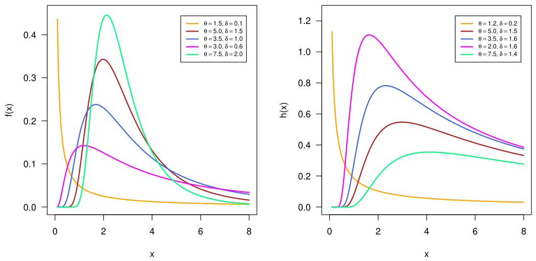
Figure 1 illustrates the flexibility of the Sin-IW distribution for different values of the parameters $\theta$ and $\delta$. The PDF can exhibit either a decreasing or a unimodal right-skewed shape. Smaller values of $\delta$ produce densities concentrated near the origin, whereas larger values generate more pronounced unimodal curves. The HRF shows both decreasing and upside-down bathtub shapes, with the overall pattern and peak location influenced by the choices of $\theta$ and $\delta$. These results demonstrate the ability of the Sin-IW distribution to accommodate a wide range of lifetime data behaviors.

The quantile function (QF) for the Sin-IW distribution can be expressed as

$$Q_X\left(p\right)={\left[-{\displaystyle \frac{1}{\theta }}\log \left({\displaystyle \frac{2}{\pi }}{\sin }^{-1}\left(p\right)\right)\right]}^{-{\displaystyle \frac{1}{\delta }}};p\in (0,1),$$

(7)

where p is a random variable that follows the uniform distribution on the interval (0, 1).

2.2. Cosine Inverse Weibull (Cos-IW)

The CDF of Cos-G family, proposed by [8], is defined as:

$$F(x;\xi )=-{\displaystyle \underset{0}{\overset{{\displaystyle \frac{\pi }{2}}\left(G(x;\xi )\right)}{\int }}}\sin \left(t\right)dt=1-\cos \left[{\displaystyle \frac{\pi }{2}}G(x;\xi )\right];x\in \Re .$$

(8)

where $G(x;\xi )$ is the CDF of any parent distribution and $\xi$ is the vector of parameters of the parent distribution.

By substituting Equation (1) as the base distribution in the Cos-G family (Equation (8)), the CDF of the Cos-IW distribution is obtained as

$$F\left(x\right)=1-\cos \left({\displaystyle \frac{\pi }{2}}Z\right);x>0.$$

(9)

Using Equation (9), the PDF of the Cos-IW distribution is derived as

$$\begin{array}{cc}\hfill f\left(x\right)=& {\displaystyle \frac{\pi }{2}}\theta \delta x^{-(\delta +1)}Z\sin \left({\displaystyle \frac{\pi }{2}}Z\right);x>0.\hfill \end{array}$$

(10)

The hazard function of Cos-IW can be expressed as

$$\begin{array}{cc}\hfill & h\left(x\right)={\displaystyle \frac{\pi }{2}}\theta \delta x^{-(\delta +1)}Z\sin \left({\displaystyle \frac{\pi }{2}}Z\right){\left[\cos \left({\displaystyle \frac{\pi }{2}}Z\right)\right]}^{-1}.\hfill \end{array}$$

(11)

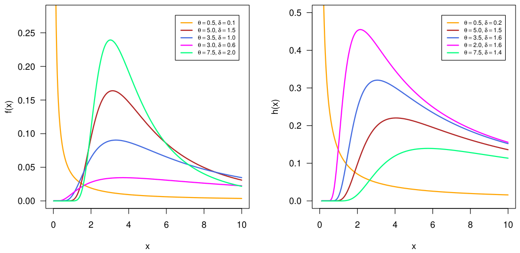
The various shapes of the PDF and HRF of the Cos-IW distribution are illustrated in Figure 2. It is observed that the Cos-IW also has similar shapes of PDF and HRF to those of Sin-IW. The QF of the Cos-IW distribution can be presented as

$$Q_X\left(p\right)={\left[-{\displaystyle \frac{1}{\theta }}\log \left({\displaystyle \frac{2}{\pi }}{\cos }^{-1}(1-p)\right)\right]}^{-{\displaystyle \frac{1}{\delta }}};p\in (0,1).$$

(12)

Some fundamental statistical and mathematical properties of the Cos-IW are included in the Supplementary Materials in Section S2.

2.3. Tangent Inverse Weibull (Tan-IW) Distribution

The CDF of Tan-G family, proposed by [9], is defined as:

$$F(x;\xi )={\displaystyle \underset{0}{\overset{{\displaystyle \frac{\pi }{4}}\left(G(x;\xi )\right)}{\int }}}{\sec }^2\left(t\right)dt=\tan \left[{\displaystyle \frac{\pi }{4}}G(x;\xi )\right];x\in \Re .$$

(13)

where $G(x;\xi )$ is the CDF of any parent distribution and $\xi$ is the vector of parameters of the parent distribution.

By substituting Equation (1) as the base distribution in the Tan-G family defined by [9], the CDF of the tan-IW distribution is obtained as

$$\begin{array}{c}\hfill F\left(x\right)=\tan \left({\displaystyle \frac{\pi }{4}}Z\right);x>0.\end{array}$$

(14)

Using Equation (14), the PDF of the Tan-IW distribution is derived as

$$\begin{array}{cc}\hfill f\left(x\right)=& {\displaystyle \frac{\pi }{4}}\theta \delta x^{-(\delta +1)}Z{\sec }^2\left({\displaystyle \frac{\pi }{4}}Z\right);x>0.\hfill \end{array}$$

(15)

Furthermore, the hazard function of Tan-IW can be presented as

$$\begin{array}{cc}\hfill h\left(x\right)& ={\displaystyle \frac{\pi }{4}}\theta \delta x^{-(\delta +1)}Z{\sec }^2\left({\displaystyle \frac{\pi }{4}}Z\right){\left[1-\tan \left({\displaystyle \frac{\pi }{4}}Z\right)\right]}^{-1};x>0.\hfill \end{array}$$

Similarly, the QF for the Tan-IW distribution can be expressed as

$$Q_X\left(p\right)={\left[-{\displaystyle \frac{1}{\theta }}\log \left({\displaystyle \frac{4}{\pi }}{\tan }^{-1}\left(p\right)\right)\right]}^{-{\displaystyle \frac{1}{\delta }}};p\in (0,1).$$

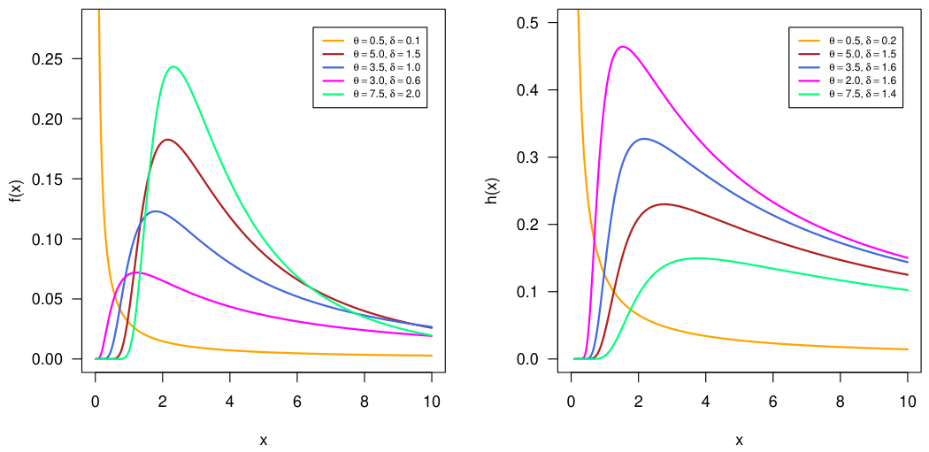
The other distributional properties of the Tan-IW distribution can be obtained as described in Section S2 for Cos-IW of the Supplementary Materials. The possible shapes of the PDF and HRF of the Tan-IW distribution are illustrated in Figure 3. It is observed that the Tan-IW also has similar shapes of PDF and HRF to those of Sin-IW.

3. Classical Approach for Parameter Estimation

The parameters of the model under investigation were estimated using the maximum likelihood estimation (MLE) method. Due to the non-linear nature of the log-likelihood functions for all models, the maxLik package [37] in R software v4.5.3 [38] was employed to estimate the model parameters.

3.1. Parameter Estimation for the Sin-IW Distribution

To estimate the parameters of the Sin-IW distribution, we employ the method of MLE. Specifically, we aim to obtain the MLEs for the parameters $\delta$ and $\theta$. Suppose $X=(X_1,\dots ,X_n)$ denotes a random sample of size n drawn independently from the Sin-IW distribution. The corresponding log-likelihood function is expressed as

$$\begin{array}{c}\hfill l\left(x\right)=n\log \left({\displaystyle \frac{\pi }{2}}\theta \delta \right)-(\delta +1){\displaystyle \sum _{i=1}^n}\log \left(x_i\right)+{\displaystyle \sum _{i=1}^n}\log \left\{\cos \left({\displaystyle \frac{\pi }{2}}{Z}_i\right)\right\}-\theta {\displaystyle \sum _{i=1}^n}{x}_i^{-\delta }.\end{array}$$

(16)

Differentiating Equation (16) with respect to $\theta$ and $\delta$, we obtain

$${\displaystyle \frac{\partial \ell (x;\delta ,\theta )}{\partial \theta }}={\displaystyle \frac{n}{\theta }}+{\displaystyle \frac{\pi }{2}}{\displaystyle \sum _{i=1}^n}\tan \left({\displaystyle \frac{\pi }{2}}{Z}_i\right)\left\{Z_i{x}_i^{-\delta }\right\}-{\displaystyle \sum _{i=1}^n}{x}_i^{-\delta },$$

and

$$\begin{array}{cc}\hfill {\displaystyle \frac{\partial \ell (x;\delta ,\theta )}{\partial \delta }}& ={\displaystyle \frac{n}{\delta }}-{\displaystyle \sum _{i=1}^n}\log \left(x_i\right)-{\displaystyle \frac{\pi \theta }{2}}{\displaystyle \sum _{i=1}^n}\tan \left({\displaystyle \frac{\pi }{2}}{Z}_i\right)\left\{Z_i{x}_i^{-\delta }\right\}\log \left(x_i\right)+\theta {\displaystyle \sum _{i=1}^n}{x}_i^{-\delta }\log \left(x_i\right),\hfill \end{array}$$

3.2. Parameter Estimation for the Cos-IW Distribution

In a similar manner, the parameters of the Cos-IW distribution are estimated through the MLE by maximizing the following log-likelihood function:

$$l(x;\delta ,\theta )=n\log \left({\displaystyle \frac{\pi }{2}}\theta \delta \right)-(\delta +1){\displaystyle \sum _{i=1}^n}\log \left(x_i\right)+{\displaystyle \sum _{i=1}^n}\log \left(\sin \left({\displaystyle \frac{\pi }{2}}{Z}_i\right)\right)-\theta {\displaystyle \sum _{i=1}^n}{x}_i^{-\delta }.$$

(17)

Differentiating Equation (17) with respect to $\theta$ and $\delta$, we obtain

$${\displaystyle \frac{\partial \ell (x;\delta ,\theta )}{\partial \theta }}={\displaystyle \frac{n}{\theta }}-{\displaystyle \frac{\pi }{2}}{\displaystyle \sum _{i=1}^n}\cot \left({\displaystyle \frac{\pi }{2}}{Z}_i\right)\left\{Z_i{x}_i^{-\delta }\right\}-{\displaystyle \sum _{i=1}^n}{x}_i^{-\delta },$$

and

$$\begin{array}{cc}\hfill {\displaystyle \frac{\partial \ell (x;\delta ,\theta )}{\partial \delta }}& ={\displaystyle \frac{n}{\delta }}-{\displaystyle \sum _{i=1}^n}\log x_i+{\displaystyle \frac{\pi \theta }{2}}{\displaystyle \sum _{i=1}^n}\cot \left({\displaystyle \frac{\pi }{2}}{Z}_i\right)\left\{Z_i{x}_i^{-\delta }\right\}\log \left(x_i\right)+\theta {\displaystyle \sum _{i=1}^n}{x}_i^{-\delta }\log \left(x_i\right).\hfill \end{array}$$

3.3. Parameter Estimation for the Tan-IW Distribution

Also, a similar method is used (as discussed in Section 3.1) to estimate the parameters of the Tan-IW using the following log-likelihood function:

$$\begin{array}{cc}\hfill l(x;\delta ,\theta )& =n\log \left({\displaystyle \frac{\pi }{4}}\theta \delta \right)-(\delta +1){\displaystyle \sum _{i=1}^n}\log \left(x_i\right)+2{\displaystyle \sum _{i=1}^n}\log \left(\sec \left({\displaystyle \frac{\pi }{4}}{Z}_i\right)\right)-\theta {\displaystyle \sum _{i=1}^n}{x}_i^{-\delta }.\hfill \end{array}$$

(18)

Differentiating Equation (18) with respect to $\theta$ and $\delta$, we obtain

$$\begin{array}{c}\hfill {\displaystyle \frac{\partial \ell (x;\delta ,\theta )}{\partial \theta }}={\displaystyle \frac{n}{\theta }}-{\displaystyle \frac{\pi }{2}}{\displaystyle \sum _{i=1}^n}\tan \left({\displaystyle \frac{\pi }{4}}{Z}_i\right)Z_i{x}_i^{-\delta }-{\displaystyle \sum _{i=1}^n}{x}_i^{-\delta },\end{array}$$

and

$$\begin{array}{cc}\hfill {\displaystyle \frac{\partial \ell (x;\delta ,\theta )}{\partial \delta }}& ={\displaystyle \frac{n}{\delta }}-{\displaystyle \sum _{i=1}^n}\log \left(x_i\right)+{\displaystyle \frac{\pi \theta }{2}}{\displaystyle \sum _{i=1}^n}\tan \left({\displaystyle \frac{\pi }{4}}{Z}_i\right)Z_i{x}_i^{-\delta }\log \left(x_i\right)+\theta {\displaystyle \sum _{i=1}^n}{x}_i^{-\delta }\log \left(x_i\right).\hfill \end{array}$$

4. Simulation Study

In this simulation study, we aim to evaluate the performance of the MLEs for the parameters $\theta$ and $\delta$ of the proposed model. The true values of the parameters were set to $\theta =0.5$ and $\delta =1.5$, and $\theta =1.5$ and $\delta =0.5$, as used by Ref. [7], for all three models—Sin-IW, Cos-IW, and Tan-IW. The simulation was carried out for various sample sizes n, ranging from 20 to 600. For each sample size, $k=500$ independent samples were generated, and the MLEs of $\theta$ and $\delta$ were computed using the Broyden–Fletcher–Goldfarb–Shanno (BFGS) optimization method under the R package maxLik [37] in the R software [38]. The estimates, along with their corresponding biases, mean squared errors (MSEs), and confidence intervals (CIs), were summarized to assess the performance of the estimators of all three models (see Supplementary Materials Tables S1–S6). The confidence intervals also become narrower, reflecting improved precision in the estimates, indicating higher accuracy and lower variability. These results confirm the robustness of the model in parameter estimation under different sample sizes.

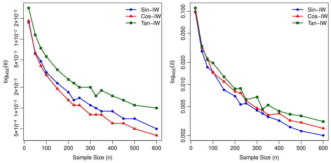
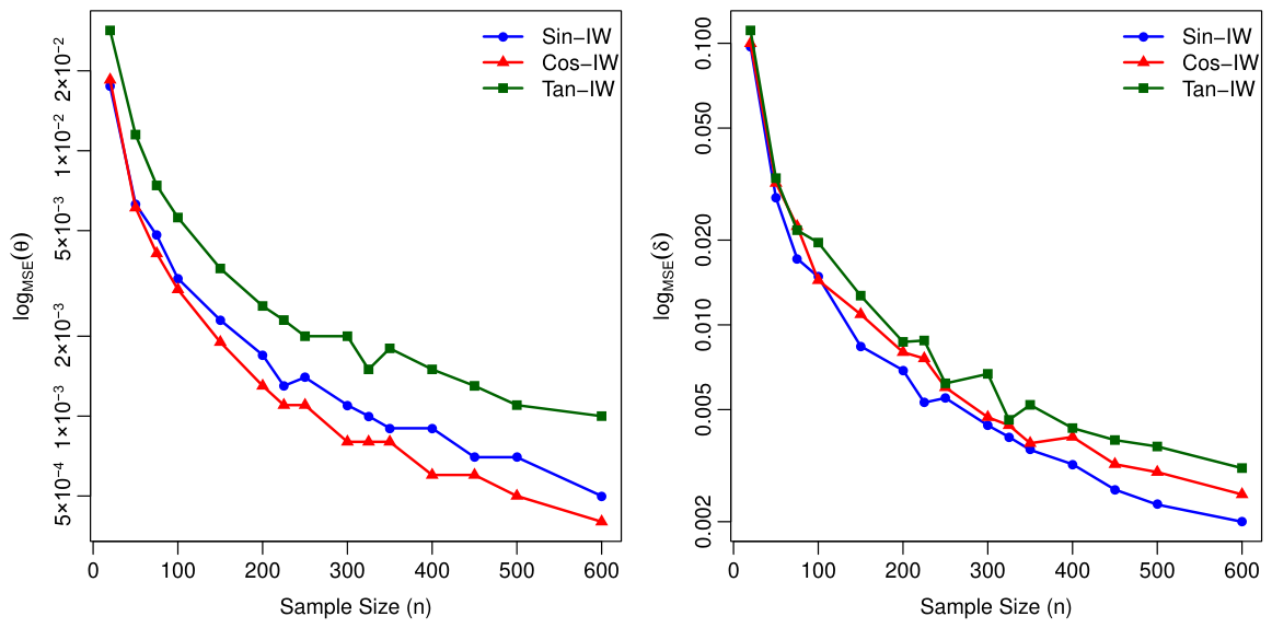
We have displayed Figure 4 and Figure 5 to show the behavior of the MSE of the MLEs for the different sample sizes. For all competing models, the MSE decreases monotonically as n increases, demonstrating the consistency of the estimators.

For the estimation of $\theta$, the Sin-IW model consistently attains the smallest MSE across all sample sizes, followed by the Cos-IW and Tan-IW models for both combinations of the parameter values. A similar pattern is observed for the estimation of $\delta$, where the Sin-IW distribution again provides lower MSE values, particularly for moderate and large n. These findings indicate that the Sin-IW distribution yields more efficient and stable parameter estimates compared with the competing models.

To ensure stable convergence and avoid local maxima, several starting values were used. The simulation results demonstrate good numerical behavior, with small biases and decreasing MSEs as the sample size increases, confirming the stability and reliability of the estimation procedure. No boundary or convergence issues were encountered.

5. Model Analysis Under Classical Approach

This section presents the performance of Sin-IW, Cos-IW, and Tan-IW models across six real datasets with varying distributional properties, as displayed in

Table 1. Real datasets taken under study.

Data	Nature of Data	Field of Data
First	Right-skewed	Annual flood discharge [31]
Second	Symmetric	Carbon fibers strength [32]
Third	Right-skewed	Time to failure (in hours) of non-repairable item [33]
Fourth	Moderately skewed to left	Stress strength (20 mm) [39]
Fifth	Extreme natured (right-skewed)	Failure time of secondary reactor pump [40]
Sixth	Left-skewed	Failure time of turbocharger engine [34]

. The results are analyzed using various goodness-of-fit measures, including $LL$ (−2 log-likelihood), $Ak$ (Akaike Information Criterion), $Ha$ (Hannan–Quinn Information Criterion), $Ko$ (Kolmogorov–Smirnov test), $Cr$ (Cramér–von Mises test), and $An$ (Anderson–Darling test). The numerical findings provide insights into the model’s suitability for specific data types.

We performed a comprehensive assessment of model adequacy and goodness-of-fit using six datasets with varying distributional characteristics. The model parameters for all datasets were estimated using R software [38], with the results presented in

Table 2. Estimated parameters via MLE for all datasets.

Dataset	Model	MLE ($\mathit{\theta }$)	SE ($\mathit{\theta }$)	MLE ($\mathit{\delta }$)	SE ($\mathit{\delta }$)
Dataset 1	Sin-IW$(\theta ,\delta )$	250.4181	5.8009	1.4413	0.0302
	Cos-IW$(\theta ,\delta )$	382.0023	5.8943	1.8150	0.0391
	Tan-IW$(\theta ,\delta )$	330.1769	60.2361	1.6534	0.0000
Dataset 2	Sin-IW$(\theta ,\delta )$	82.1700	11.7775	3.9904	0.0939
	Cos-IW$(\theta ,\delta )$	96.1949	8.3862	5.1201	0.1544
	Tan-IW$(\theta ,\delta )$	198.0995	10.9831	5.4992	0.1359
Dataset 3	Sin-IW$(\theta ,\delta )$	13.9463	6.7834	0.6321	0.1296
	Cos-IW$(\theta ,\delta )$	8.7345	5.0002	0.7766	0.1744
	Tan-IW$(\theta ,\delta )$	20.5398	8.6401	0.9365	0.1505
Dataset 4	Sin-IW$(\theta ,\delta )$	19.2054	4.0897	3.2869	0.2580
	Cos-IW$(\theta ,\delta )$	11.6772	2.6083	3.8756	0.3035
	Tan-IW$(\theta ,\delta )$	26.4137	12.2067	4.5819	0.5750
Dataset 5	Sin-IW$(\theta ,\delta )$	0.8415	0.1575	0.5733	0.0868
	Cos-IW$(\theta ,\delta )$	0.2668	0.0740	0.7382	0.1186
	Tan-IW$(\theta ,\delta )$	0.3230	0.1014	0.8753	0.1318
Dataset 6	Sin-IW$(\theta ,\delta )$	17.5600	4.1722	1.5932	0.1478
	Cos-IW$(\theta ,\delta )$	9.7835	2.9386	1.8285	0.2005
	Tan-IW$(\theta ,\delta )$	21.5128	4.4422	2.1832	0.1688

. We have also plotted the profile log-likelihood plots for all models using all six datasets. It was observed that the MLEs were consistent and unique throughout all datasets. We have presented these figures in the Supplementary Document (see Figures S1–S18). Additionally, the numerical results of the fit statistics are detailed in

Table 3. Various statistics of model selection and goodness-of-fit for all datasets.

Dataset	Models	$\mathit{LL}$	$\mathit{Ak}$	$\mathit{Ha}$	$\mathit{Ko}$	${\mathit{P}}_{\left(\mathit{Ko}\right)}$	$\mathit{Cr}$	${\mathit{P}}_{\left(\mathit{Cr}\right)}$	$\mathit{An}$	${\mathit{P}}_{\left(\mathit{An}\right)}$
Dataset 1	Sin-IW	433.4989	437.4989	438.9131	0.0774	0.9359	0.0498	0.8799	0.3721	0.8753
	Cos-IW	434.4624	438.4624	439.8766	0.1022	0.6972	0.0870	0.6543	0.6226	0.6260
	Tan-IW	445.1538	449.1538	450.5680	0.1567	0.1894	0.2963	0.1384	1.9811	0.0943
Dataset 2	Sin-IW	114.0071	118.0071	119.6930	0.0918	0.6631	0.0730	0.7352	0.3958	0.8524
	Cos-IW	118.3911	122.3911	124.0769	0.1003	0.5508	0.1039	0.5676	0.6472	0.6038
	Tan-IW	117.9621	121.9621	123.6479	0.0834	0.7736	0.0908	0.6337	0.6946	0.5628
Dataset 3	Sin-IW	114.6208	118.6208	117.9570	0.1732	0.8771	0.0581	0.8375	0.3814	0.8642
	Cos-IW	116.1048	120.1048	119.4410	0.1950	0.7741	0.0806	0.6992	0.5000	0.7426
	Tan-IW	115.5502	119.5502	118.8863	0.2070	0.7121	0.0875	0.6599	0.5035	0.7391
Dataset 4	Sin-IW	124.1826	128.1826	130.0208	0.1118	0.3138	0.3106	0.1261	2.0372	0.0878
	Cos-IW	138.7360	142.7360	144.5743	0.1505	0.0701	0.4919	0.0415	3.2354	0.0209
	Tan-IW	137.7420	141.7420	143.5802	0.1509	0.0686	0.5830	0.0244	3.5394	0.0148
Dataset 5	Sin-IW	64.5246	68.5246	69.0958	0.0796	0.9960	0.0249	0.9913	0.2429	0.9739
	Cos-IW	66.1875	70.1875	70.7587	0.1010	0.9545	0.0425	0.9239	0.3565	0.8894
	Tan-IW	65.3202	69.3202	69.8914	0.1012	0.9537	0.0410	0.9316	0.3307	0.9126
Dataset 6	Sin-IW	193.6850	197.6850	198.9063	0.2016	0.0774	0.4803	0.0442	2.8049	0.0347
	Cos-IW	203.6574	207.6574	208.8787	0.2508	0.0130	0.6078	0.0209	3.4885	0.0157
	Tan-IW	202.9251	206.9251	208.1463	0.2277	0.0316	0.6968	0.0125	3.7790	0.0113

. The summarized findings across all datasets are discussed below.

• Dataset 1 (Right-skewed Data): The first dataset, representing annual flood discharge, exhibits a right-skewed distribution. The Sin-IW model achieved the lowest $Ak$ (437.4989) and $Ha$ (438.9131), indicating superior fitting capacity. Furthermore, the minimum value of the $Ko$ statistic (0.0774) and the maximum value of its p-value (0.9359), as compared to Cos-IW and Tan-IW, confirm the model’s appropriate fit. Comparatively, Cos-IW and Tan-IW models showed higher $Ak$ values of 438.4624 and 456.1090, respectively, making Sin-IW the most appropriate model for this dataset.
• Dataset 2 (Symmetric Data): For the symmetric carbon fiber strength dataset, the Sin-IW model again showed better performance, with the smallest $Ak$ (118.0071) and $Ha$ (119.6930). The minimum $Ko$ statistic (0.0918) and maximum p-value (0.6631) supported its superior fit. Cos-IW and Tan-IW models had slightly higher $Ak$ values of 122.3911 and 121.9621, respectively. This indicates Sin-IW’s robustness in capturing symmetric data characteristics.
• Dataset 3 (Right-skewed Data): The third dataset, representing the time to failure of non-repairable items, exhibited a right-skewed distribution. Although all models performed comparably, the Sin-IW model achieved the lowest $Ak$ (118.6208) and $Ha$ (117.9570). The minimum $Ko$ statistic (0.1732) with a maximum p-value (0.8771) suggests a reasonable fit. Thus, Sin-IW is the recommended model for right-skewed data.
• Dataset 4 (Moderately Left-skewed Data): The moderately left-skewed dataset representing stress strength showed that Sin-IW outperformed Cos-IW and Tan-IW models, with the lowest $Ak$ (128.1826) and $Ha$ (130.0208). The minimum $Ko$ statistic (0.1118) and maximum p-value (0.3138) further validated the model’s effectiveness. Cos-IW and Tan-IW had higher $Ak$ values of 142.7360 and 141.7420, respectively. Sin-IW is the best choice for moderately left-skewed data.
• Dataset 5 (Extremely Right-skewed Data): For the extremely right-skewed dataset on the failure time of secondary reactor pumps, Sin-IW achieved the lowest $Ak$ (68.5246) and $Ha$ (69.0958), with a minimum $Ko$ statistic of 0.0796 and a highly significant p-value (0.9960). However, Cos-IW and Tan-IW exhibited relatively poor performance, with higher $Ak$ values of 70.1875 and 69.3202, respectively. These findings highlight Sin-IW’s superior fitting capacity for data with extreme right skewness.
• Dataset 6 (Left-skewed Data): The left-skewed dataset of turbocharger engine failure times showed that Sin-IW performed the best. It achieved the lowest $Ak$ (112.0453) and $Ha$ (113.0019) values. The minimum $Ko$ statistic (0.0831) with a maximum p-value (0.8542) confirmed an adequate fit. Cos-IW and Tan-IW exhibited relatively poor performance, with higher $Ak$ values of 117.1398 and 118.9825, respectively.

Summary of findings: The Sin-IW model consistently demonstrated superior performance across all datasets, achieving the lowest $Ak$ and $Ha$ values along with favorable goodness-of-fit measures. Further, the Sin function is monotonic near zero and introduces a smooth and gradual transformation of the baseline distribution, which results in improved tail flexibility. When combined with the heavy-tailed IW baseline, this transformation produces models that better capture skewness and tail behavior, leading to improved empirical fit compared with the Cos-G and Tan-G families.

Table 4. Best-performing models for each dataset.

Dataset	Nature of Data	Best Model	$\mathit{Ak}$	$\mathit{Ko}$ (p-Value)
1	Right-skewed	Sin-IW	437.4989	0.0774 (0.9359)
2	Symmetric	Sin-IW	118.0071	0.0918 (0.6631)
3	Right-skewed	Sin-IW	118.6208	0.1732 (0.8771)
4	Moderately left-skewed	Sin-IW	128.1826	0.1118 (0.3138)
5	Extremely right-skewed	Sin-IW	68.5246	0.0796 (0.9960)
6	Left-skewed	Sin-IW	197.685	0.2016 (0.0774)

provides an overview of the best-performing models for each dataset. Additionally, the findings indicate that the trigonometric family of distributions, particularly the Sin-G models, is especially well-suited for modeling right-skewed data compared to other data types. Based on this study, practitioners seeking to apply trigonometric statistical models are recommended to prioritize the Sin-G family and its specific models, such as Sin-IW, for effective and robust data modeling.

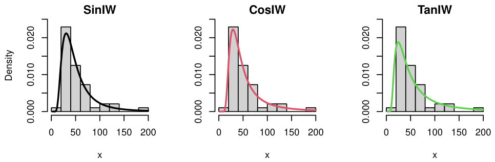
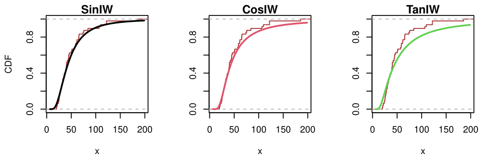
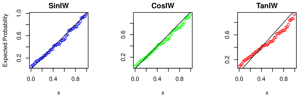
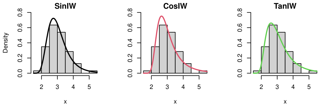
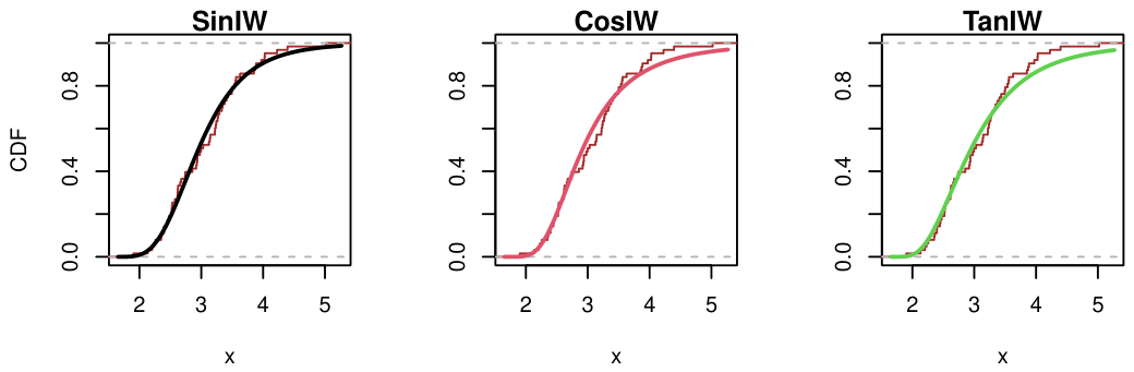
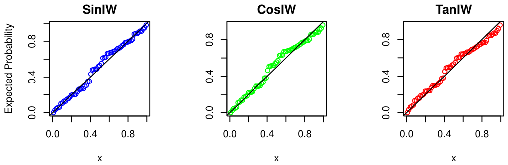
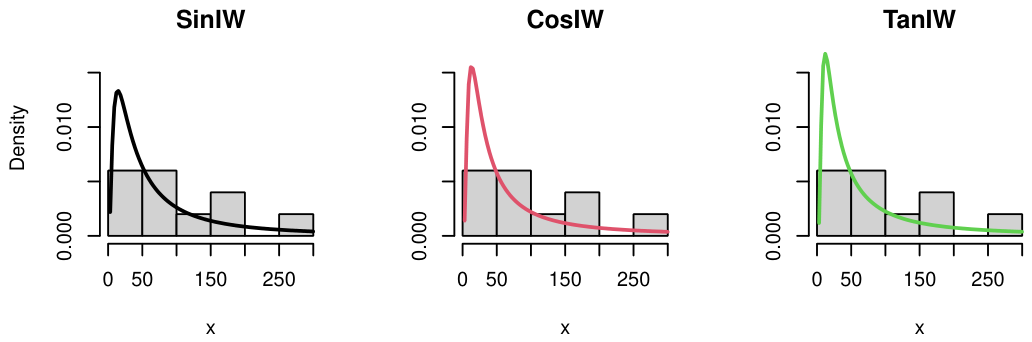
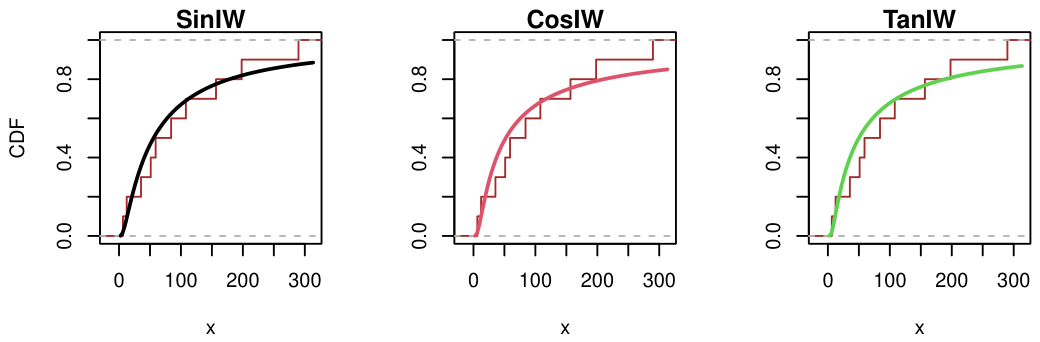
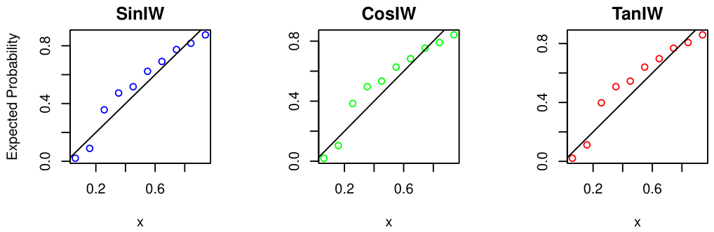
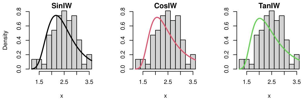
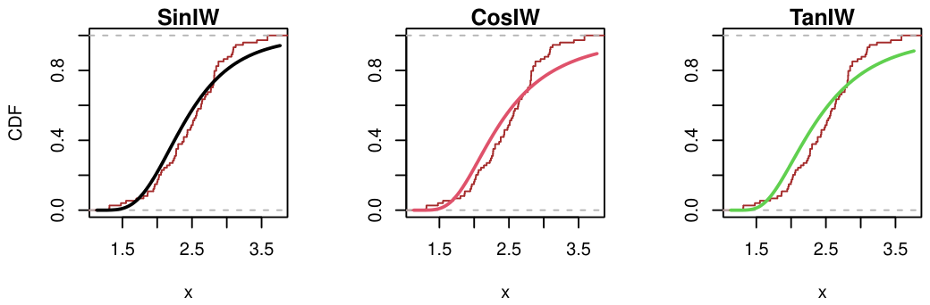
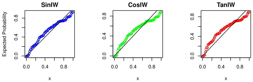
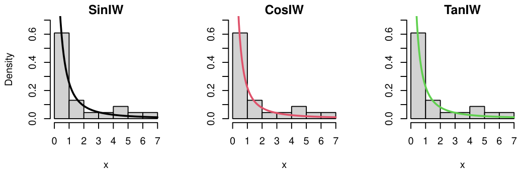
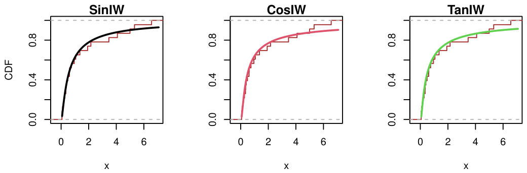
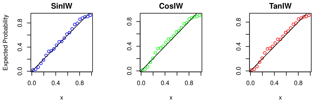
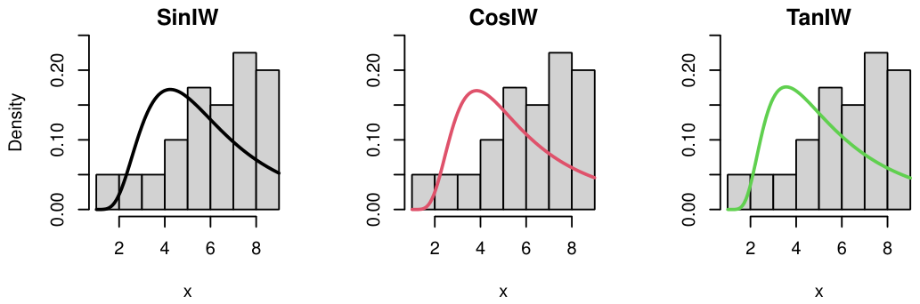
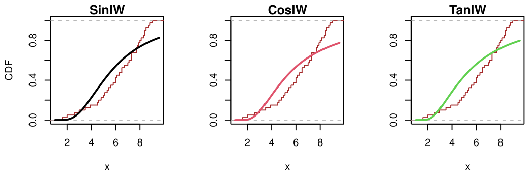
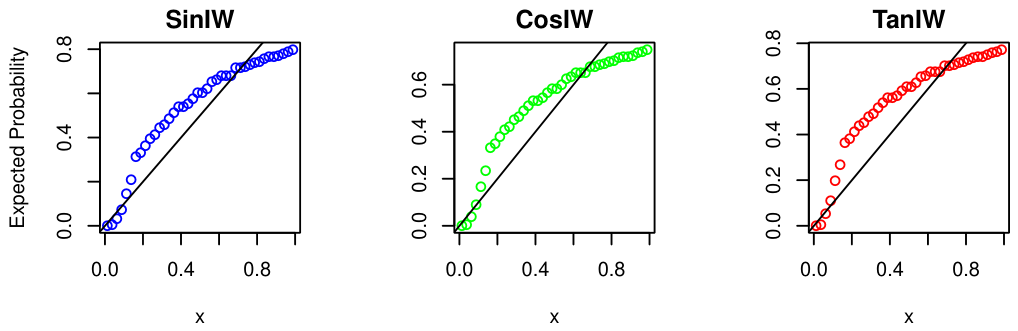
We have visually assessed the performance of the models using the fitted PDFs, CDFs, and P–P plots. Figure 6, Figure 7 and Figure 8 present the PDF, CDF, and P–P plots of the Sin-IW, Cos-IW, and Tan-IW distributions, respectively, for the first dataset. Figure 9, Figure 10 and Figure 11 present the PDF, CDF, and P–P plots of the Sin-IW, Cos-IW, and Tan-IW distributions, respectively, for the second dataset. Figure 12, Figure 13 and Figure 14 present the PDF, CDF, and P–P plots of the Sin-IW, Cos-IW, and Tan-IW distributions, respectively, for the third dataset. Figure 15, Figure 16 and Figure 17 present the PDF, CDF, and P–P plots of the Sin-IW, Cos-IW, and Tan-IW distributions, respectively, for the fourth dataset. Figure 18, Figure 19 and Figure 20 present the PDF, CDF, and P–P plots of the Sin-IW, Cos-IW, and Tan-IW distributions, respectively, for the fifth dataset. Figure 21, Figure 22 and Figure 23 present the PDF, CDF, and P–P plots of the Sin-IW, Cos-IW, and Tan-IW distributions, respectively, for the sixth dataset.

Among the three models, the Sin-IW model demonstrated superior performance, particularly in fitting right-skewed data. However, all three models exhibited relatively poor fits for left-skewed data compared to right-skewed data. To know more about the comparative performance of the Sin-G, Cos-G, and Tan-G families based on the Weibull distribution as the baseline model, readers are referred to the Supplementary Materials.

The shape of the Sin-IW density function is mainly controlled by parameters $\theta$ and $\delta$. The parameter $\theta$ acts as a scale parameter; increasing $\theta$ leads to a faster decay of $Z=\exp (-\theta x^{-\delta })$, which concentrates more probability mass near smaller values of x and results in a lighter right tail. On the other hand, the parameter $\delta$ governs the shape and tail behavior of the distribution. Larger values of $\delta$ produce sharper peaks and heavier tails, while smaller values yield smoother and more gradually decaying density curves. Through the Sin-based transformation, these parameters jointly provide sufficient flexibility for modeling datasets with varying degrees of skewness and tail heaviness.

Performance on left-skewed data: The comparatively weaker performance of the proposed models for left-skewed datasets can be attributed to the inherent right-skewed and heavy-tailed nature of the IW baseline distribution. Although trigonometric generators enhance flexibility, their transformations operate on a baseline that is not naturally suited for capturing pronounced left-skewness. As a result, model adaptability is reduced in such cases compared to right-skewed or symmetric data structures. This observation suggests that the use of alternative baseline distributions or reflection-based transformations may offer improved performance for strongly left-skewed data, which remains a potential avenue for future investigation.

6. Model Analysis Under Bayesian Approach

In this section, we analyze and compare our three proposed well-known trigonometric families of distributions using the Bayesian approach. For brevity and focus, we apply this approach to two specific datasets: a right-skewed dataset (first dataset) and a left-skewed dataset (sixth dataset).

6.1. Bayesian Inference for the Sin-IW Distribution

The Bayesian approach to parameter estimation is preferred when practitioners seek to integrate prior beliefs into the model. It integrates prior beliefs with observed data to form a posterior distribution, offering a probabilistic update of the parameters. In this analysis, we used the datasets I and VI described in Section 5. In the Bayesian approach, parameters are treated as random and assigned a prior distribution representing initial beliefs. As new data are collected, the prior is updated with the likelihood, producing a posterior distribution that reflects the revised belief about the parameter [41]. Consider the observed data represented by $\underline{x}=(x_1,\dots ,x_n)$ and the parameter of interest as $\psi$. The relationship between the observed data and the prior distribution $h\left(\psi \right)$ is captured by the likelihood function $L(\underline{x}\mid \psi )$, which is defined as

$$\begin{array}{cc}\hfill L\left(\underline{x}\right|\theta ,\delta )& ={\left({\displaystyle \frac{\pi }{2}}\theta \delta \right)}^n{\displaystyle \prod _{i=1}^n}{x}_i^{-(\delta +1)}{Z}_i\cos \left({\displaystyle \frac{\pi }{2}}{Z}_i\right).\hfill \end{array}$$

The joint distribution of the data and parameter vector can be expressed as the product of the prior distribution and the likelihood function, as follows:

$$\begin{array}{cc}\hfill f(& \underline{x};\theta ,\delta )=\left[{\left({\displaystyle \frac{\pi }{2}}\theta \delta \right)}^n{\displaystyle \prod _{i=1}^n}{x}_i^{-(\delta +1)}\cos \left({\displaystyle \frac{\pi }{2}}{Z}_i\right)Z_i\right]\left[{\displaystyle \frac{a^b}{\mathsf{\Gamma }\left(b\right)}}{e}^{-a\theta }{\theta }^{b-1}\right]\left[{\displaystyle \frac{c^d}{\mathsf{\Gamma }\left(d\right)}}{e}^{-c\delta }{\delta }^{d-1}\right].\hfill \end{array}$$

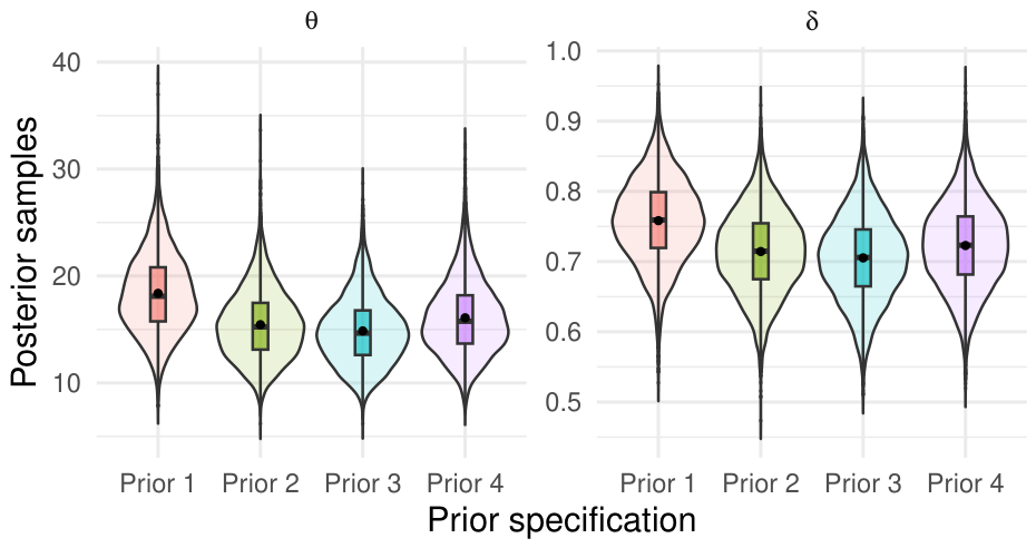
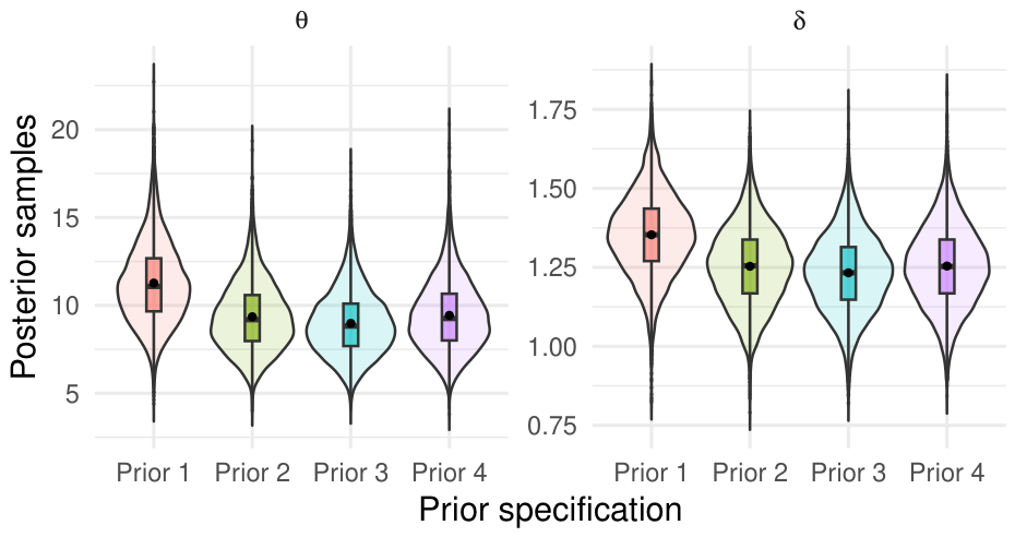
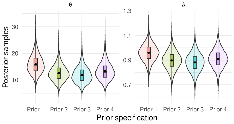
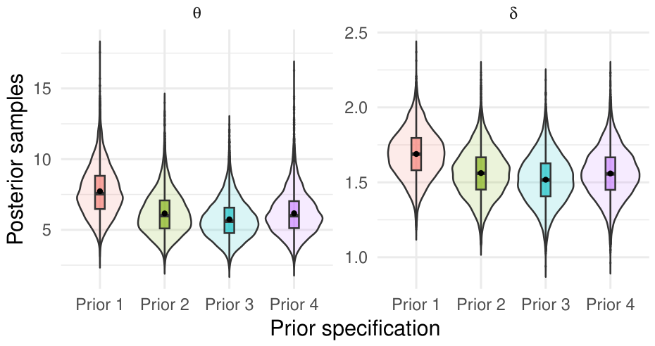
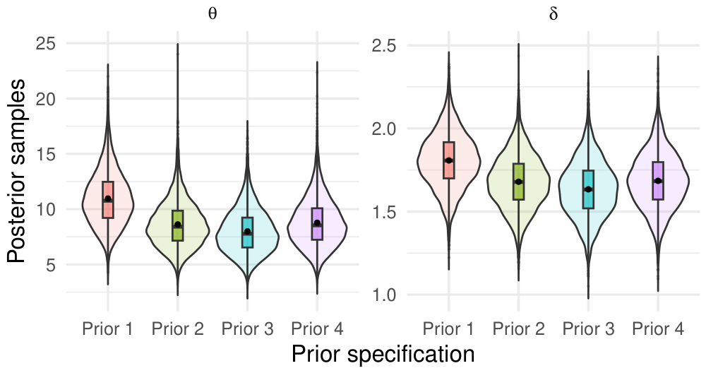
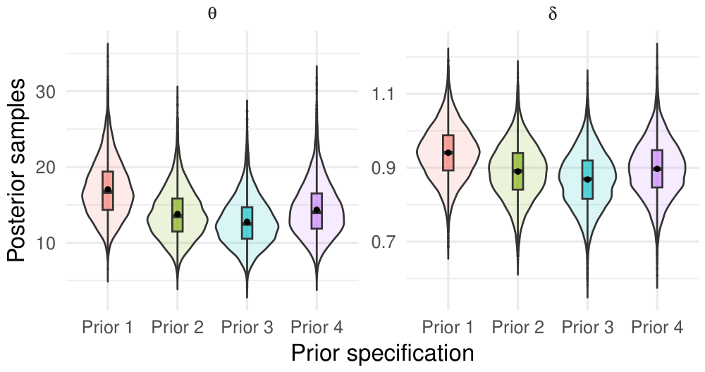
We used weakly informative Gamma priors, $\mathrm{Gamma}(a,b)$ and $\mathrm{Gamma}(c,d)$, for the parameters $\theta$ and $\delta$ of the Sin-IW distribution, with respective parameters $(a,b)$ and $(c,d)$. Since all parameters of the Sin-IW distribution lie on the positive real line, the Gamma distribution, defined over the positive real line and flexible to capture a wide range of distributional behaviors, is a great choice for the prior. Gamma priors have also been employed in similar studies [5,42]. Thus, Gamma priors are used in this study. Hyperpriors are determined based on their predictive performance using the Leave-One-Out Information Criterion (LOOIC) and the Widely Applicable Information Criterion (WAIC). Among the considered alternatives, the combination of $Gamma(5,1)$ and $Gamma(2,1)$ yields the least LOOIC and WAIC values for both datasets and is therefore selected. The LOOIC and WAIC values for all models under different prior specifications, for both datasets, are provided in

Table 5. Comparison of models based on priors, LOOIC, and WAIC.

Dataset	Model	Priors	LOOIC	WAIC
Annual flood discharge data	Sin-IW	$\theta \sim G(5,1)$ and $\delta \sim G(2,1)$	471.96	471.96
	Sin-IW	$\theta \sim G(1,1)$ and $\delta \sim G(1,1)$	476.97	476.97
	Sin-IW	$\theta \sim G(0.1,1)$ and $\delta \sim G(0.1,1)$	478.87	478.87
	Sin-IW	$\theta \sim G(0.5,0.9)$ and $\delta \sim G(0.5,0.9)$	475.93	475.93
	Cos-IW	$\theta \sim G(5,1)$ and $\delta \sim G(2,1)$	474.39	474.39
	Cos-IW	$\theta \sim G(1,1)$ and $\delta \sim G(1,1)$	480.07	480.07
	Cos-IW	$\theta \sim G(0.1,1)$ and $\delta \sim G(0.1,1)$	481.53	481.53
	Cos-IW	$\theta \sim G(0.5,0.9)$ and $\delta \sim G(0.5,0.9)$	478.78	478.78
	Tan-IW	$\theta \sim G(5,1)$ and $\delta \sim G(2,1)$	493.48	493.48
	Tan-IW	$\theta \sim G(1,1)$ and $\delta \sim G(1,1)$	499.22	499.22
	Tan-IW	$\theta \sim G(0.1,1)$ and $\delta \sim G(0.1,1)$	500.88	500.88
	Tan-IW	$\theta \sim G(0.5,0.9)$ and $\delta \sim G(0.5,0.9)$	498.09	498.09
Failure time of engine	Sin-IW	$\theta \sim G(5,1)$ and $\delta \sim G(2,1)$	199.65	199.65
	Sin-IW	$\theta \sim G(1,1)$ and $\delta \sim G(1,1)$	202.15	202.12
	Sin-IW	$\theta \sim G(0.1,1)$ and $\delta \sim G(0.1,1)$	203.04	203.03
	Sin-IW	$\theta \sim G(0.5,0.9)$ and $\delta \sim G(0.5,0.9)$	202.02	202.01
	Cos-IW	$\theta \sim G(5,1)$ and $\delta \sim G(2,1)$	207.90	207.82
	Cos-IW	$\theta \sim G(1,1)$ and $\delta \sim G(1,1)$	209.74	209.71
	Cos-IW	$\theta \sim G(0.1,1)$ and $\delta \sim G(0.1,1)$	210.33	210.33
	Cos-IW	$\theta \sim G(0.5,0.9)$ and $\delta \sim G(0.5,0.9)$	209.72	209.72
	Tan-IW	$\theta \sim G(5,1)$ and $\delta \sim G(2,1)$	209.59	209.57
	Tan-IW	$\theta \sim G(1,1)$ and $\delta \sim G(1,1)$	212.99	212.98
	Tan-IW	$\theta \sim G(0.1,1)$ and $\delta \sim G(0.1,1)$	214.39	214.38
	Tan-IW	$\theta \sim G(0.5,0.9)$ and $\delta \sim G(0.5,0.9)$	212.87	212.85

. Furthermore, prior sensitivity of the posterior distributions is examined using violin plots of posterior samples for each parameter across both datasets. The violin plots are presented in Figure 24 and Figure 25. The violin plots show that $\theta$ exhibits mild sensitivity to prior hyperparameters and $\delta$ shows minor sensitivity in terms of location; however, neither parameter is sensitive to the distributional form.

The posterior distribution of the parameters is obtained by updating the prior distribution with the likelihood function based on the sample $\underline{x}=(x_1,\dots ,x_n)$. The resulting posterior distribution is given by

$$\begin{array}{cc}\hfill f(\theta ,\delta \mid \underline{x})& \propto {\left({\displaystyle \frac{\pi }{2}}\theta \delta \right)}^n{\theta }^{b-1}{\delta }^{d-1}\exp (-a\theta -c\delta ){\displaystyle \prod _{i=1}^n}{x}_i^{-(\delta +1)}{Z}_i\cos \left({\displaystyle \frac{\pi }{2}}{Z}_i\right).\hfill \end{array}$$

Although full conditional distributions (FCDs) are not required for parameter estimation when using the Hamiltonian Monte Carlo (HMC) algorithm, Gibbs sampling techniques do require them. Therefore, we have simplified the joint posterior distribution to derive the following FCDs for each of the parameters.

The FCD of $\theta$ is expressed as

$$\begin{array}{cc}\hfill f_1\left(\theta \right|\underline{x},\delta )& \propto e^{-a\theta }{\theta }^{b+n-1}\left\{{\displaystyle \prod _{i=1}^n}{Z}_i\cos \left({\displaystyle \frac{\pi }{2}}{Z}_i\right)\right\}.\hfill \end{array}$$

The FCD of $\delta$ is expressed as

$$\begin{array}{cc}\hfill f_2\left(\delta \right|\underline{x},\theta )& \propto e^{-c\delta }{\delta }^{d+n-1}\left\{{\displaystyle \prod _{i=1}^n}{x}_i^{-(\delta +1)}{Z}_i\cos \left({\displaystyle \frac{\pi }{2}}{Z}_i\right)\right\}.\hfill \end{array}$$

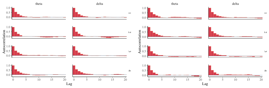
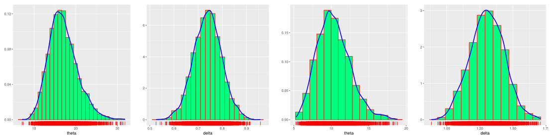
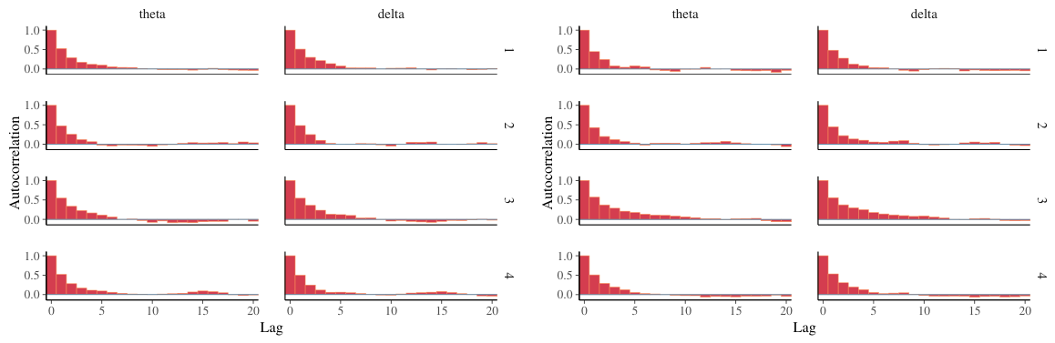
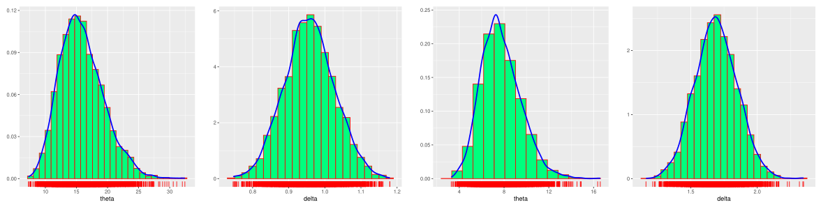
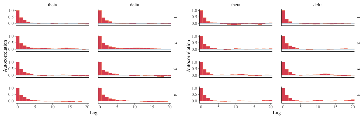
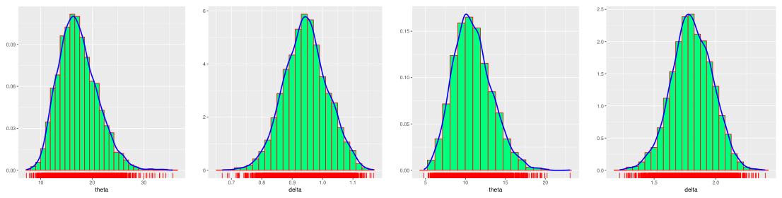
We conducted a Bayesian analysis using Stan [43] in R with 2000 iterations across four chains each. The priors for the model parameters were chosen as $Gamma(5,1)$ and $Gamma(2,1)$. The convergence diagnostics, including trace plots and autocorrelation plots, confirmed the reliability of the posterior samples (see Figure 26 and Figure 27). The trace plots appeared smooth, and the autocorrelation plots showed a decreasing trend toward zero as the lag increased. This indicates that the Markov chains mixed well and converged to the posterior distributions. The histograms of the Sin-IW model parameters obtained from the posterior samples are shown in Figure 28 for both datasets. These histograms indicate that the posterior distributions of the estimated parameters exhibit a normal shape. In addition, the effective sample sizes exceed 10% of the total samples, and the $\widehat{R}$ values are close to 1 (see

Table 6. Summary statistics of the posterior samples for Sin-IW.

Dataset	Parameter	mean	se_mean	sd	CI	HPD	n_eff	$\widehat{\mathit{R}}$
Dataset 1	$\theta$	16.9358	0.1024	3.4462	(11.0783, 24.6141)	(10.7718, 24.0447)	1133	1.0012
	$\delta$	0.7389	0.0017	0.0578	(0.6237, 0.8570)	(0.6353, 0.8654)	1116	1.0015
	log−posterior	−246.8630	0.0280	0.9975	(−249.5110, −245.8800)	(−248.9220, −245.8560)	1270	1.0026
Dataset 6	$\theta$	10.3258	0.0703	2.2020	(6.6210, 15.1199)	(5.9515, 14.3936)	982	1.0047
	$\delta$	1.3052	0.0041	0.1287	(1.0543, 1.5611)	(1.0418, 1.5365)	973	1.0040
	log−posterior	−103.9000	0.0300	1.0306	(−106.6940, −102.8840)	(−106.1100, −102.8550)	1177	1.0022

), indicating that the sampling process has stabilized and is reliably capturing the posterior distributions. Table 6 presents the summary statistics of the posterior parameter distributions for Datasets 1 and 6.

6.2. Bayesian Inference for the Cos-IW Distribution

Consider the observed data represented by $\underline{x}=(x_1,\dots ,x_n)$ and the parameter of interest as $\psi$. The connection between the observed data and the prior distribution $h\left(\psi \right)$ is captured by the likelihood function $L(\underline{x}\mid \psi )$ and expressed as follows:

$$\begin{array}{cc}\hfill L\left(\underline{x}\right|\theta ,\delta )& ={\left({\displaystyle \frac{\pi }{2}}\theta \delta \right)}^n{\displaystyle \prod _{i=1}^n}{x}_i^{-(\delta +1)}{Z}_i\sin \left({\displaystyle \frac{\pi }{2}}{Z}_i\right).\hfill \end{array}$$

Following the same guidelines as for the Sin-IW distribution, Gamma priors are also used for Cos-IW. The prior hyperparameters were selected based on the smallest LOOIC and WAIC values (see Table 5), followed by a sensitivity analysis to assess the influence of prior specifications on the posterior estimates. Violin plots of the posterior distributions under different prior hyperparameter settings are presented in Figure 29 and Figure 30. The plots indicate that $\theta$ exhibits mild sensitivity to the choice of prior hyperparameters, whereas $\delta$ appears to be less sensitive. In terms of distributional form, neither parameter is sensitive to the choice of prior hyperparameters.

The joint distribution of the data and parameter vector is obtained by multiplying the prior distribution by the likelihood function, as given below:

$$\begin{array}{cc}\hfill f(\theta ,\delta |\underline{x})& \propto \left\{{\left({\displaystyle \frac{\pi }{2}}\theta \delta \right)}^n{\displaystyle \prod _{i=1}^n}{x}_i^{-(\delta +1)}{Z}_i\sin ({\displaystyle \frac{\pi }{2}}{Z}_i)\right\}\times \left\{e^{-a\theta }{\theta }^{b-1}{e}^{-c\delta }{\delta }^{d-1}\right\}.\hfill \end{array}$$

The FCD of $\theta$ is expressed as

$$\begin{array}{cc}\hfill f_1\left(\theta \right|\underline{x},\delta )& \propto e^{-a\theta }{\theta }^{b+n-1}\left\{{\displaystyle \prod _{i=1}^n}{Z}_i\sin ({\displaystyle \frac{\pi }{2}}{Z}_i)\right\}.\hfill \end{array}$$

The FCD of $\delta$ is expressed as

$$\begin{array}{cc}\hfill f_2\left(\delta \right|\underline{x},\theta )& \propto e^{-c\delta }{\delta }^{d+n-1}\left\{{\displaystyle \prod _{i=1}^n}{x}_i^{-(\delta +1)}{Z}_i\sin ({\displaystyle \frac{\pi }{2}}{Z}_i)\right\}.\hfill \end{array}$$

The convergence diagnostics for the Cos-IW distribution parameters of interest across both datasets—including trace plots and autocorrelation plots (see Figure 31 and Figure 32)—provide strong evidence for the reliability and stability of the posterior samples. The trace plots appeared smooth, and the autocorrelation plots showed a decreasing trend toward zero as the lag increased. This indicates that the Markov chains mixed well and converged to the posterior distributions. The histograms of the Cos-IW model parameters obtained from the posterior samples are shown in Figure 33 for both datasets. These histograms indicate that the posterior distributions of the estimated parameters exhibit a normal shape. In addition, the effective sample sizes exceed 10% of the total samples, and the $\widehat{R}$ values are close to 1 (see

Table 7. Summary statistics of the posterior samples for Cos-IW.

Dataset	Parameter	mean	se_mean	sd	CI	HPD	n_eff	$\widehat{\mathit{R}}$
Dataset 1	$\theta$	15.8679	0.1032	3.5377	(9.9339, 23.6359)	(9.4843, 23.0270)	1174	1.0021
	$\delta$	0.9574	0.0020	0.0694	(0.8260, 1.0967)	(0.8276, 1.0972)	1166	1.0030
	log−posterior	−240.3780	0.0278	1.0026	(−243.1330, −239.3870)	(−242.3660, −239.3630)	1302	1.0015
Dataset 6	$\theta$	7.7348	0.0530	1.7650	(4.7611, 11.5353)	(4.7005, 11.3713)	1108	1.0024
	$\delta$	1.6907	0.0049	0.1594	(1.3815, 2.0092)	(1.3697, 1.9927)	1045	1.0039
	log−posterior	−101.3030	0.0278	1.0072	(−104.0280, −100.3250)	(−103.3950, −100.3020)	1314	1.0026

), indicating that the sampling process has stabilized and is reliably capturing the posterior distributions. Table 7 presents the summary statistics of the posterior parameter distributions for Datasets 1 and 6.

6.3. Bayesian Inference for the Tan-IW Distribution

Consider the observed data represented by $\underline{x}=(x_1,\dots ,x_n)$ and the parameter of interest as $\psi$. The connection between the observed data and the prior distribution $h\left(\psi \right)$ is captured by the likelihood function $L(\underline{x}\mid \psi )$ and expressed as follows:

$$\begin{array}{cc}\hfill L\left(\underline{x}\right|\theta ,\delta )& ={\left({\displaystyle \frac{\pi }{4}}\theta \delta \right)}^n{\displaystyle \prod _{i=1}^n}{x}_i^{-(\delta +1)}{Z}_i{\sec }^2\left({\displaystyle \frac{\pi }{4}}{Z}_i\right).\hfill \end{array}$$

By following the same reasoning as for the Sin-IW and Cos-IW distributions, Gamma priors and their hyperparameters are also applied to the Tan-IW distribution. Sensitivity analysis of the prior hyperparameters for the Tan-IW distribution was conducted using violin plots of the posterior distributions of the parameter estimates. The violin plots are presented in Figure 34 and Figure 35. The results indicate that $\theta$ exhibits mild sensitivity to the choice of prior hyperparameters, whereas $\delta$ appears to be relatively robust and less sensitive to these specifications. In terms of distributional form, neither parameter is sensitive to the choice of prior hyperparameters.

The joint posterior distribution of the parameters is obtained by updating the prior distribution with the likelihood function. The resulting posterior distribution is given by

$$\begin{array}{cc}\hfill f(& \theta ,\delta |\underline{x})\propto \left\{{\left({\displaystyle \frac{\pi }{4}}\theta \delta \right)}^n{\displaystyle \prod _{i=1}^n}{x}_i^{-(\delta +1)}{Z}_i{\sec }^2\left({\displaystyle \frac{\pi }{4}}{Z}_i\right)\right\}\left\{{\displaystyle \frac{a^b}{\mathsf{\Gamma }\left(b\right)}}{e}^{-a\theta }{\theta }^{b-1}\right\}\left\{{\displaystyle \frac{c^d}{\mathsf{\Gamma }\left(d\right)}}{e}^{-c\delta }{\delta }^{d-1}\right\}.\hfill \end{array}$$

The FCD of the parameter $\theta$ is given by

$$\begin{array}{cc}\hfill f_1\left(\theta \right|\underline{x},\delta )& \propto e^{-a\theta }{\theta }^{b+n-1}\left\{{\displaystyle \prod _{i=1}^n}{Z}_i{\sec }^2\left({\displaystyle \frac{\pi }{4}}{Z}_i\right)\right\}.\hfill \end{array}$$

The FCD of the parameter $\delta$ is given by

$$\begin{array}{c}\hfill f_2\left(\delta \right|\underline{x},\theta )\propto e^{-c\delta }{\delta }^{d+n-1}\left\{{\displaystyle \prod _{i=1}^n}{x}_i^{-(\delta +1)}{Z}_i{\sec }^2\left({\displaystyle \frac{\pi }{4}}{Z}_i\right)\right\}.\end{array}$$

The convergence diagnostics for the Tan-IW distribution parameters of interest across both datasets—including trace plots and autocorrelation plots (see Figure 36 and Figure 37)—provide strong evidence for the reliability and stability of the posterior samples. The trace plots exhibit stable, well-mixed chains, while the autocorrelation plots display a clear decay toward zero with increasing lag, suggesting good mixing and convergence of the Markov chains to the target posterior distributions. Additionally, the histograms of the Tan-IW model parameters derived from the posterior samples (Figure 38) demonstrate approximately normal-shaped distributions for both datasets. The effective sample sizes exceed 10% of the total iterations, and the corresponding $\widehat{R}$ values are close to 1 (see

Table 8. Summary statistics of the posterior samples for Tan-IW.

Dataset	Parameter	mean	se_mean	sd	CI	HPD	n_eff	$\widehat{\mathit{R}}$
Dataset 1	$\theta$	17.2479	0.1050	3.7633	(11.0089, 25.6027)	(10.2585, 24.3675)	1284	1.0010
	$\delta$	0.9443	0.0021	0.0721	(0.8035, 1.0872)	(0.8068, 1.0891)	1151	1.0003
	log−posterior	−250.7620	0.0257	0.9957	(−253.3610, −249.7780)	(−252.6950, −249.7560)	1497	1.0017
Dataset 6	$\theta$	10.9088	0.0611	2.4296	(6.6984, 16.2451)	(6.3962, 15.7238)	1583	1.0037
	$\delta$	1.8066	0.0041	0.1656	(1.4699, 2.1195)	(1.4742, 2.1241)	1595	1.0045
	log−posterior	−104.1440	0.0244	0.9660	(−106.7210, −103.1830)	(−106.0850, −103.1590)	1571	0.9996

), further confirming that the sampling process has stabilized and is effectively capturing the posterior distributions. Table 8 summarizes the posterior parameter estimates for Dataset 1 and 6.

6.4. Model Comparison for the First Data

We evaluated three models, Sin-IW, Cos-IW, and Tan-IW, using the Widely Applicable Information Criterion (WAIC), computed from a $4000\times 48$ log-likelihood matrix. The WAIC results for each model are summarized in

Table 9. WAIC metrics for the three models and model comparison of the first data.

Metric	Sin-IW	cos-IW	Tan-IW
$elp{d}_{waic}$ (SE)	−237.20 (4.9)	−237.30 (4.9)	−246.80 (4.7)
$p_{waic}$ (SE)	0.40 (0.0)	0.30 (0.0)	0.30 (0.0)
$waic$ (SE)	474.40 (9.9)	474.60 (9.8)	493.50 (9.4)
Model Comparison
$elp{d}_{diff}$	0.00	−0.10	−9.60
${\mathrm{SE}}_{diff}$	0.00	0.10	0.40

.

Model Sin-IW demonstrated an expected log predictive density ($elp{d}_{waic}$) of $-237.2$ with a standard error (SE) of 4.9, a WAIC value of 474.4 (SE = 9.9), and an effective number of parameters ($p_{waic}$) of 0.4 (SE = 0.0). Similarly, Cos-IW yielded an $elp{d}_{waic}$ of $-237.3$ (SE = 4.9), a WAIC of 474.6 (SE = 9.8), and $p_{waic}=0.3$ (SE = 0.0). Model Tan-IW had a slightly worse performance, with an $elp{d}_{waic}$ of $-246.8$ (SE = 4.7), a WAIC of 493.5 (SE = 9.4), and $p_{waic}=0.3$ (SE = 0.0). To compare the relative performance of these models, we computed the differences in $elp{d}_{waic}$ ($elp{d}_{diff}$) between models. As shown in Table 9, Sin-IW served as the baseline model ($elp{d}_{diff}=0.0$, $SE=0.0$), with Cos-IW showing a negligible difference ($elp{d}_{diff}=-0.1$, $SE=0.1$). However, Tan-IW exhibited a significant decline in predictive accuracy compared to Sin-IW, with $elp{d}_{diff}=-9.6$ (SE = 0.4). While the Sin-IW model attained the smallest WAIC, the difference in predictive performance between the Sin-IW and Cos-IW distributions was small compared to its uncertainty, because $|{elpd}_{diff}|<2{\mathrm{SE}}_{diff}$. Thus, these two distributions have comparable predictive performance. In contrast, the Tan-IW distribution shows poorer predictive accuracy because $|{elpd}_{diff}|>2{\mathrm{SE}}_{diff}$.

These results suggest that Sin-IW and Cos-IW perform similarly, whereas Tan-IW shows reduced predictive capability, making it less suitable for this first data.

6.5. Model Comparison for the Sixth Data

The WAIC was also computed to evaluate the predictive performance of three models for the sixth dataset (left-skewed): Sin-IW, Cos-IW, and Tan-IW. The computations were based on a $4000\times 40$ log-likelihood matrix for each model.

Table 10. WAIC metrics for the three models and model comparison for the sixth data.

Metric	Sin-IW	Cos-IW	Tan-IW
$elp{d}_{waic}$	−100.30 (2.7)	−104.00 (3.8)	−104.90 (2.7)
$p_{waic}$	1.10 (0.5)	1.70 (1.0)	0.80 (0.4)
$waic$	200.60 (5.4)	207.90 (7.6)	209.70 (5.4)
Model Comparison
$elp{d}_{diff}$	0.00	−3.60	−4.50
${\mathrm{SE}}_{diff}$	0.00	1.50	1.00

summarizes the results, including $elp{d}_{waic}$, $p_{waic}$, and the WAIC values, along with their associated SE.

• The Sin-IW model had an $elp{d}_{waic}$ of $-100.3$ (SE = 2.7), a $p_{waic}$ of 1.1 (SE = 0.5), and a WAIC of 200.6 (SE = 5.4).
• The Cos-IW model showed slightly worse performance, with an $elp{d}_{waic}$ of $-104.0$ (SE = 3.8), a $p_{waic}$ of 1.7 (SE = 1.0), and a WAIC of 207.9 (SE = 7.6).
• Similarly, the Tan-IW model yielded an $elp{d}_{waic}$ of $-104.9$ (SE = 2.7), a $p_{waic}$ of 0.8 (SE = 0.4), and a WAIC of 209.7 (SE = 5.4).

To further compare the models, $elp{d}_{diff}$ and ${\mathrm{SE}}_{diff}$ were calculated (see Table 10). The Sin-IW model had an ($elp{d}_{diff}=0.0$, ${\mathrm{SE}}_{diff}=0.0$). The Cos-IW model had an $elp{d}_{diff}$ of $-3.6$ (SE = 1.5), indicating a slightly lower predictive accuracy compared to Sin-IW. The Tan-IW model demonstrated the lowest performance, with an $elp{d}_{diff}$ of $-4.5$ (SE = 1.0).

The differences in predictive performance between the Sin-IW and Cos-IW distributions and between the Sin-IW and Tan-IW distributions exceeded twice their corresponding standard errors. Thus, Sin-IW distributions provide a better predictive performance over both the Cos-IW and Tan-IW distributions for the sixth dataset.

Based on these findings, Sin-IW can be considered the most suitable model for the left-skewed data, also.

6.6. Computational Efficiency and Time Complexity

To evaluate computational efficiency, wall-clock run-time was recorded for both classical and Bayesian estimation procedures. Classical estimation was carried out using simulation-based methods, whereas Bayesian estimation was implemented via HMC in Stan. In the classical simulation studies, the Sin-IW, Cos-IW, and Tan-IW models required approximately 1.76 min, 1.74 min, and 4.00 min, respectively, with the Tan-IW model exhibiting a higher computational cost.

Bayesian estimation showed comparatively lower run-time in the application analyses. For the first dataset, the Sin-IW, Cos-IW, and Tan-IW models required approximately 16.04 s, 9.30 s, and 12.26 s, respectively, while for the second dataset, the corresponding run-times were 7.46 s, 7.12 s, and 9.30 s.

Hence, classical simulation-based estimation was computationally more demanding, whereas the Bayesian approach implemented in Stan demonstrated efficient performance. These results indicate that Bayesian estimation remains computationally feasible for flexible IW-type base models.

7. Conclusions

This study highlights the comparative analysis of trigonometric families of distributions, sine-G, cosine-G, and tangent-G, across diverse data structures. Furthermore, it provides a systematic, application-oriented comparison of trigonometric families under a common Inverse Weibull baseline distribution. In the classical approach, the Sin-G family of distributions performed better than both the Cos-G and Tan-G families with the IW baseline across all data shapes, including right-skewed, left-skewed, and symmetric cases. In the Bayesian approach, the Sin-G family also performed best for both right- and left-skewed data compared to the other two families; however, the performance difference was more pronounced for left-skewed data than for right-skewed data. While comparing datasets, all three trigonometric families performed best for right-skewed data and showed weaker performance for left-skewed datasets; however, among the three families, the Sin-G family consistently performed best. A similar pattern of performance was also observed under the Bayesian approach. This is because the HRF plots show that all three models can generate flexible shapes, including decreasing and unimodal hazard functions. This behavior is closely related to the empirical results. Right-skewed lifetime data are commonly associated with decreasing or early-failure hazard patterns, which are well captured by the Sin-G, Cos-G, and Tan-G families with the heavy-tailed IW baseline. This flexibility may partly explain the relatively strong performance of the Sin-G family for right-skewed datasets. In contrast, symmetric and left-skewed data may be associated with hazard structures that are more challenging for the proposed framework to capture, which may partly explain the relatively weaker performance. These findings provide valuable insights for researchers and data scientists working with trigonometric models in data analysis.

It should be noted that the observed better performance of the Sin-G family in this study is conditional on the IW baseline distribution, the selected datasets, and the estimation framework employed. While the results provide strong empirical evidence within this setting, they should not be interpreted as universal dominance across all baseline distributions or data scenarios.

8. Limitations and Future Directions

8.1. Limitations

Despite the important contribution of this paper in comparing the trigonometric family of distributions across a variety of data settings, the study is not free from limitations. The following are some notable limitations of this study.

• In this study, we utilized the IW distribution as the base distribution and datasets used to compare the sine-G, cosine-G, and tangent-G families. While this choice provided meaningful insights, different base distributions could lead to varying results for similar types of data. Future studies should explore additional base distributions to assess the generalizability of our findings.
• Although the classical analysis included all six datasets, the Bayesian analysis was limited to two representative datasets (right-skewed and left-skewed) to illustrate model behavior under different distributional settings. However, future studies may extend the analysis to a broader range of distributional shapes and more complex data structures.

8.2. Future Directions

• Future work may extend the present study by considering trigonometric families generated from alternative parent distributions to examine the robustness of the proposed comparisons beyond the IW baseline. In addition, further extensions may involve broader Bayesian analyses using diverse data settings and the application of additional model comparison criteria to support model selection.
• Future studies may also benchmark the trigonometric-G families against non-trigonometric alternatives, such as the Weibull, inverse Weibull, and other generalized distributions, to gain broader insight into their comparative performance.
• Recent developments in optimization, such as Distributionally Robust Bayesian Optimization via Sinkhorn-Based Wasserstein Barycenter [44], also offer a potential avenue for extending such comparisons within modern optimization frameworks.
• Current trigonometric distributions based on the IW baseline are limited to analyzing univariate data. However, real applications may involve multivariate data, underscoring the need to extend these univariate trigonometric distributions to multivariate settings. In addition to developing multivariate models based on the IW baseline, future research may also explore other baseline distributions and generalize them to multivariate frameworks.

References

1. Tomy, L.; Dominic, L. Review on Distributions Generated Using Trigonometric Functions. Austrian J. Stat. 2024, 53, 102–119. [Google Scholar] [CrossRef] [Scilit]
2. Raab, D.H.; Green, E.H. A cosine approximation to the normal distribution. Psychometrika 1961, 26, 447–450. [Google Scholar] [CrossRef] [Scilit]
3. Wu, J.J.M. Extreme statistics from the cosine distribution. Commun. Stat.-Theory Methods 2000, 29, 1397–1403. [Google Scholar] [CrossRef] [Scilit]
4. Burrows, P.M. Extreme statistics from the Sine distribution. Am. Stat. 1986, 40, 216. [Google Scholar] [CrossRef] [Scilit]
5. Mohammad, S.; Cooray, K. Modeling actuarial data using iterated trigonometric distributions. Commun. Stat.-Theory Methods 2025, 54, 5112–5128. [Google Scholar]
6. Kumar, D.; Singh, U.; Singh, S.K. A new distribution using Sine function-its application to bladder cancer patients data. J. Stat. Appl. Probab. 2015, 4, 417–427. [Google Scholar]
7. Souza, L.; Junior, W.; De Brito, C.; Chesneau, C.; Ferreira, T.; Soares, L. On the Sin-G class of distributions: Theory, model and application. J. Math. Model. 2019, 7, 357–379. [Google Scholar] [CrossRef] [Scilit]
8. Souza, L.; Junior, W.R.O.; de Brito, C.C.R.; Ferreira, T.A.E.; Soares, L.G.M. General properties for the Cos-G class of distributions with applications. Eurasian Bull. Math. 2019, 2, 63–79. [Google Scholar]
9. Souza, L.; Júnior, W.R.O.; Brito, C.C.R.; Chesneau, C.; Fernandes, R.L.; Ferreira, T.A.E. Tan-G class of trigonometric distributions and its applications. Cubo 2021, 23, 1–20. [Google Scholar] [CrossRef] [Scilit]
10. Sapkota, L.P.; Kumar, P.; Kumar, V. A New Class of Sin-G Family of Distributions with Applications to Medical Data. Reliab. Theory Appl. 2023, 18, 734–750. [Google Scholar]
11. Kumar, P.; Sapkota, L.P.; Kumar, V. A New Class of Tan-G Family of Distributions with Properties and Applications. South East Asian J. Math. Math. Sci. 2023, 19, 393–420. [Google Scholar] [CrossRef] [Scilit]
12. Sapkota, L.P.; Kumar, P.; Kumar, V.; Tashkandy, Y.A.; Bakr, M.E.; Balogun, O.S.; Mekiso, G.T.; Gemeay, A.M. Sine π-power odd-G family of distributions with applications. Sci. Rep. 2024, 14, 19481. [Google Scholar] [CrossRef] [Scilit] [PubMed]
13. Kumar, P.; Sapkota, L.P.; Kumar, V.; Tashkandy, Y.A.; Bakr, M.E.; Balogun, O.S.; Gemeay, A.M. A new class of cosine trigonometric lifetime distribution with applications. Alex. Eng. J. 2024, 106, 664–674. [Google Scholar] [CrossRef] [Scilit]
14. Benchiha, S.; Sapkota, L.P.; Al Mutairi, A.; Kumar, V.; Khashab, R.H.; Gemeay, A.M.; Elgarhy, M.; Nassr, S.G. A new Sine family of generalized distributions: Statistical inference with applications. Math. Comput. Appl. 2023, 28, 83. [Google Scholar] [CrossRef] [Scilit]
15. Mahmood, Z.; Chesneau, C.; Tahir, M.H. A new Sine-G family of distributions: Properties and applications. Bull. Comput. Appl. Math. 2019, 7, 53–81. [Google Scholar]
16. Al-Babtain, A.A.; Elbatal, I.; Chesneau, C.; Elgarhy, M. Sine Topp-Leone-G family of distributions: Theory and applications. Open Phys. 2020, 18, 574–593. [Google Scholar] [CrossRef] [Scilit]
17. Chesneau, C.; Jamal, F. The Sine Kumaraswamy-G family of distributions. J. Math. Ext. 2020, 15, 2. [Google Scholar] [CrossRef] [Scilit]
18. Oramulu, D.O.; Alsadat, N.; Kumar, A.; Bahloul, M.M.; Obulezi, O.J. Sine generalized family of distributions: Properties, estimation, simulations and applications. Alex. Eng. J. 2024, 109, 532–552. [Google Scholar] [CrossRef] [Scilit]
19. Sakthivel, K.M.; Rajkumar, J. Transmuted Sine-G family of distributions: Theory and applications. Stat. Appl. 2021, 20, 2. [Google Scholar]
20. Jamal, F.; Chesneau, C.; Bouali, D.L.; Ul Hassan, M. Beyond the Sin-G family: The transformed Sin-G family. PLoS ONE 2021, 16, e0250790. [Google Scholar] [CrossRef] [Scilit] [PubMed]
21. Fayomi, A.; Algarni, A.; Almarashi, A.M. Sine inverse Lomax generated family of distributions with applications. Math. Probl. Eng. 2021, 2021, 1267420. [Google Scholar] [CrossRef] [Scilit]
22. Abonongo, J.; Mwaniki, I.J.; Aduda, J.A. Sine F-Loss Family of Distributions: Properties and Insurance Applications. Appl. Math. Inf. Sci. 2022, 16, 835–851. [Google Scholar] [CrossRef] [Scilit]
23. Isa, A.M.; Doguwa, S.I.; Alhaji, B.B.; Dikko, H.G. Sine Type II Topp-Leone G Family of Probability Distribution: Mathematical Properties and Application. Arid Zone J. Basic Appl. Res. 2023, 2, 124–138. [Google Scholar] [CrossRef] [Scilit]
24. Chesneau, C.; Bakouch, H.S.; Karakaya, K.; Bazyari, A. The Sine Modified Power-Generated Family of Distributions with Application to Practical Data and Ruin Probability. Lobachevskii J. Math. 2023, 44, 4643–4662. [Google Scholar] [CrossRef] [Scilit]
25. Rajkumar, J.; Sakthivel, K.M. A new method of generating Marshall–Olkin Sine–G family and its applications in survival analysis. Lobachevskii J. Math. 2022, 43, 463–472. [Google Scholar] [CrossRef] [Scilit]
26. Sapkota, L.P.; Alsahangiti, A.M.; Kumar, V.; Gemeay, A.M.; Bakr, M.E.; Balogun, O.S.; Muse, A.H. Arc-tangent exponential distribution with applications to weather and chemical data under classical and Bayesian approach. IEEE Access 2023, 11, 115462–115476. [Google Scholar] [CrossRef] [Scilit]
27. Odhah, O.H.; Alshanbari, H.M.; Ahmad, Z.; Rao, G.S. A weighted cosine-G family of distributions: Properties and illustration using time-to-event data. Axioms 2023, 12, 849. [Google Scholar] [CrossRef] [Scilit]
28. Al-Mofleh, H. On generating a new family of distributions using the tangent function. Pak. J. Stat. Oper. Res. 2018, 14, 471–499. [Google Scholar] [CrossRef] [Scilit]
29. Tomy, L.; G, V.; Chesneau, C. The Sine Modified Lindley Distribution. Math. Comput. Appl. 2021, 26, 81. [Google Scholar] [CrossRef] [Scilit]
30. Muhammad, M.; Alshanbari, H.M.; Alanzi, A.R.A.; Liu, L.; Sami, W.; Chesneau, C.; Jamal, F. New Generator of Probability Models: The Exponentiated Sine-G Family for Lifetime Studies. Entropy 2021, 23, 1394. [Google Scholar] [CrossRef] [Scilit] [PubMed]
31. Van Montfort, M.A.J. On testing that the distribution of extremes is of type I when type II is the alternative. J. Hydrol. 1970, 11, 421–427. [Google Scholar] [CrossRef] [Scilit]
32. Kundu, D.; Gupta, R.D. Estimation of P(Y < X) for Weibull Distributions. IEEE Trans. Reliab. 2006, 55, 270–280. [Google Scholar] [CrossRef] [Scilit]
33. Murthy, D.N.P.; Xie, M.; Jiang, R. Weibull Models; John Wiley & Sons: Hoboken, NJ, USA, 2004. [Google Scholar]
34. Xu, K.; Xie, M.; Tang, L.C.; Ho, S.L. Application of neural networks in forecasting engine systems reliability. Appl. Soft Comput. 2003, 2, 255–268. [Google Scholar] [CrossRef] [Scilit]
35. Kundu, D.; Howlader, H. Bayesian inference and prediction of the inverse Weibull distribution for Type-II censored data. Comput. Stat. Data Anal. 2010, 54, 1547–1558. [Google Scholar] [CrossRef] [Scilit]
36. Alkarni, S.; Afify, A.Z.; Elbatal, I.; Elgarhy, M. The extended inverse Weibull distribution: Properties and applications. Complexity 2020, 2020, 3297693. [Google Scholar] [CrossRef] [Scilit]
37. Henningsen, A.; Toomet, O. maxLik: A package for maximum likelihood estimation in R. Comput. Stat. 2011, 26, 443–458. [Google Scholar]
38. R Core Team. R: A Language and Environment for Statistical Computing; R Foundation for Statistical Computing: Vienna, Austria, 2024; Available online: https://www.R-project.org/ (accessed on 29 June 2026).
39. Kundu, D.; Raqab, M.Z. Estimation of R = P(Y < X) for three-parameter Weibull distribution. Stat. Probab. Lett. 2009, 79, 1839–1846. [Google Scholar] [CrossRef] [Scilit]
40. Suprawhardana, M.S.; Prayoto, S. Total time on test plot analysis for mechanical components of the RSG-GAS reactor. At. Indones. 1999, 25, 81–90. [Google Scholar]
41. Gelman, A.; Rubin, D.B. Inference from Iterative Simulation Using Multiple Sequences. Stat. Sci. 1992, 7, 457–472. [Google Scholar] [CrossRef] [Scilit]
42. Sapkota, L.P.; Kumar, P.; Kumar, V.; Bam, N. Estimation and Analysis of Trigonometric Models under Bayesian Approach. Pak. J. Stat. Oper. Res. 2024, 20, 587–613. [Google Scholar] [CrossRef] [Scilit]
43. Stan Development Team. The Stan Core Library. Version 2.31.0, 2022. Available online: http://mc-stan.org/ (accessed on 25 May 2026).
44. Seyedi, I.; Candelieri, A.; Archetti, F. Distributionally Robust Bayesian Optimization via Sinkhorn-Based Wasserstein Barycenter. Mach. Learn. Knowl. Extr. 2025, 7, 90. [Google Scholar] [CrossRef] [Scilit]
Figure 1. Illustration of various PDF and HRF curve shapes of the Sin-IW.
Data 11 00182 g001
Figure 2. Illustration of various PDF and HRF curve shapes of the Cos-IW.
Data 11 00182 g002
Figure 3. Illustration of various PDF and HRF curve shapes of the Tan-IW.
Data 11 00182 g003
Figure 4. MSE plots of Sin-IW, Cos-IW, and Tan-IW for θ = 0.5 and δ = 1.5 .
Data 11 00182 g004
Figure 5. MSE plots of Sin-IW, Cos-IW, and Tan-IW for θ = 1.5 and δ = 0.5 .
Data 11 00182 g005
Figure 6. Fitted PDF of Sin-IW, Cos-IW, and Tan-IW for the first data.
Data 11 00182 g006
Figure 7. Fitted CDF of Sin-IW, Cos-IW, and Tan-IW for the first data.
Data 11 00182 g007
Figure 8. PP plots of tin-IW, Cos-IW, and Tan-IW for the first data.
Data 11 00182 g008
Figure 9. Fitted PDF of Sin-IW, Cos-IW, and Tan-IW for the second data.
Data 11 00182 g009
Figure 10. Fitted CDF of Sin-IW, Cos-IW, and Tan-IW for the second data.
Data 11 00182 g010
Figure 11. PP plots of Sin-IW, Cos-IW, and Tan-IW for the second data.
Data 11 00182 g011
Figure 12. Fitted PDF of Sin-IW, Cos-IW, and Tan-IW for the third data.
Data 11 00182 g012
Figure 13. Fitted CDF of Sin-IW, Cos-IW, and Tan-IW for the third data.
Data 11 00182 g013
Figure 14. PP plots of Sin-IW, Cos-IW, and Tan-IW for the third data.
Data 11 00182 g014
Figure 15. Fitted PDF of Sin-IW, Cos-IW, and Tan-IW for the fourth data.
Data 11 00182 g015
Figure 16. Fitted CDF of Sin-IW, Cos-IW, and Tan-IW for the fourth data.
Data 11 00182 g016
Figure 17. PP plot of Sin-IW, Cos-IW, and Tan-IW for the fourth data.
Data 11 00182 g017
Figure 18. Fitted PDF of Sin-IW, Cos-IW, and Tan-IW for the fifth data.
Data 11 00182 g018
Figure 19. Fitted CDF of Sin-IW, Cos-IW, and Tan-IW for the fifth data.
Data 11 00182 g019
Figure 20. PP plots of Sin-IW, Cos-IW, and Tan-IW for the fifth data.
Data 11 00182 g020
Figure 21. Fitted PDF of Sin-IW, Cos-IW, and Tan-IW for the sixth data.
Data 11 00182 g021
Figure 22. Fitted CDF of Sin-IW, Cos-IW, and Tan-IW for the sixth data.
Data 11 00182 g022
Figure 23. PP plots of Sin-IW, Cos-IW, and Tan-IW for the sixth data.
Data 11 00182 g023
Figure 24. Violin plots of posterior sensitivity to prior specifications for Sin-IW (Dataset 1).
Data 11 00182 g024
Figure 25. Violin plots of posterior sensitivity to prior specifications for Sin-IW (Dataset 2).
Data 11 00182 g025
Figure 26. Trace plots for the first and sixth data of Sin-IW.
Data 11 00182 g026
Figure 27. Auto-correlation plots for the first and sixth data of Sin-IW.
Data 11 00182 g027
Figure 28. Histogram of posterior estimates of the parameters for the first and sixth data of Sin-IW.
Data 11 00182 g028
Figure 29. Violin plots of posterior sensitivity to prior specifications for Cos-IW (Dataset 1).
Data 11 00182 g029
Figure 30. Violin plots of posterior sensitivity to prior specifications for Cos-IW (Dataset 6).
Data 11 00182 g030
Figure 31. Trace plots for the first and sixth data of Cos-IW.
Data 11 00182 g031
Figure 32. Auto-correlation plots for the first and sixth data of Cos-IW.
Data 11 00182 g032
Figure 33. Histogram of posterior estimates of the parameters for the first and sixth data of Cos-IW.
Data 11 00182 g033
Figure 34. Violin plots of posterior sensitivity to prior specifications for Tan-IW (Dataset 1).
Data 11 00182 g034
Figure 35. Violin plots of posterior sensitivity to prior specifications for Tan-IW (Dataset 6).
Data 11 00182 g035
Figure 36. Trace plots for the first and sixth data of Tan-IW.
Data 11 00182 g036
Figure 37. Auto-correlation plots for the first and sixth data of Tan-IW.
Data 11 00182 g037
Figure 38. Histogram of posterior estimates of the parameters for the first and sixth data of Tan-IW.
Data 11 00182 g038