An Open Industrial Energy Dataset with Asset-Level Measurements and High-Coverage 15-Minute Aggregates from a Manufacturing Facility

Abstract

Publicly available electricity datasets from operational industrial facilities remain limited due to instrumentation cost, retrofit complexity, and data governance constraints. This paper presents an openly accessible dataset of asset-level electrical energy measurements collected from a medium-scale industrial manufacturing facility over an approximately one-year observation window, with staged commissioning resulting in heterogeneous temporal coverage. The dataset includes time-series measurements from production machinery, auxiliary systems, and distribution-level assets instrumented using a heterogeneous fleet of Ethernet and RS-485 energy meters integrated via industrial gateways and programmable logic controllers. Measurements were acquired via a SCADA-based logging infrastructure and exported from an operational SQL historian. The publicly released dataset comprises fixed 15 min aggregated energy and power metrics derived from high-frequency SCADA telemetry. In its released ALL-phase representation, the dataset comprises measurements from 43 monitored assets and 1,039,873 15 min windows, corresponding to 2.96 GWh of measured electrical energy. Mean window-level data coverage is 99.99%, and 97.72% of ALL-phase windows satisfy the dataset’s reliability criterion. Interval records include energy consumption, demand, data coverage metrics, and reliability indicators. The dataset reflects real-world industrial monitoring conditions, including mixed communication pathways and irregular sampling behaviour, and is intended to support research in industrial energy analytics, data quality assessment, load profiling, and operational energy modelling.

Dataset: https://doi.org/10.5281/zenodo.19180972

Dataset License: CC BY 4.0

1. Introduction

Publicly available electricity datasets from operational industrial facilities remain scarce, particularly for small- to mid-scale manufacturing environments operating under retrofit monitoring constraints. While industry accounts for a substantial share of global final energy consumption and greenhouse gas emissions [1], empirical energy analytics research continues to rely disproportionately on simulated environments, laboratory testbeds, or building-sector datasets [2,3,4]. The limited availability of openly accessible, longitudinal industrial telemetry restricts benchmarking, reproducibility, and methodological validation in industrial energy analytics and machine learning research [3,5]. Industrial monitoring environments differ significantly from residential and commercial smart-meter contexts. Manufacturing facilities typically operate heterogeneous fleets of legacy and modern equipment integrated across multiple communication standards, control systems, and vendor-specific architectures [6,7]. Telemetry streams are frequently irregular in cadence and subject to communication jitter, partial outages, and configuration drift over time. Longitudinal operation often reveals integration-induced instabilities and instrumentation inconsistencies that are not observable in short-duration experimental setups [7]. These characteristics complicate data engineering and analysis, but they also represent the operational reality within which industrial energy optimisation must occur. Improving industrial energy efficiency remains a central research and policy priority. Despite the availability of economically viable efficiency measures, a persistent ‘energy efficiency gap’ is widely documented, often attributed to insufficient transparency, inadequate performance indicators, and limited integration of energy metrics into production decision-making systems [8]. Meaningful optimisation requires machine- and asset-level visibility rather than coarse plant-wide aggregation, particularly to identify idle loads, auxiliary consumption, and state-dependent inefficiencies [1,2]. However, such analysis depends on reliable, high-resolution telemetry coupled with explicit and reproducible data quality characterisation. Recent open dataset initiatives in the built environment have demonstrated the value of large-scale, well-documented meter datasets for benchmarking and comparative analytics [3,9]. Similarly, high-frequency household energy datasets have shown that publishing raw measurements alongside contextual metadata and known limitations can materially accelerate methodological development [5]. Yet equivalent open resources representing live industrial production settings remain comparatively rare. Where datasets are available, they are often proprietary, short-term, or curated to remove operational imperfections, limiting their value for stress testing and longitudinal analysis [4,6].

This paper presents an openly accessible industrial energy monitoring dataset comprising asset-level electrical measurements collected from a medium-scale manufacturing facility over an extended observation period. The dataset captures heterogeneous electrical loads across the generation–distribution–consumption hierarchy, including hydraulic presses, mixers, compressors, air handling units, heat pumps, utilities, and distribution boards. Measurements were acquired via a SCADA-mediated logging infrastructure integrating Ethernet-connected and legacy RS-485 energy meters through industrial gateways and programmable logic controllers (PLCs). Raw observations were archived at their native SCADA cadence, preserving real-world acquisition behaviour, including timing jitter, communication-induced latency variation, and intermittent coverage. Rather than presenting a curated or idealised dataset, the release explicitly documents instrumentation constraints, configuration faults, commissioning offsets, and coverage variability. Data quality is characterised using transparent, task-independent data quality indicators, including completeness and temporal reliability metrics, enabling users to apply context-dependent filtering policies without obscuring original measurements [10]. A structured Bronze–Silver–Gold processing architecture is provided, preserving raw exports while publishing a derived 15 min fact table constructed through deterministic forward-hold integration and explicit coverage reporting. By exposing the structural characteristics of operational industrial telemetry (i.e., heterogeneity, irregular sampling, staggered commissioning, and documented instrumentation faults), this dataset provides a realistic benchmark resource for research in industrial energy analytics, load profiling, anomaly detection, forecasting, monitoring system validation, and robustness analysis under imperfect conditions. The release is intended not as a prescriptive optimisation framework, but as a transparent reference dataset supporting reproducible, longitudinal investigation of industrial energy behaviour in live production environments. In addition to serving as a data resource, the dataset enables systematic evaluation of analytical methods under partial observability, irregular sampling, and explicitly characterised data quality constraints. The principal contributions of this data descriptor are as follows: (i) the release of an industrial electricity dataset spanning an approximately one-year observation window, with asset-level monitoring introduced progressively across that window covering 43 asset-level and distribution-level metering points at 15 min resolution; (ii) publication of explicit completeness and reliability indicators at the interval level; (iii) documentation of a reproducible Bronze–Silver–Gold processing architecture for transforming irregular SCADA telemetry into fixed-interval aggregates; and (iv) quantitative validation of the monitoring hierarchy using containment and correlation analysis.

2. Data Description

2.1. Study Context and Facility Overview

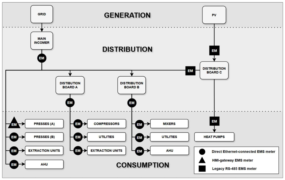
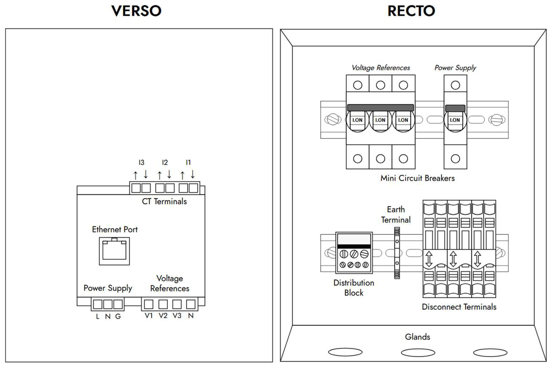
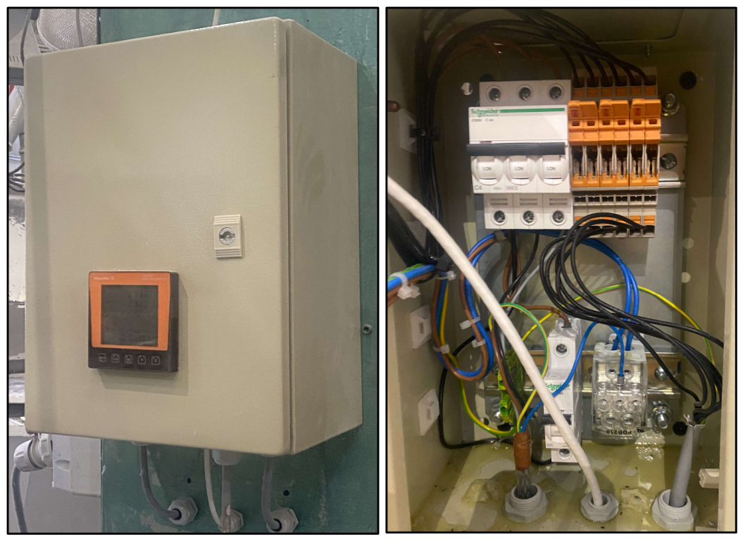
The dataset was acquired from a medium-scale manufacturing facility in Ireland employing approximately 150 personnel and operating under continuous production conditions. Data acquisition was performed under live operational constraints, with no experimental load shaping or controlled scheduling introduced. Over the four years preceding the study period, the site exhibited an annual electricity demand of approximately 1.6–1.8 GWh, placing it at the lower end of the European small-to-mid-scale manufacturing range (typically 1–10 GWh yr⁻¹) [11,12]. Facilities of this scale are increasingly targeted for retrofit energy monitoring and efficiency interventions [2,8], yet remain underrepresented in publicly available high-resolution industrial datasets. Electrical supply is provided through a dual-source configuration comprising a grid connection and on-site photovoltaic (PV) generation. Grid power feeds a central main incomer, from which electricity is distributed across downstream distribution boards serving both production and auxiliary loads. The monitored infrastructure spans the full generation–distribution–consumption chain, including distribution-level metering and asset-level sub-metering. Figure 1 illustrates the electrical topology represented within the energy monitoring system (EMS), including grid import, PV generation, distribution boundaries, and downstream asset groupings. The dataset includes a diverse set of electrically intensive assets representative of typical industrial loads, including hydraulic presses, air handling units (AHUs), compressors, heat pumps, mixers, and ancillary utilities. These assets exhibit predominantly motor-driven, inductive load profiles with variable duty cycles, intermittent operation, and phase-level variability. Such behaviours are characteristic of manufacturing environments and present non-trivial challenges for retrofit energy monitoring [1,2,6]. To ensure consistency and installation safety, asset-level monitoring was deployed using standardised EMS cabinets, a schematic of which is shown in Figure 2. Each cabinet incorporates current transformer (CT) disconnect terminals, voltage reference miniature circuit breakers (MCBs), neutral and protective earth distribution bars, and front-mounted true-RMS energy meters. This modular design enables repeatable installation across heterogeneous assets and reduces the likelihood of wiring and CT polarity errors. Figure 3 presents a physical realisation of the cabinet design, including a deployed unit (left) and its internal wiring layout (right). This hierarchical and modular instrumentation approach supports both asset-level analysis and reconciliation of energy flows across distribution boundaries, forming the basis for the dataset structure and validation procedures described in later sections.

2.2. Instrumentation and Meter Deployment

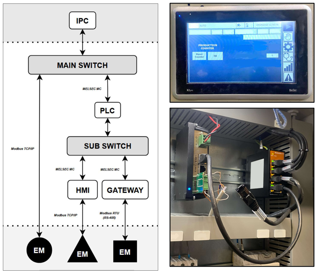
Electrical energy monitoring within the facility was implemented through a staged retrofit programme, resulting in a heterogeneous but systematically documented metering deployment. A combination of modern Ethernet-enabled energy meters and legacy RS-485 devices was employed, reflecting practical constraints commonly encountered in operational industrial environments. This mixed communication topology is illustrated in Figure 4 (left), which shows both direct Modbus TCP/IP connections and indirect PLC- and gateway-mediated data pathways to the SCADA Industrial PC (IPC). The primary instrumentation comprised Weidmüller EM220 series three-phase energy meters [13], permanently installed at both distribution-level and asset-level locations. These meters provide true-RMS measurements of phase currents, voltages, active power, apparent power, and power factor, and support sub-second internal measurement updates. In addition to these devices, four legacy Rayleigh energy meters [14,15] were retained and integrated into the monitoring network; while functionally compatible with the broader system, these legacy devices communicate exclusively via Modbus RTU [16] over RS-485 and therefore required intermediary communication hardware. Where Ethernet connectivity was locally available, energy meters were connected directly to the site’s industrial SCADA network using Modbus TCP/IP. In cases where native Ethernet connectivity was unavailable, either due to RS-485-only communication interfaces or limited physical network ports, meters were routed through IIoT-enabled HMI devices or intermediary gateways. Representative implementations are shown in Figure 4, using Beijer’s X2 Pro 10 HMI [17] (above right) and Box2 Pro gateway [18] (below right). In these configurations, meter values were polled via Modbus RTU or Modbus TCP and subsequently transferred into the SCADA environment through PLCs using the MELSEC MC [19] communication protocol.

Although functionally unified at the SCADA level, these differing communication routes introduce structural variation in data transfer latency, buffering behaviour, and timing regularity. Meter placement followed a hierarchical strategy aligned with the facility’s electrical topology. Distribution-level meters were installed at the main incomer and at selected downstream distribution boards to capture aggregated flows, including grid import and photovoltaic generation. Asset-level meters were installed on electrically intensive loads, including presses, compressors, AHUs, mixers, heat pumps, and auxiliary systems. This configuration enables both asset-specific analysis and reconciliation against upstream measurements. All meters were installed using consistent physical wiring practices, including standardised current transformer placement, voltage referencing, and protective isolation. While minor differences exist between device generations and communication pathways, the electrical instrumentation itself is homogeneous in terms of measurement intent and coverage of electrical variables.

2.3. Communication Architecture and Data Acquisition Pathways

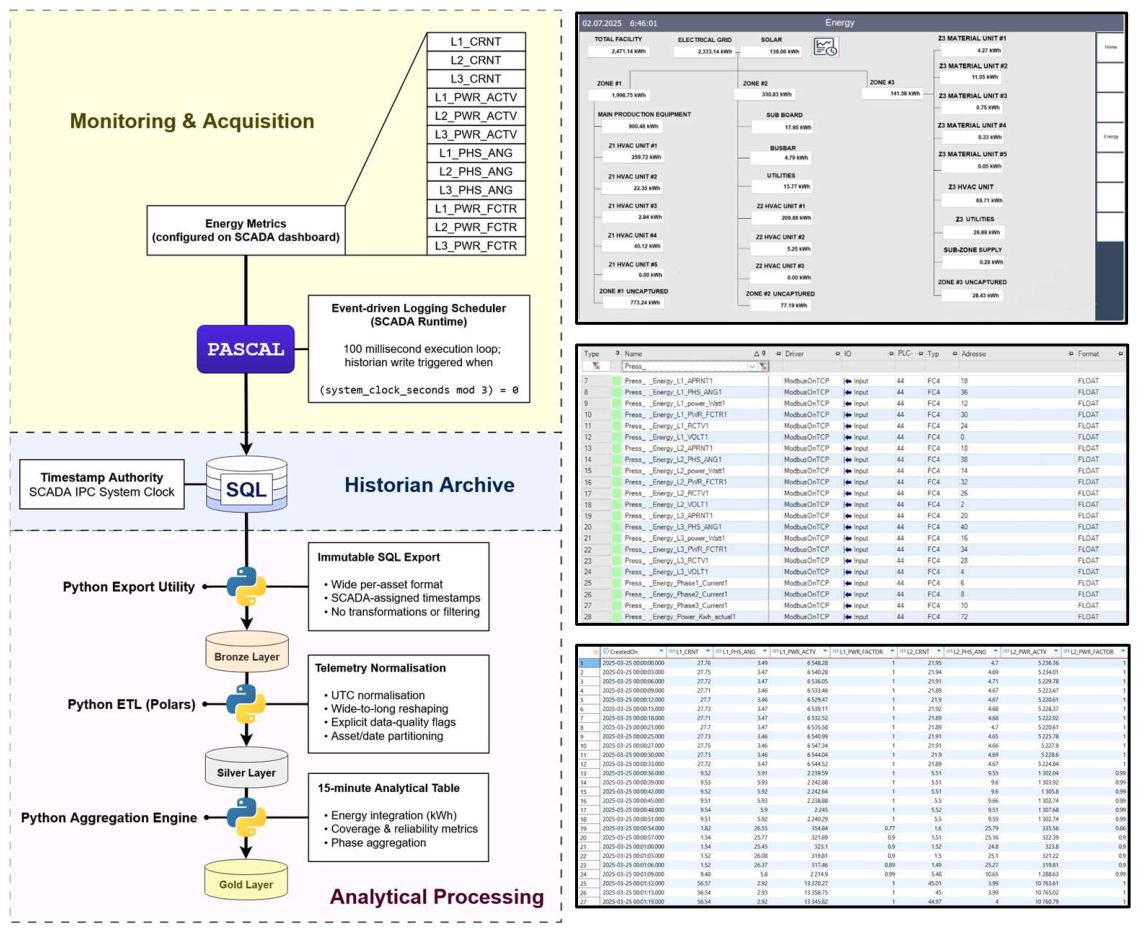
Although the deployed energy meters support native internal measurement updates at approximately 1 s resolution, all measurements used in this study were recorded centrally by the facility’s SCADA system. The complete end-to-end data acquisition and processing pipeline is summarised in Figure 5 (left), with representative SCADA dashboard views (above right), tag configuration interfaces (middle right), and raw SQL historian exports (below right).

The effective temporal resolution of the dataset is therefore determined by the SCADA-side logging architecture rather than by the intrinsic capabilities of the metering hardware. Data acquisition was performed by an IPC running the site’s SCADA software, PROCON-WEB SCADA [20], which acted as the sole logging authority for all connected energy meters. The IPC periodically polled each meter, either directly via Modbus TCP/IP or indirectly via gateway–PLC pathways, and wrote the retrieved values into an SQL-based historian database. Energy meters themselves did not persist historical records; all long-term storage was managed centrally. The SCADA logging routine operated on a global time-based scheduler derived from the IPC system clock. Timestamping occurred at the point of successful value acquisition within the SCADA runtime; no device-side timestamps were retained or reconciled, with all temporal alignment reflecting IPC clock synchronisation. Under nominal conditions, logging cycles were initiated at fixed modulo intervals of the wall-clock second, producing a nominal acquisition cadence of approximately 3 s under stable operating conditions. This scheduler governed the initiation of data requests rather than their completion, meaning that each logging cycle comprised multiple sequential steps:

• Initiation of a scheduled polling cycle by the IPC;
• Retrieval of measurement values directly from meter registers via Modbus TCP/IP, or indirectly from PLC-registers;
• Buffering and processing of retrieved values within the SCADA runtime;
• Insertion of timestamped records into the SQL historian.

Because acquisition timing was governed by the IPC scheduler and not by the meters, the effective inter-arrival time of recorded samples reflects the cumulative behaviour of the entire communication and logging chain. Variations in network latency, PLC scan cycles, gateway buffering, and database write operations may therefore introduce small deviations from the nominal logging interval, even under otherwise stable operating conditions. The architecture employed a unified logging routine for all assets, irrespective of the communication pathway. As a result, all measurements, whether sourced from directly connected Ethernet meters or from RS-485 devices routed through gateways, were timestamped using the IPC system clock and stored within a common database schema. This design ensures temporal consistency at the database level while simultaneously exposing any pathway-dependent timing effects at the level of recorded inter-arrival intervals. The SQL historian served as the authoritative source for all subsequent data processing. Periodic exports were performed to generate Parquet files, which formed the raw input to the analytical pipeline described in Section 2.4. No resampling, interpolation, or gap filling was applied during export; values were written exactly as recorded by the SCADA system, preserving both nominal cadence and any deviations arising from the acquisition process. This centralised logging architecture reflects common practice in retrofit industrial monitoring deployments, where constraints on network infrastructure, legacy equipment, and system integration necessitate IPC-mediated data capture. The implications of this design for data completeness, timing regularity, and reliability are explored quantitatively in later sections of the paper.

2.4. Temporal Scope and Logging Cadence

The dataset spans an approximately twelve-month observation period, capturing routine production, maintenance, and idle operating conditions under live industrial constraints. This duration was chosen to capture seasonal variation, workload heterogeneity, and longer-term operational patterns. However, individual assets exhibit variable temporal coverage within this window due to the staged deployment of metering infrastructure. Although the deployed energy meters internally update electrical quantities at a nominal 1 s cadence, measurements are not logged at the device level. Instead, all values are recorded centrally by the site’s SCADA IPC, which determines the effective logging interval. During the study period, the SCADA system was configured to initiate acquisition cycles on a nominal 3 s schedule. Because timestamps are assigned at the point of SCADA acquisition rather than at the meter, the effective inter-arrival time of recorded samples reflects both the scheduler configuration and the cumulative effects of communication latency, PLC scan cycles, gateway buffering, and database write operations. Consequently, the raw dataset exhibits small but measurable timing variability around the nominal logging interval. No attempt is made at this stage to regularise or resample the time series; measurements are preserved exactly as recorded by the SCADA system. All timestamps are normalised to Coordinated Universal Time (UTC) during ingestion to ensure consistency across daylight-saving transitions and to support long-horizon temporal analysis.

2.5. Raw Data Characteristics and Partitioning

For scalability and traceability, raw records are partitioned by asset identifier and UTC calendar day. This partitioning strategy supports incremental ingestion, deterministic rebuilds, and selective reprocessing of affected time ranges without requiring global dataset rewrites. It also enables efficient querying and alignment with downstream analytical workflows operating on fixed temporal windows.

2.6. Dataset Structure and File Organisation

The dataset follows a layered medallion-style processing architecture consisting of Bronze (raw exports), Silver (normalised telemetry), and Gold (fixed-interval aggregates) layers.

2.6.1. Bronze Layer (Internal Raw Exports)

The Bronze layer comprises direct SQL historian exports written to Parquet format, with one file per metered asset. These files preserve the wide-format structure generated by the SCADA system and retain all register-level measurements at their native acquisition cadence. No transformations, interpolation, or filtering were applied at this stage. Bronze files are treated as immutable archival artefacts and serve as the reproducible source for downstream processing. They are not included in the publicly released dataset.

2.6.2. Silver Layer (Internal Normalised Telemetry)

The Silver layer normalises Bronze exports into a long-format telemetry structure, producing one record per ‘AssetId’, ‘Phase’, and ‘CreatedOnUtc’. Each record includes active power (kW), apparent power (kVA), power factor, inter-arrival time, and explicit row-level data quality indicators (e.g., gap detection, missing values, physically implausible readings), along with a composite reliability flag (‘IsReliableRow’). Silver data are stored in partitioned Parquet format by asset identifier and UTC date to support incremental reprocessing and deterministic regeneration. Like the Bronze layer, Silver data are retained internally and are not publicly released, as they preserve the native high-resolution acquisition behaviour of the monitoring system.

2.6.3. Gold Layer (Publicly Released Dataset)

The publicly released dataset consists exclusively of the Gold layer: fixed 15 min interval energy and power aggregates derived from the Silver telemetry, with active power treated as magnitude for most assets, except where signed power is retained for upstream supply measurements. Silver records are interpreted using a forward-hold assumption, whereby each observation represents a piecewise-constant power segment spanning the interval until the next valid observation. These segments are intersected with fixed 15 min windows using interval-weighted integration. The schema of each daily partitioned Gold-layer file, including field names, data types, and descriptions, is summarised in

Table 1. Schema of the published 15 min Gold-layer aggregation table.

Column Name	Datatype	Description
AssetId	VARCHAR	Anonymised asset identifier
Phase	VARCHAR	Electrical phase (L1, L2, L3, ALL)
window_start_utc	TIMESTAMP	Start of 15 min aggregation window (UTC)
DateKeyUtc	INTEGER	UTC date key (YYYYMMDD)
TimeKeyUtc	INTEGER	UTC time key (HHMMSS)
WindowStartLocal	TIMESTAMP	Window start in local timezone
HourLocal	INTEGER	Local hour of day
DateLocal	DATE	Local calendar date
Energy_kWh_15m	DOUBLE	Energy consumed during window
Demand_kW	DOUBLE	Average demand over window
AvgPower_kW_15m	DOUBLE	Reliability-weighted mean power
Minutes	DOUBLE	Minutes of observed data in window
SecondsObserved	DOUBLE	Total seconds observed
DataCoveragePct	DOUBLE	Observed coverage (%)
SecondsReliable	DOUBLE	Seconds passing reliability criteria
ReliableCoveragePct	DOUBLE	Reliable coverage (%)
IsReliableWindow	INTEGER	Reliability flag (1 = reliable)

. For each ‘AssetId’, ‘Phase’, and ‘window_start_utc’, the following metrics are computed:

• Energy_kWh_15m;
• AvgPower_kW_15m;
• Demand_kW;
• SecondsObserved;
• SecondsReliable;
• DataCoveragePct;
• ReliableCoveragePct;
• IsReliableWindow.

Where applicable, phase-level records are additionally aggregated to a synthetic ‘ALL’ phase representing total asset-level consumption. By releasing interval-based aggregates rather than native high-frequency telemetry, the dataset preserves analytical value for load profiling, energy modelling, and benchmarking tasks, while mitigating exposure of fine-grained operational signatures such as sub-minute duty cycles.

2.6.4. File Format and Partitioning Scheme

The Gold dataset is stored in Apache Parquet format using columnar compression (e.g., Zstandard). Files are partitioned by asset identifier and UTC calendar date using a Hive-style directory structure:

‘asset_id=<AssetId>/dt_utc=<YYYY-MM-DD>/part-<YYYY-MM-DD>.parquet’

This partitioning scheme enables:

• Efficient subsetting by asset and time range;
• Scalable processing in analytical engines (e.g., Python, R, SQL-based systems);
• Deterministic regeneration of daily partitions;
• Compatibility with modern lakehouse-style workflows.

All timestamps are normalised to Coordinated Universal Time (UTC) prior to storage to ensure consistency across daylight-saving transitions and support long-horizon temporal analysis. Each partition contains a single deterministic file to ensure reproducibility and simplify downstream ingestion. The monitored assets included in the published dataset are summarised in

Table 2. Inventory of metered consumer assets and temporal coverage within the published dataset.

ID	Metered Asset	Asset Type	Start
ahu_a	AHU	hvac	1 January 2025
ahu_b	AHU	hvac	1 January 2025
ahu_c	AHU	hvac	1 January 2025
comp_a	Air Compressor	machine	22 May 2025
comp_b	Air Compressor	machine	22 May 2025
ex_a	Air Extractor	hvac	22 May 2025
ex_b	Air Extractor	hvac	1 January 2025
hp_a	Heat Pump	hvac	30 April 2025
hp_b	Heat Pump	hvac	30 April 2025
mh_a	Material Handling Line	machine	1 January 2025
mix_a	Material Mixer	machine	1 January 2025
mix_b	Material Mixer	machine	1 January 2025
mix_c	Material Mixer	machine	1 January 2025
mix_d	Material Mixer	machine	1 January 2025
p_a	Press Main	machine	21 February 2025
p_b	Press Main	machine	1 January 2025
p_c	Press Drive	machine	20 February 2025
p_d	Press Main	machine	20 February 2025
p_e	Press Main	machine	5 February 2025
p_f	Press Main	machine	1 January 2025
p_g	Press Main	machine	21 March 2025
p_h	Press Main	machine	20 February 2025
p_i	Press Main	machine	21 March 2025
p_j	Press Drive	machine	18 December 2025
p_k	Press Main and Robot	machine	1 January 2025
p_l	Press Main	machine	21 March 2025
p_m	Press Main	machine	21 March 2025
p_n	Press Main	machine	19 December 2025
ph_c	Press Heating	machine	17 August 2025
ph_j	Press Heating	machine	18 November 2025
pr_e	Press Robot	machine	19 November 2025
pr_f	Press Robot	machine	20 November 2025
pr_k	Press Robot	machine	18 November 2025

and

Table 3. Inventory of metered supply and distribution assets and temporal coverage within the published dataset.

ID	Metered Asset	Asset Type	Start
mi_a	Grid Connection	supply	22 May 2025
mi_b	PV Generation	supply	30 April 2025
sb_a	Sub-Distribution Board	distribution	30 April 2025
sb_b	Sub-Distribution Board	distribution	22 May 2025
sb_c	Sub-Distribution Board	distribution	23 May 2025
u_a	Utilities	utility	22 May 2025
u_b	Utilities	utility	22 May 2025
u_c	Utilities	utility	22 May 2025
u_d	Utilities	utility	1 January 2025
u_e	Utilities	utility	1 January 2025

, distinguishing between consumer-level loads and supplier- or distribution-level measurement points, respectively.

2.6.5. Reproducibility Notes

Although only the Gold layer is released publicly, the full Bronze-to-Gold processing pipeline is described in Section 3 to ensure methodological transparency. The layered architecture enables deterministic regeneration of published outputs from archived raw exports within the original deployment environment, preserving scientific reproducibility without exposing sensitive high-resolution telemetry. All transformations are deterministic and parameterised, enabling consistent regeneration of outputs from identical inputs.

2.7. Quantitative Summary of the Released Dataset

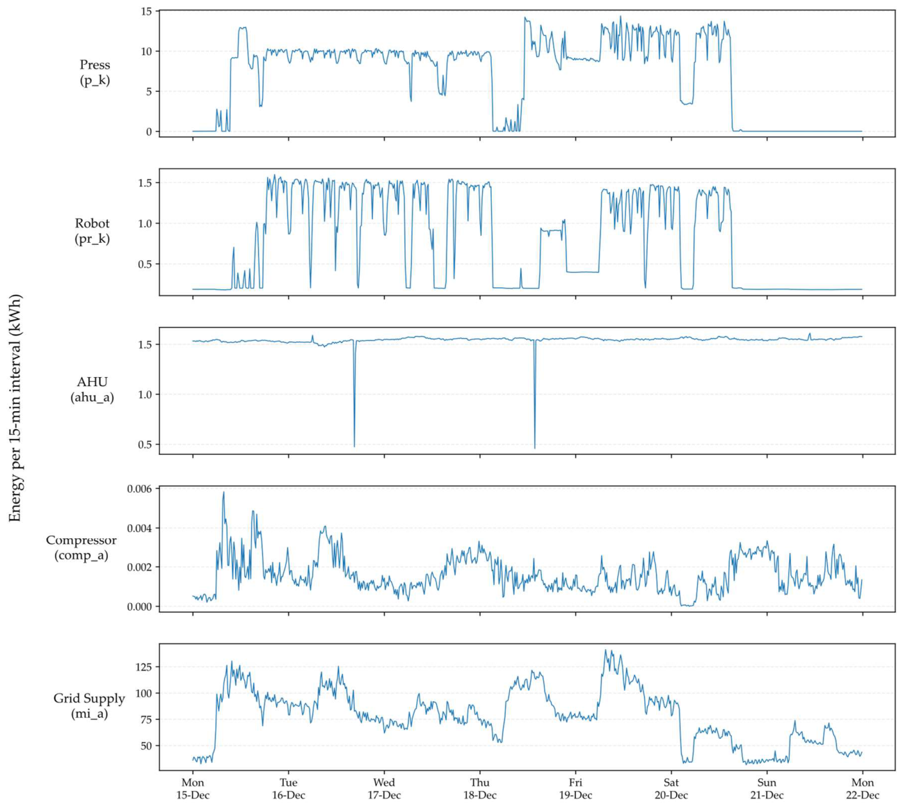
As summarised in

Table 4. Summary statistics of the released Gold-layer dataset (ALL phase).

Metric	Value
Number of assets	43
Time span (UTC)	31 December 2024 07:30 to 31 December 2025 23:45
Temporal resolution	15 min
Total ALL-phase windows	1,039,873
Total measured energy	2.96 GWh
Mean data coverage	99.99%
Median data coverage	100.00%
Mean reliable coverage	97.87%
Median reliable coverage	100.00%
Reliable ALL-phase windows	97.72%

, the publicly released Gold layer contains 4,103,703 rows when all phase-level representations are included and 1,039,873 rows when restricted to the synthetic ALL phase intended for asset-level comparative analysis. The dataset covers 43 distinct monitored assets and 172 distinct asset-phase streams over a one-year period from 31 December 2024 07:30 UTC to 31 December 2025 23:45 UTC. Across the ALL-phase representation, the published dataset contains 2.96 GWh of measured electrical energy. Mean data coverage is 99.99%, median data coverage is 100.00%, mean reliable coverage is 97.87%, and 1,016,182 of 1,039,873 ALL-phase windows (97.72%) satisfy the reliability criterion. These statistics indicate that the released dataset is both longitudinally extensive and highly complete despite being derived from heterogeneous retrofit industrial telemetry. These results reflect the robustness of the acquisition system and the effectiveness of the data quality handling procedures described in Section 3. Together, these metrics demonstrate that the dataset provides extensive temporal coverage and high-quality observations suitable for downstream analytical tasks. Because the released dataset includes meters at multiple hierarchical levels (e.g., supply, distribution, and asset-level sub-metering), aggregate energy summed across all published meters is not directly comparable to whole-site billed consumption. Total energy values reported for the released dataset therefore describe cumulative metered energy across the monitoring hierarchy rather than a single net site import measurement. Figure 6 highlights clear differences in load behaviour across asset types under live industrial conditions. The press and robot exhibit intermittent, production-driven demand with distinct duty cycles, while the AHU shows a relatively stable base load with minor disturbances. The compressor displays variable, load-dependent cycling behaviour, and the grid supply reflects the aggregate impact of these interacting subsystems over time.

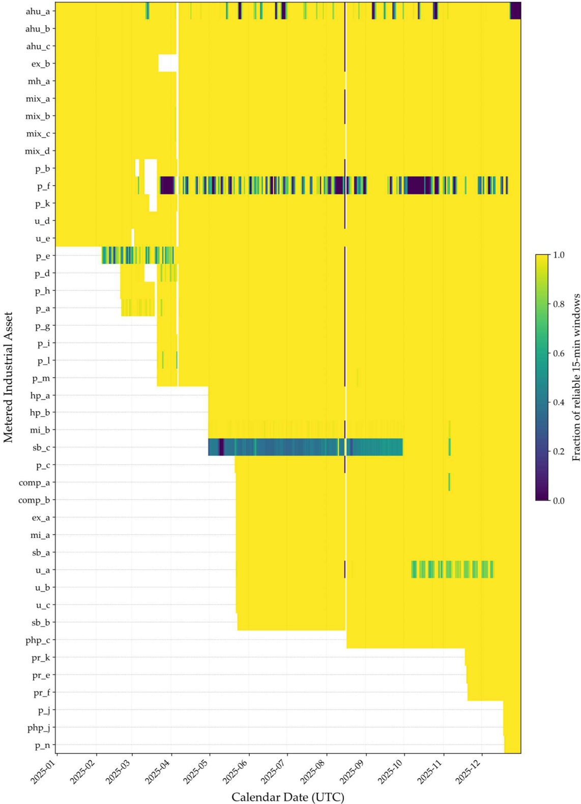
Figure 7 presents a heatmap of daily reliability across all monitored assets (Phase = ALL), where each row corresponds to an individual asset and each column to a calendar date. Colour intensity represents the fraction of reliable 15 min windows per day. The predominance of high-reliability regions across assets indicates that data completeness is consistently maintained over time, while localised reductions correspond to commissioning phases, communication interruptions, and documented instrumentation events.

While the reliability results of this study demonstrated strong temporal coverage and reliability, they do not, by themselves, guarantee structural consistency across the monitored hierarchy. To evaluate the internal consistency of the dataset, a topology verification analysis was performed on the ALL-phase Gold layer using parent–child containment tests, parent-group closure checks, and cross-meter correlation analysis. In total, 66 declared parent–child relationships were evaluated. Of these, 21 relationships exhibited zero hard containment violations, and a further 23 showed violation rates below 0.1%, indicating strong consistency for a subset of the monitored hierarchy. However, a number of relationships exhibited substantially higher violation rates, including cases of complete (100%) violation of containment. These deviations are primarily attributable to partial sub-metering coverage, hierarchical aggregation effects, and the presence of distributed generation, rather than systematic errors in instrumentation. Parent-group closure tests similarly indicate that strict hierarchical consistency is not universally satisfied across the dataset. This is expected in retrofit industrial monitoring contexts, where distribution boundaries are only partially instrumented and energy flows may not be fully observable at all hierarchy levels. This result has important implications for downstream use of the dataset. Specifically, the presence of partial sub-metering and incomplete hierarchical observability means that the dataset should not be treated as a closed or fully balanced energy system. Accordingly, it is not suitable as a benchmark for methods that assume strict energy conservation across fully observed hierarchical boundaries, such as idealised energy disaggregation or load decomposition models. Instead, the dataset is more appropriately used for evaluating analytical methods under realistic industrial conditions, where incomplete instrumentation, partial observability, and measurement uncertainty are inherent features of the system.

Cross-meter correlation analysis supports several inferred parent–child relationships consistent with the documented topology, including high-confidence associations such as u_e with sb_b, sb_a with mi_a, and ex_a with sb_a. These relationships exhibit strong correlation and low violation rates, providing statistical support for key portions of the monitoring structure. It is important to note that these validation procedures provide statistical consistency checks rather than definitive proof of electrical topology, as they are based on magnitude-only, interval-aggregated data and cannot resolve bidirectional power flow or unmetered intermediate loads. A complementary validation was performed on the solar distribution subnetwork using raw signal correlation and balance model analysis across the photovoltaic generation meter (mi_b), solar distribution meter (sb_c), grid import meter (mi_a), and downstream heat pump loads (hp_a, hp_b). This analysis evaluates whether the observed behaviour of the solar distribution meter is consistent with a physically meaningful supply–demand boundary rather than a strict hierarchical containment relationship. Across the full observation period, the strongest agreement was obtained for a balance model in which the solar distribution meter reading is consistent with representing the net power flow at that boundary, approximated as downstream heat pump demand minus photovoltaic generation, where generation is treated as negative demand under the adopted sign convention. This model exhibits high correlation (ρ ≈ 0.98) and low residual error relative to alternative formulations. Competing models, including inverse or additive formulations, show substantially poorer agreement and, in some cases, strong negative correlation, indicating incorrect directional assumptions. Conditioned analyses further support this interpretation. During periods of active photovoltaic generation, the same relationship remains dominant, with strong correlation (ρ ≈ 0.95) despite increased residual variability attributable to fluctuating solar input. During night periods, when photovoltaic contribution is negligible, the solar distribution signal closely aligns with aggregate heat pump demand alone, with near-unity correlation (ρ ≈ 0.99) and minimal residual error. These results indicate that the solar distribution meter behaves as a net boundary measurement reflecting the interaction between local generation and downstream consumption. However, consistent with the broader topology validation, this analysis provides statistical and physical coherence rather than strict structural proof, as magnitude-only signals cannot resolve full energy flow directionality or unmetered intermediate loads.

In addition to the quantitative coverage and reliability metrics reported above, the dataset includes a set of explicitly documented instrumentation and configuration issues observed during the monitoring campaign. These issues were identified through a combination of engineering inspection, commissioning records, and retrospective data validation. The documented issues reflect common failure modes encountered in retrofit industrial energy monitoring deployments and include, but are not limited to:

• Reversed current transformer (CT) polarity;
• Misaligned phase references;
• CT ratio misconfiguration;
• Tag or channel misconfiguration within the SCADA system, and;
• Intermittent loss of meter power or communication.

Each issue is recorded as a time-bounded event associated with a specific asset, with defined inception and rectification timestamps. This enables precise identification of affected intervals without requiring inference from the time series alone. From a data quality perspective, these issues fall into two broad categories:

• Magnitude-affecting faults, such as CT polarity reversal or ratio misconfiguration, which may invalidate the physical interpretation of measured power and energy values during the affected period;
• Continuity-affecting faults, such as communication interruptions or temporary power loss, which preserve physical validity but reduce temporal completeness.

2.8. Data Availability and Resuse Notes

The dataset is publicly available through an open access research data repository and is released under a permissive licence to support reuse in energy analytics, industrial informatics, and operational efficiency research. All identifiers have been anonymised at the asset level, and no commercially sensitive production metrics are included. Electrical measurements are provided at a temporal resolution suitable for load profiling, demand analysis, and method benchmarking, but are not intended for real-time control or billing applications. The released dataset is distributed primarily in columnar Parquet format, with mirrored CSV exports also provided to support accessibility across a wider range of analytical environments. CSV files were generated directly from the released Gold-layer Parquet partitions and validated for equivalence using partition-level checks on row counts, column ordering, non-floating-point equality, and floating-point consistency within a defined numerical tolerance. The decision to release only interval-aggregated data reflects a deliberate balance between scientific transparency and responsible industrial data governance. While high-frequency telemetry was used internally for quality control and validation, sub-minute operational signatures may encode sensitive production characteristics. The corresponding processing procedures are described in Section 3. The 15 min aggregation interval preserves analytical utility for energy modelling, benchmarking, and method development while mitigating exposure of fine-grained operational behaviour. Users should consider the documented logging cadence, timing variability, and data quality flags when applying resampling, forecasting, or machine learning techniques. The documented medallion architecture provides a transparent processing framework, enabling researchers to understand and reproduce the transformations applied to the released dataset.

3. Methods

3.1. Source Data and Bronze Layer Definition

The dataset is derived from electrical measurements logged by an industrial SCADA system originated by a heterogeneous fleet of energy meters and stored in an SQL historian. For analytical reproducibility, these historian tables were periodically exported to columnar Parquet files, with each file corresponding to a single metered asset and containing timestamped, wide-format electrical quantities. These SQL-to-Parquet exports constitute the Bronze layer of the dataset. No transformations, filtering, interpolation, or quality screening were applied at this stage. The exported files preserve the original temporal ordering, native measurement resolution, and register-level values as recorded by the SCADA environment. Once generated, Bronze files were treated as immutable inputs to downstream processing. This design ensures that all downstream transformations remain fully traceable to original SCADA measurements, supporting auditability and reproducibility in industrial analytics workflows.

3.2. Silver Layer Construction: Normalisation, Quality Flags, and Partitioning

The Silver layer constitutes the first structured transformation stage of the medallion architecture. This stage’s purpose is to convert heterogeneous SCADA-derived meter exports into a temporally coherent, analysis-ready telemetry representation while preserving auditability and traceability to original measurements. Processing was implemented in Python 3.13 [21] using the Polars dataframe engine to enable deterministic, columnar transformations and efficient incremental execution. No interpolation, smoothing, or temporal resampling was performed at the Silver stage. All numeric quantities were stored as 64-bit floating-point values (Float64) to preserve measurement precision during downstream aggregation. All operations were applied consistently across assets, with configuration-based overrides where required. The design outlined below ensures that all derived fields and quality indicators remain directly traceable to original SCADA observations, supporting auditability in downstream analyses.

• Timestamp Handling and Time Zone Normalisation: Each source file contains a timestamp column (‘CreatedOn’) generated by the SCADA system’s SQL database. Where timestamps were stored as local, time zone-naïve values, they were interpreted using a site-specific default time zone (Europe/Dublin) and converted to UTC. Ambiguous or non-existent local timestamps arising from daylight-saving transitions were resolved using a conservative forward-shift strategy. All downstream processing was performed using UTC timestamps (‘CreatedOnUtc’).
• Reshaping from Wide to Long Format: Raw exports store per-phase electrical quantities in wide format (e.g., ‘L1_PWR_ACTV’, ‘L2_CRNT’). These records were reshaped into a long format, producing one row per (‘AssetId’, ‘Phase’, ‘CreatedOnUtc’) combination. Phase identifiers were standardised to {‘L1’, ‘L2’, ‘L3’}, enabling consistent multi-phase aggregation in later stages.
• Unit Normalisation and Derived Quantities: Active power values were normalised to kilowatts (kW), with per-asset overrides supported via a configuration map where meters are reported in non-standard units. Apparent power (kVA) was taken directly from the meter where available; otherwise, it was derived using the relationship:

  $$S={\displaystyle \frac{P}{PF}}$$

  (1)

  where P is active power and PF is the reported power factor. Power factor values were preserved in raw form and separately clamped only for use in derived calculations, ensuring that implausible readings could be identified without being silently corrected. To preserve measurement fidelity, power factor values were stored in raw form (‘PowerFactor_raw’). A clamped version (‘PowerFactor_clamped’) was generated solely for use in derived calculations, restricting values to the interval [0, 1.1] to avoid numerical instability. This approach prevents silent correction of anomalous readings while enabling stable derivation of apparent power.
• Temporal Differencing and Data Quality Flags: For each (‘AssetId’, ‘Phase’) stream, successive timestamps were differenced to compute inter-arrival times. A configurable gap threshold (300 s) was applied to flag discontinuities. In addition, per-row quality indicators were generated to identify missing values, negative power readings, implausible power factor values, and negative apparent power. A composite binary flag (IsReliableRow) was assigned to each record, indicating whether the row passed all quality checks. These flags were retained explicitly rather than used to discard data, allowing downstream analyses to enforce reliability criteria transparently.
• Row-Level Data Quality Indicators: Rather than filtering suspect observations during ingestion, the Silver layer explicitly encodes quality conditions as binary flags. The following per-row indicators were generated:
  • IsGap: Inter-arrival interval exceeds threshold;
  • IsMissing_Power: Active power unavailable;
  • IsNegative_Power: Negative active power measurement;
  • IsOutlier_PF: Power factor outside physical bounds;
  • IsOutlier_Apparent: Negative apparent power.

A composite reliability indicator (IsReliableRow) was defined as the logical complement of all row-level anomaly conditions. This design preserves the full telemetry record while allowing downstream processes to enforce reliability criteria transparently and reproducibly. Importantly, no rows were removed at the Silver stage solely on the basis of quality flags, although incremental processing filters are applied for execution efficiency during practical execution of the pipeline. Exclusion policies are deferred to higher processing layers where analytical context is available.

6.

Deduplication and Partitioned Storage: Duplicate records were removed based on (AssetId, Phase, CreatedOnUtc) keys, retaining the last encountered observation for each key combination. Silver outputs were written as partitioned Parquet files organised by asset identifier and UTC date (asset_id=…/dt_utc=…). Daily partitions were written idempotently, with affected partitions fully replaced during incremental reprocessing. Incremental execution was supported via per-asset watermarks and a sliding overlap window, ensuring late-arriving or corrected source data were consistently reconciled without requiring full dataset rebuilds.

3.3. Gold Layer Construction: Fixed Interval Energy Aggregation

The Gold layer constitutes the publicly released dataset. It transforms high-frequency, irregularly sampled Silver telemetry into fixed 15 min interval aggregates suitable for load profiling, benchmarking, forecasting, and operational energy analysis while mitigating exposure of sub-minute operational signatures. Gold generation was implemented in Python using Polars and executed directly over partitioned Silver Parquet files.

3.3.1. Interval Reconstruction and Forward-Hold Model

Silver telemetry provides timestamped active power observations P(t) at an intended SCADA cadence (nominally ~3 s) with non-negligible jitter and intermittent dropouts. To enable deterministic energy integration without resampling, consecutive observations for each (AssetId, Phase) stream were interpreted using a forward-hold assumption: each recorded power value was treated as piecewise constant over the interval until the next observation. For each observation at time t_0, the subsequent timestamp t₁ was obtained by shifting the series forward (i.e., the next recorded sample), forming candidate intervals [t₀, t₁). To prevent bridging across outages or non-physical discontinuities, intervals were retained only when

• t₁ existed and t₁ > t₀;
• (t₁ − t₀) ≤ τ_gap, where τ_gap = 300 s by default.

Intervals exceeding τ_gap were excluded from integration and contributed to reduced coverage metrics rather than being implicitly imputed. No interpolation between samples was performed; energy integration assumes piecewise-constant power between consecutive observations. No attempt was made to estimate or impute energy during telemetry gaps.

3.3.2. Power Magnitude Policy

For most assets, active power values were treated as magnitude-only prior to aggregation, with negative readings clipped to zero at the Gold stage. For assets representing upstream supply, signed power values were retained to preserve net flow directionality; the negative readings for remaining assets were clipped to zero at the Gold stage:

$$P_{\mathrm{e}\mathrm{f}\mathrm{f}}=\max (P,0)$$

This policy reflects the dataset’s intended use as a facility-level energy consumption resource rather than a bidirectional power flow dataset. By enforcing a uniform magnitude representation, aggregation logic remains consistent across suppliers and internal loads, and interval energy is non-negative by construction.

3.3.3. Window Fragmentation at 15-Minute Boundaries

Each valid interval [t0, t1) may intersect one or more 15 min windows. Intervals were therefore fragmented at 15 min boundaries. For each intersected window with start time w, fragment duration was computed as

$${\mathsf{\Delta }t}_{frag}=\max \left(0,\min \left(t_1,w+900\right)-\max \left(t_0,w\right)\right)$$

where times are expressed in UTC and 900 s corresponds to 15 min. Only fragments with Δt_frag > 0 were retained. Fifteen-minute windows were treated as half-open intervals [w,w + 900), preventing double counting at boundaries.

3.3.4. Energy Integration and Interval Statistics

Energy for each fragment was computed using

$$E_{frag}=P_{eff}·{\displaystyle \frac{{\mathsf{\Delta }t}_{frag}}{3600}}$$

where P_eff is the magnitude-adjusted active power (kW). Fragment contribution was summed (AssetId, Phase, window_start_utc) to produce 15 min interval aggregates. Energy integration was performed using double-precision arithmetic; cumulative rounding error over 15 min windows is negligible relative to meter resolution. For each window, the following metrics were calculated:

• Energy_kWh_15m: Total integrated energy (kWh), computed from fragments originating from rows marked as reliable;
• Demand_kW: 4 x Energy_kWh_15m, equivalent to mean interval power;
• AvgPower_kW_15m: duration-weighted mean power using reliable fragments only.

As power is treated as non-negative magnitude, all interval energy and demand values are non-negative by design.

3.3.5. Coverage and Reliability Metrics

Energy and mean power metrics are derived from reliable fragments, while coverage metrics reflect both total observed and reliable durations. To quantify data completeness, coverage metrics were derived directly from fragment durations:

• SecondsObserved: Total observed seconds within the window (capped at 900);
• SecondsReliable: Observed seconds originating from Silver rows marked reliable (capped at 900);
• DataCoveragePct: $100\times SecondsObserved/900$;
• ReliableCoveragePct: $100\times SecondsReliable/900$.

A binary window-level reliability flag (IsReliableWindow) was defined using a configurable threshold (default θ = 0.8):

$$IsReliableWindow=1[SecondsReliable\ge 900\theta ]$$

Incomplete windows are retained in the dataset, with coverage explicitly reported, enabling sensitivity analysis rather than silent exclusion.

3.3.6. Phase Aggregation

Per-phase records (L1, L2, L3) were aggregated to a synthetic ALL phase representing total asset-level consumption. Energy and demand were summed across phases. Mean power for the ALL phase was computed as a seconds-weighted average using reliable fragment durations to mitigate bias arising from unequal phase coverage.

3.3.7. Day Boundary Continuity and Incremental Generation

As Silver partitions are written by UTC date, the final observation of a given day may close into the first timestamp of the subsequent day. To prevent truncation bias at day boundaries, the first timestamped row per phase from the following day was temporarily appended during processing. After aggregation, only windows whose start time fell within the target UTC date were written, ensuring idempotent daily output without double counting. Gold outputs were written as partitioned Parquet files using Hive-style directory structure (asset_id=…/dt_utc=…). A deterministic overwrite policy ensures reproducibility during incremental regeneration.

3.3.8. Handling of Documented Instrumentation Faults

Exclusion rules were applied only in cases where measurement magnitude was known to be structurally invalid (e.g., incorrect tag mapping or CT ratio misconfiguration). Faults affecting continuity (e.g., power supply interruption) were handled implicitly through gap detection and coverage metrics rather than explicit row removal. These exclusions were restricted to periods for which magnitude integrity could not be guaranteed. Affected windows remain represented in the dataset via reduced coverage metrics rather than imputation.

3.4. Known Dataset Limitations

This dataset reflects engineering design choices intended to balance reproducibility, transparency, and analytical usability. The following structural limitations should be considered by downstream users.

3.4.1. Sampling Irregularity and Forward-Hold Integration

Power measurements originate from a SCADA system with an intended cadence of approximately 3 s, though actual inter-arrival intervals vary. Energy integration at the Gold stage assumes piecewise-constant power between consecutive observations (forward-hold model). No interpolation or smoothing is performed. Consequently, intra-interval power variation occurring between samples is not explicitly resolved.

3.4.2. Telemetry Gaps and Non-Imputation

Intervals exceeding the configured gap threshold (300 s) are excluded from energy integration rather than interpolated. Energy during telemetry outages is not estimated. Instead, coverage metrics are provided at both row and window levels. Users performing statistical or forecasting analyses should consider coverage percentages and reliability flags when selecting windows for analysis, particularly in statistical or forecasting applications.

3.4.3. Magnitude-Only Representation

Active power values in the published dataset are primarily represented as non-negative magnitude, with negative readings clipped to zero for most assets prior to aggregation. For assets representing upstream supply, signed power values are retained to preserve net flow directionality. As a result, the dataset is not suitable for bidirectional power flow analysis, export quantification, or regeneration studies.

3.4.4. Instrumentation Fault Periods

Documented instrumentation faults that were found to have structurally invalidated the magnitude of power measurements (e.g., incorrect tag mapping or CT ratio misconfiguration) were excluded via time-bounded filtering prior to aggregation. Faults affecting measurement continuity (e.g., power supply interruptions) are represented implicitly through reduced coverage rather than explicit correction. No retrospective recalibration or scaling adjustments were applied.

3.4.5. Temporal Resolution

The publicly released dataset provides fixed 15 min aggregates. Sub-minute load transients and short-duration peak events are averaged within this window and therefore not directly observable.

3.4.6. Site-Specific Context

The dataset reflects measurements from a single industrial facility with site-specific asset configurations, load profiles, and SCADA architecture. While the processing pipeline is generalisable, the load characteristics themselves should not be assumed to represent broader industrial populations without further validation. This design choice also limits strict electrical topology inference in the presence of distributed generation, since photovoltaic offset can reduce measured upstream grid import without reducing downstream gross load demand. The staggered commissioning of metering infrastructure reflects realistic deployment conditions in retrofit industrial monitoring environments and provides a heterogeneous temporal structure that is valuable for evaluating methods under partial observability. These limitations are intentionally exposed rather than mitigated, enabling downstream users to apply context-specific assumptions and analytical constraints.

References

1. Cosgrove, J.; Duarte, M.-J.R.; Littlewood, J.; Wilgeroth, P. An Energy Mapping Methodology to Reduce Energy Consumption in Manufacturing Operations. Proc. Inst. Mech. Eng. Part B J. Eng. Manuf. 2018, 232, 1731–1740. [Google Scholar] [CrossRef]
2. May, G.; Barletta, I.; Stahl, B.; Taisch, M. Energy Management in Production: A Novel Method to Develop Key Performance Indicators for Improving Energy Efficiency. Appl. Energy 2015, 149, 46–61. [Google Scholar] [CrossRef]
3. Miller, C.; Kathirgamanathan, A.; Picchetti, B.; Arjunan, P.; Park, J.Y.; Nagy, Z.; Raftery, P.; Hobson, B.W.; Shi, Z.; Meggers, F. The Building Data Genome Project 2, Energy Meter Data from the ASHRAE Great Energy Predictor III Competition. arXiv 2020. [Google Scholar] [CrossRef] [PubMed]
4. Xu, H.; Yu, W.; Griffith, D.; Golmie, N. A Survey on Industrial Internet of Things: A Cyber-Physical Systems Perspective. IEEE Access 2018, 6, 78238–78259. [Google Scholar] [CrossRef] [PubMed]
5. Navarro, V.M.; Barragán, M.; Nieto, R.; Ureña, J.; Hernández, Á. HIFDA-High-Frequency Electrical Voltage and Current Signals from Household Appliances. Sci. Data 2025, 12, 527. [Google Scholar] [CrossRef] [PubMed]
6. Khasawneh, H.J.; Asbahi, R.A.; Alzariqi, A.W.; Qada, D.R.A.; Bujuk, A.; Nawfal, M.A.; Tareen, M. Industrial IoT-Based Submetering Solution for Real-Time Energy Monitoring. Discov. Internet Things 2025, 5, 15. [Google Scholar] [CrossRef]
7. Weyer, S.; Schmitt, M.; Ohmer, M.; Gorecky, D. Towards Industry 4.0-Standardization as the Crucial Challenge for Highly Modular, Multi-Vendor Production Systems. IFAC-Pap. 2015, 48, 579–584. [Google Scholar] [CrossRef]
8. Bunse, K.; Vodicka, M. Managing Energy Efficiency in Manufacturing Processes–Implementing Energy Performance in Production Information Technology Systems. In IFIP International Federation for Information Processing/IFIP; Springer: Berlin/Heidelberg, Germany, 2010; pp. 260–268. [Google Scholar] [CrossRef]
9. Garcia, F.D.; Souza, W.A.; Diniz, I.S.; Marafão, F.P. NILM-Based Approach for Energy Efficiency Assessment of Household Appliances. Energy Inform. 2020, 3, 10. [Google Scholar] [CrossRef]
10. Batini, C.; Cappiello, C.; Francalanci, C.; Maurino, A. Methodologies for Data Quality Assessment and Improvement. ACM Comput. Surv. 2009, 41, 1–52. [Google Scholar] [CrossRef]
11. Alarcón, M.; Martínez-García, F.M.; De León Hijes, F.C.G. Energy and Maintenance Management Systems in the Context of Industry 4.0. Implementation in a Real Case. Renew. Sustain. Energy Rev. 2021, 142, 110841. [Google Scholar] [CrossRef]
12. Javied, T.; Rackow, T.; Stankalla, R.; Sterk, C.; Franke, J. A Study on Electric Energy Consumption of Manufacturing Companies in the German Industry with the Focus on Electric Drives. Procedia CIRP 2016, 41, 318–322. [Google Scholar] [CrossRef]
13. Weidmüller. EM220 Series Three-Phase Energy Meter Data Sheet. Weidmüller Interface GmbH & Co. KG. 2026. Available online: https://datasheet.weidmueller.com/pdf/en/7760051005/scope/2/ (accessed on 28 February 2026).
14. Rayleigh Instruments Ltd. RI-F200 Series Energy Meter Technical Specification. 2026. Available online: https://www.rayleigh.com/media/uploads/RI_Data_Sheet_RI-F200_W_05_12_19.pdf (accessed on 28 February 2026).
15. Rayleigh Instruments Ltd. RI-F400 Series Energy Meter Technical Specification. 2026. Available online: https://www.rayleigh.com/media/uploads/RI_Data_Sheet_RI-F400_W_19_08_19.pdf (accessed on 28 February 2026).
16. Modbus Organization. Modbus Application Protocol Specification V1.1b3. 2012. Available online: https://www.modbus.org/file/secure/modbusprotocolspecification.pdf (accessed on 28 February 2026).
17. X2 Pro 10 10” HMI with IX Runtime Module Datasheet. Beijer Electronics AB. 2026. Available online: https://icdn.tradew.com/file/201606/1569362/pdf/7271807.pdf (accessed on 28 February 2026).
18. Box2 Pro Installation Manual. Beijer Electronics AB. 2023. Available online: https://www.beijerelectronics.com/docs/BoX2-pro-Installation/BoX2_pro_Installation_MAEN275_2023-09-19.pdf (accessed on 28 February 2026).
19. Mitsubishi Electric. MELSEC Communication Protocol Reference Manual (MC Protocol). 2026. Available online: https://dl.mitsubishielectric.com/dl/fa/document/manual/plc/sh080008/sh080008ab.pdf (accessed on 28 February 2026).
20. Weidmüller GTI Software GmbH. PROCON-WEB Online Documentation. 2024. Available online: https://support.weidmueller.com/online-documentation/latest/293445/files/HilfeSystem/HilfeSystem.html (accessed on 28 February 2026).
21. Python Software Foundation. Python Release Python 3.13.0. 2024. Available online: https://www.python.org/downloads/release/python-3130/ (accessed on 28 February 2026).
Figure 1. High-level electrical distribution and sub-metering architecture of the study facility, illustrating generation sources, distribution boards, major load groups, and the placement and communication types of energy meters.
Data 11 00101 g001
Figure 2. Schematic representation of the standardised EMS cabinet design used across all monitored assets, showing separation of voltage references, CT terminations, protective devices, and communication interfaces. Arrows above the CT terminals indicate CT connection orientation, while arrows on the disconnect terminals reflect switch operation markings.
Data 11 00101 g002
Figure 3. (Left) Typical retrofit energy monitoring cabinet installed at asset level, housing a three-phase energy meter, voltage references, and current transformer terminations. (Right) Internal layout of a standardised EMS cabinet, illustrating CT termination, voltage reference protection, and isolation components used to ensure safe and repeatable retrofit installation.
Data 11 00101 g003
Figure 4. (Left) Communication network topology routes for energy meter data acquisition, showing direct Modbus TCP/IP connections and indirect PLC- and gateway-mediated pathways to the SCADA IPC. (Above Right) IIoT-enabled HMI for local machine monitoring and control. (Below Right) IIoT gateway with serial Modbus RTU adapter connected to a network switch via Ethernet, enabling integration of legacy devices into the SCADA network.
Data 11 00101 g004
Figure 5. (Left) End-to-end data acquisition and processing architecture showing SCADA-based acquisition, SQL historian archiving, and Bronze–Silver–Gold data transformation pipeline. (Above Right) SCADA dashboard view illustrating real-time energy monitoring across production and utility zones. (Middle Right) SCADA tag configuration interface showing mapping of electrical measurement variables (e.g., current, voltage, active power, power factor). (Below Right) Example SQL historian export in wide-format structure, preserving raw timestamped measurements prior to transformation.
Data 11 00101 g005
Figure 6. Multi-panel time-series view of selected assets over a representative operational week. Panels are stacked vertically, with each horizontal panel corresponding to a distinct asset (press, robot, AHU, compressor, and grid supply).
Data 11 00101 g006
Figure 7. Heatmap showing the daily fraction of reliable 15 min windows for each asset (Phase = ALL). Rows correspond to individual metered assets and columns to calendar dates. Colour intensity represents the fraction of reliable windows, indicating overall data completeness and localised periods of reduced coverage.
Data 11 00101 g007