Modelling Extreme Losses in JSE Life Insurance Price Index Growth Rates Using the Generalised Extreme Value Distribution (GEVD) and the Generalised Pareto Distribution (GPD)

Abstract

The life insurance sector plays a critical role in financial system stability but is inherently exposed to extreme market fluctuations due to long-term liabilities and asset–liability mismatches. This study investigates extreme losses in the growth rates of the JSE Life Insurance Price Index (LIPI) using the Generalised Extreme Value Distribution (GEVD) and the Generalised Pareto Distribution (GPD) under the Extreme Value Theory (EVT) framework. Monthly data from January 2000 to October 2023 were transformed into a loss series, and extreme events were captured using quarterly block maxima and a POT threshold at the 95th percentile. Model parameters were estimated through Maximum Likelihood Estimation, and downside risk was assessed using return levels, Value-at-Risk (VaR), and Tail Value-at-Risk (tVaR). The GEVD model produced a negative shape parameter, consistent with a bounded Weibull-type tail, while the GPD indicated a heavy-tailed distribution. Return level estimates show escalating loss magnitudes and widening uncertainty over longer horizons, reflecting the challenges of projecting rare events. Kupiec backtesting confirms the adequacy and reliability of the GEVD-based VaR across all confidence levels, whereas the GPD underestimates risk at lower thresholds. These findings indicate significant tail risk within the South African life insurance equity segment and underscore the importance of EVT-based risk measures for capital planning and regulatory oversight. The study contributes to financial risk modelling in the life insurance sector and offers practical insights for strengthening solvency assessment and enterprise risk management frameworks.

1. Introduction

The financial sector plays a pivotal role in economic growth by facilitating investment, risk management, and wealth accumulation. Within this sector, the life insurance market contributes significantly by providing long-term financial security, mobilising household savings, and supporting capital formation [1]. Life insurers collect premiums and allocate them to long-term investments, acting as major institutional investors and thereby enhancing financial market development and stability [2]. Empirical evidence from developing countries further suggests that the expansion of life insurance markets is positively associated with financial stability, particularly bank stability, underscoring its role in strengthening overall financial system resilience and economic sustainability [3].

The life insurance sector is also uniquely exposed to financial market shocks due to its management of long-term liabilities, which require careful asset–liability matching. This exposure was particularly evident during the COVID-19 pandemic, which caused significant market volatility and heightened mortality risk, placing additional stress on insurers’ financial positions in some cases. Life insurers’ liabilities are often more sensitive to interest rate and market fluctuations than their assets, creating potential vulnerabilities under such extreme conditions [4]. The combination of long-term liabilities, potential asset–liability mismatches, and exposure to market risk makes life insurers particularly susceptible to negative returns on market indices, which can signal stress, solvency challenges, and broader financial instability. Monitoring indicators of insurance stress is therefore crucial, as insurers’ financial positions are closely linked to macroeconomic and market conditions, and systemic risk indices can provide early warning signals and inform regulatory responses.

The financial sector serves as a critical engine of economic development by efficiently allocating funds from surplus units to deficit units, thereby promoting investment and growth [5]. Financial markets are often regarded as a “barometer” of a country’s economic health [6]. The Johannesburg Stock Exchange (JSE), established in 1887, is the largest stock exchange in Africa and plays a vital role in price discovery, risk management, and capital mobilisation [7]. However, the global financial landscape has been characterised by recurrent episodes of instability, including the Asian Financial Crisis (1997–1998), the Global Financial Crisis (2007–2008), the Chinese Stock Market Crash (2015–2016), and the COVID-19 pandemic, all of which have highlighted the vulnerability of financial systems to extreme shocks [8].

In South Africa, research applying Extreme Value Theory (EVT) has predominantly focused on broad financial market indices, with relatively few studies examining sub-sectors such as the life insurance price indices. Empirical evidence shows that EVT methods, particularly the Peak-Over-Threshold (POT) and the Block Maxima (BM) approaches to selecting extremes, have been used to model extreme returns and improve risk measures such as Value-at-Risk (VaR) and Expected Shortfall (ES) for the JSE index. These studies highlight the advantages of tail-focused modelling over traditional approaches that rely on normality assumptions [9].

Traditional risk management models, which are largely based on the Normal (Gaussian) distribution, have been widely criticised for their inability to adequately capture rare but high-impact extreme events [10]. Financial return series often exhibit fat tails and volatility clustering, leading to the underestimation of risk when conventional models are applied [11]. As a result, EVT has emerged as a robust statistical framework for modelling the tail behaviour of financial returns. EVT focuses specifically on extreme observations and provides a more accurate estimation of risk measures in the tails of the distribution. The Generalised Extreme Value Distribution (GEVD), used under the BM approach, and the Generalised Pareto Distribution (GPD), used under the POT approach, enable more reliable estimation of extreme losses, including VaR and ES [12].

The relevance of EVT in this context stems from the inherent characteristics of financial markets, which are marked by volatility, uncertainty, and the potential for extreme losses. Return distributions typically exhibit heavy tails and volatility clustering, invalidating the assumption of normality [12]. Although extreme market movements occur infrequently, they carry disproportionately large economic consequences for investors, insurers, regulators, and policymakers. Consequently, modelling tail behaviour has become a central concern in modern financial econometrics and risk management. EVT provides a powerful framework for analysing financial markets under exceptionally optimistic or pessimistic conditions, as it allows the quantification of stochastic behaviour at unusually large or small levels, thereby enabling the estimation of probabilities for events more extreme than those previously observed [13].

The primary aim of this study is to model and quantify extreme losses in the growth rates of the JSE LIPI using EVT. The study applies the GEVD under the BM approach and complements it with the GPD under the POT approach. Integrating both approaches provides a comprehensive analysis of tail risk, enhancing the accuracy and robustness of extreme risk estimation in the South African life insurance sector. Accordingly, this study seeks to answer the following research question: How can the GEVD and GPD be applied to quantify and understand extreme losses in the South African life insurance equity market?

2. Literature Review

The insurance industry is inherently exposed to extreme and unpredictable losses, often resulting in non-stationary claim and return series. Empirical evidence shows that insurance data exhibit volatility clustering, seasonality, and sensitivity to rare but severe events. Ref. [14] found that motor insurance claim settlements were highly volatile and influenced by seasonal patterns, with extreme claims concentrated toward the end of the year. Ref. [10] demonstrated that traditional statistical models were inadequate for capturing large losses in fire insurance, thereby motivating the application of EVT to model tail behaviour more effectively. These characteristics reflect the structural nature of insurance markets, which are driven by long-term liabilities, exposure to catastrophic risks, and regulatory capital requirements. As a result, accurate modelling of extreme losses is critical for solvency assessment and risk management in the insurance sector.

In financial markets, large-scale shocks such as the global financial crisis and the COVID-19 pandemic have revealed that sectoral responses are heterogeneous. Ref. [15] showed that during the COVID-19 pandemic, the Hong Kong financial market exhibited increased financial connectedness, with higher network density and clustering in partial correlation networks compared to previous financial crises, indicating heightened systemic risk. More recent evidence by [11] indicates that the financial sector index exhibits significantly higher tail risk compared to the industrial sector, particularly during periods of market stress. These findings highlight the importance of sector-specific modelling of extreme losses, especially for indices such as the LIPI, which may exhibit distinct risk dynamics due to the nature of insurance liabilities and market exposure. This underscores the need to move beyond aggregate market indices and focus on sector-level behaviour when assessing extreme risk.

Ref. [12] analysed how extreme events are modelled in South African financial markets using EVT. They used five years of daily data from the JSE All-Share Total Return Index (ALSTRI) and the USD/ZAR exchange rate to compare the BM method, which fits the GEVD), with the POT approach, which fits the GPD. Their results show that the 100-year return levels from the BM method are close to the historical maxima, whilst the POT method yielded higher estimates of return levels. The study demonstrates that the GEVD approach provides stable, consistent, and meaningful long-term risk measures when modelling block maxima. Despite methodological differences, the authors affirm the robustness and practical relevance of GEVD for modelling tail behaviour in financial data.

Similarly, [16] analysed extreme-value models for the JSE Mining Index, focusing on negative returns. Recognising the inadequacy of classical normality assumptions for leptokurtic financial data, the study employed both GEVD and GPD approaches, using Maximum Likelihood Estimation (MLE) and Probability-Weighted Moments (PWM). Their findings indicate that EVT-based models outperform the normal distribution in estimating Value-at-Risk (VaR), with GEVD capturing larger maxima and GPD providing more conservative estimates for capital adequacy. However, the study highlights practical challenges in selecting appropriate block sizes and thresholds, which can significantly influence model outcomes.

A wide range of EVT-based approaches has been applied in modelling extreme financial risks. The POT method, combined with the GPD, is widely used to model exceedances over high thresholds. Ref. [8] applied this approach to JSE industrial index returns and found evidence of bounded losses, suggesting asymmetry between extreme gains and losses. Ref. [17] extended the POT framework by incorporating the extremal index to account for clustering in extreme events, showing that ignoring such dependence can lead to underestimation of VaR and ES.

Alternatively, the BM approach models the maximum loss within fixed intervals using the GEVD. Ref. [11] applied this method to JSE indices and found differing tail behaviours across sectors, with the financial index exhibiting heavy-tailed characteristics while the industrial index displayed bounded extremes. These findings suggest that different sectors require varying levels of risk capital due to their exposure to extreme losses. Recent methodological advancements have further extended EVT applications. For example, [12] introduced the Blended GEVD (bGEVD), which combines features of multiple extreme value distributions to improve flexibility in capturing tail behaviour. Their results indicate that such hybrid models can enhance short-term forecasting of extreme events in financial time series.

Previous research highlights the effectiveness of the GEVD in enhancing risk assessment, pricing decisions, and regulatory compliance in the insurance industry by accurately capturing extreme outcomes across datasets and regions. In this study, the GEVD is applied to the JSE Life Insurance Price Index (LIPI) to extend the use of EVT in evaluating financial performance risk, providing empirical estimates of extreme losses through VaR and tVaR for the South African life insurance sector. The GEVD is particularly suitable for modelling extreme losses due to its ability to capture tail behaviour more effectively than traditional distributions. Furthermore, the BM approach ensures independence in the selected extremes, unlike the POT approach, which may introduce serial dependence or autocorrelation in exceedances.

Although hybrid models such as the blended bGEVD offer increased flexibility in capturing complex tail behaviour, their empirical application remains limited and lacks widespread validation in financial risk modelling, particularly in emerging market contexts. Moreover, such models often require larger sample sizes and involve more complex estimation procedures, which may not be suitable for datasets characterised by limited extreme observations. In contrast, the classical GEVD and GPD provide parsimonious, theoretically grounded, and widely applied frameworks that are consistent with EVT and extensively used in actuarial and financial risk modelling. Consequently, this study adopts the GEVD and GPD to ensure robustness, interpretability, and comparability with existing empirical literature.

Despite these developments, several gaps remain in the literature. From a theoretical perspective, the application of more advanced EVT-based models in financial and insurance contexts remains limited, with most studies continuing to rely on the classical GEVD and GPD frameworks. Methodologically, many studies assume independence in financial returns, despite strong evidence of clustering in extreme events, highlighting the need for models that incorporate dependence structures. Empirically, while various Johannesburg Stock Exchange (JSE) indices, such as the All-Share and Financial indices, have been extensively studied, there is a lack of research specifically focusing on the Life Insurance Price Index (LIPI). Given the unique characteristics of the insurance sector, particularly its exposure to long-term liabilities and systemic shocks, this represents an important gap in the literature.

To address these gaps, this study applies the GEVD to model extreme losses in JSE LIPI growth rates and complements this approach with the GPD. Focusing on the life insurance sector and comparing the BM and POT approaches contributes to the empirical literature on extreme value modelling and provides valuable insights into tail risk relevant for actuarial practice and financial risk management.

3. Methodology

To model extreme losses in the growth rates of the Life Insurance Price Index (LIPI), the Generalised Extreme Value Distribution (GEVD) is employed. Unlike typical analysis that focuses on overall or growth, this study specifically targets the lower tail of the distribution to capture severe negative movements. Extreme observations are identified using the Block Maxima (BM) approach. The approach partitions the dataset into non-overlapping blocks and selects the minimum growth rate in each block.

The GEVD parameters are estimated using Maximum Likelihood Estimation (MLE), which optimises the likelihood function at the observed minima [18]. Risk measures, including Value at Risk (VaR) and Tail Value at Risk (tVaR), are calculated to quantify potential extreme monthly loss within a quarter in LIPI growth rates. The model’s effectiveness is assessed via backtesting, evaluating the reliability of VaR and tVaR in capturing rare but severe negative events.

Given that $z_t$ denotes the LIPI at time $t$, the growth rate $\left(y_t\right)$ is now defined as:

$${\mathrm{y}}_{\mathrm{t}}={\displaystyle \frac{{\mathrm{z}}_{\mathrm{t}}}{{\mathrm{z}}_{\mathrm{t}-1}}}$$

(1)

To focus on losses, we transform the growth rates into positive values using:

$${\mathrm{L}}_{\mathrm{t}}=\mathrm{p}\mathrm{o}\mathrm{s}\mathrm{i}\mathrm{t}\mathrm{i}\mathrm{v}\mathrm{e}\left(1-{\mathrm{y}}_{\mathrm{t}}=1-{\displaystyle \frac{{\mathrm{z}}_{\mathrm{t}}}{{\mathrm{z}}_{\mathrm{t}-1}}}\right).$$

(2)

Let $L_1, L_2, \dots , L_m$ denote the transformed LIPI growth rate losses, assumed to be independent and identically distributed. Using the Block Maxima (BM) method, the extreme loss for the $i$-th block of size $m$ is defined as:

$${\mathrm{M}}_{\mathrm{i}}=\max \left\{{\mathrm{L}}_{\mathrm{i}1}, {\mathrm{L}}_{\mathrm{i}2}, \dots , {\mathrm{L}}_{\mathrm{i}\mathrm{m}}\right\}.$$

(3)

The block maxima of losses $M_i$ are then modelled using the GEVD with parameters $\alpha$ (location), $\beta$ (scale), and $\gamma$ (shape) and therefore allowing for the estimation of the probability and magnitude of extreme losses in the LIPI series.

3.1. Diagnostics Tests

Before modelling extreme monthly loss within a quarter, the LIPI growth rates underwent diagnostic tests to ensure their suitability for extreme-value analysis. The Augmented Dickey–Fuller (ADF) test was used to assess stationarity; rejection of the null hypothesis indicates nonstationarity. The ARCH-LM test assessed heteroscedasticity, testing for constant variance. The Ljung–Box Q test evaluated autocorrelation, with the null of no serial correlation. Diagnostics confirmed that the growth rates are iid, meeting the requirements for the BM approach in extreme-value theory. The model fit is then used to estimate return levels, VaR, and ES for extreme losses.

3.2. The GEVD

To model extreme losses, the Generalised Extreme Value Distribution (GEVD) is used. Its cumulative distribution function (CDF) is given by:

$$F_{k,\alpha ,\beta }\left(l\right)=\left\{\begin{array}{cc}\mathrm{e}\mathrm{x}\mathrm{p}\left\{{\left[1+k{\displaystyle \frac{\left(l−\alpha \right)}{\beta }}\right]}^{-{\displaystyle \frac{1}{k}}}\right\},& \kappa \ne 0\\ \mathrm{e}\mathrm{x}\mathrm{p}[-\mathrm{e}\mathrm{x}\mathrm{p}({\displaystyle \frac{l-\alpha }{\beta }}\left)\right],& \kappa =0\end{array}\right.$$

(4)

where $\alpha$ is the location parameter, $\beta >0$ is the scale parameter, and $\kappa$ is the shape parameter.

The shape parameter $\kappa$ characterises the tail behaviour of extreme losses [19]: $k<0$: bounded losses (Weibull type), $k=0$: light-tailed losses (Gumbel type) and $k>0$: heavy-tailed losses (Fréchet type).

To estimate the GEVD parameters for block minima (extreme losses) $\left\{L_1, L_2, \dots , L_T\right\}$. The log-likelihood function is maximised via Maximum Likelihood Estimation (MLE) [20,21]. For $k\ne 0$:

$$\mathcal{l}(\alpha ,\beta ,k)=-\mathrm{T}\mathrm{l}\mathrm{n} \beta -\left(1+{\displaystyle \frac{1}{k}}\right){\displaystyle {\sum }_{i=1}^T}\mathrm{l}\mathrm{n}[1+k{\displaystyle \frac{\left(L_i−\alpha \right)}{\beta }}]-{\displaystyle {\sum }_{i=1}^T}[1+k{\displaystyle \frac{\left(L_i−\alpha \right)}{\beta }}{]}^{-{\displaystyle \frac{1}{k}}}.$$

(5)

For $\kappa =0$ (Gumbel case):

$$(\alpha ,\beta )=-T\mathrm{l}\mathrm{n} \beta -{\displaystyle {\sum }_{i=1}^T}{\displaystyle \frac{L_i-\alpha }{\beta }}-{\displaystyle {\sum }_{i=1}^T}\mathrm{e}\mathrm{x}\mathrm{p}({\displaystyle \frac{L_i-\alpha }{\beta }}),$$

(6)

where $\alpha$, $\beta$, and $\kappa$ are chosen to maximise the likelihood, yielding the best-fitting GEVD for extreme losses in LIPI growth rates.

3.2.1. Return Level for Extreme Losses Under GEVD

Return levels are fundamental in extreme-value analysis as they quantify the magnitude of rare loss events over a specified period. While measures such as VaR provide conservative thresholds, return levels directly indicate the size of extreme losses expected to occur over a given return period [22].

Let $L_t$ denote losses at time $t$. The return level $r_T$ represents the loss expected to be exceeded once every $T$ time periods. For a dataset divided into blocks of size $m$, the probability that a block extreme loss exceeds $r_T$ is $1/\left(mT\right)$. Equivalently:

$$P\left(L>r_T\right)={\displaystyle \frac{1}{mT}} \mathrm{or} P\left(L\le r_T\right)=1-{\displaystyle \frac{1}{mT}}.$$

(7)

Using the GEVD fitted to block minima, the $T$-period return level for extreme losses can be expressed as:

$$R_{T,m}=\left\{\begin{array}{cc}\widehat{\alpha }-{\displaystyle \frac{\widehat{\beta }}{\widehat{k}}}[1-\{-\mathrm{l}\mathrm{n} (1-1/(mT)){\}}^{-\widehat{k}}],& \widehat{\kappa }\ne 0\\ \widehat{\alpha }-\widehat{\beta }\mathrm{l}\mathrm{n} [-\mathrm{l}\mathrm{n} (1-1/(mT))],& \widehat{\kappa }=0\end{array}\right.$$

(8)

where $\widehat{\alpha }$, $\widehat{\beta }$, and $\widehat{k}$ are the GEVD parameters estimated from the extreme loss data. This formulation allows for the estimation of rare, severe losses in the LIPI over a given horizon, providing insights into potential extreme downside risks [23].

3.2.2. Value at Risk and Tail Value at Risk for Extreme Losses Under GEVD

Value at Risk (VaR) quantifies the maximum expected loss over a specified horizon at a given confidence level, while tVaR, also known as Expected Shortfall (ES), represents the average loss beyond the VaR threshold. These metrics provide complementary perspectives on extreme downside risk [24].

Let $L_t$ denote losses at time $t$, and let $L_{\left(i\right)}^{\mathrm{m}\mathrm{i}\mathrm{n}}$ represent the extreme loss in block $i$. The VaR and tVaR at the tail probability $q$ are given by:

$${\widehat{\mathrm{VaR}}}_p=\left\{\begin{array}{c}{\displaystyle \frac{\widehat{\beta }}{\widehat{k}}}\left[(-\mathrm{l}\mathrm{n} p{)}^{-\widehat{k}}-1\right]+\alpha , \widehat{k}\ne 0\\ -\widehat{\beta }\ln \left(-\ln \left(p\right)\right)+\alpha , \widehat{k}=0\end{array}\right.\mathrm{and} {\mathrm{tVaR}}_p=\left\{\begin{array}{c}{\displaystyle \frac{{\widehat{\mathrm{VaR}}}_p+\widehat{\beta }-\widehat{k}\alpha }{1-\widehat{k}}}, \widehat{k}\ne 0\\ {\widehat{\mathrm{VaR}}}_p+\widehat{\beta }, \widehat{k}=0\end{array}\right.,$$

(9)

where $\widehat{\alpha }, \widehat{ \beta }$ and $\widehat{k}$ are the location, scale and shape parameters, respectively. This combination of VaR and tVaR provides a robust assessment of extreme risk in LIPI growth rates, capturing both the threshold and the expected magnitude of extreme outcomes.

3.3. The Generalised Pareto Distribution (GPD)

To complement the BM approach, the POT method is employed to model extreme losses using the GPD. Unlike the BM approach, which considers only block extremes, the POT method utilises all observations that exceed a specified high threshold, thereby improving efficiency in modelling tail behaviour.

Let $L_t$ denote the loss at time $t$, and let $u$ be a sufficiently high threshold. The exceedances over the threshold are defined as:

$$Y_t=L_t-u \mathrm{for} L_t>u.$$

(10)

Under the POT framework, the distribution of exceedances $Y_t$ is approximated by the GPD. According to [19,20], the cumulative distribution function (CDF) of the GPD is given by:

$$G\left(y\right)=\left\{\begin{array}{cc}1-{\left(1+{\displaystyle \frac{\xi y}{\sigma }}\right)}^{-{\displaystyle \frac{1}{\xi }}},& \xi \ne 0,\\ 1-\exp \left(-{\displaystyle \frac{y}{\sigma }}\right),& \xi =0,\end{array}\right.$$

(11)

for $y>0$, where $\sigma >0$ is the scale parameter and $\xi$ is the shape parameter. The shape parameter $\xi$ determines the tail behaviour of the loss distribution. When $\xi <0$, the distribution exhibits a bounded tail, implying a finite upper limit for extreme losses. When $\xi =0$, the distribution reduces to the exponential (Gumbel) case, representing a light-tailed behaviour [19,20]. In contrast, when $\xi >0$, the distribution is heavy-tailed, indicating the potential for very large and unbounded extreme losses [19,20].

The GPD parameters $\sigma$ and $\xi$ are estimated using MLE. The log-likelihood function for a sample of $n$ exceedances $\left\{Y_1, Y_2, \dots , Y_n\right\}$ is given by:

For $\xi \ne 0$:

$$\mathcal{l}(\sigma ,\xi )=-n\mathrm{l}\mathrm{n} \sigma -\left(1+{\displaystyle \frac{1}{\xi }}\right){\displaystyle {\sum }_{i=1}^n}\mathrm{l}\mathrm{n} \left(1+{\displaystyle \frac{\xi Y_i}{\sigma }}\right),$$

(12)

For $\xi =0$:

$$\mathcal{l}(\sigma )=-n\mathrm{l}\mathrm{n} \sigma -{\displaystyle \frac{1}{\sigma }}{\displaystyle {\sum }_{i=1}^n}{Y}_i.$$

(13)

The threshold $u$ is selected using graphical techniques such as the mean excess function and Pareto QQ plots to ensure that the exceedances follow a GPD. The number of exceedances and their proportion relative to the total sample size are also considered to balance bias and variance in estimation.

3.3.1. Threshold Selection for the GPD

A key step in the POT method is the selection of an appropriate threshold $u$. The threshold must be sufficiently high to ensure that the asymptotic GPD approximation is valid, while retaining enough exceedances for reliable estimation. In this study, the threshold is selected based on diagnostic tools such as the Mean Residual Life (MRL) plot, Pareto QQ plot, and Hill plot, ensuring a balance between bias and variance.

3.3.2. Return Levels for the GPD

Return levels under the POT framework represent the magnitude of losses expected to be exceeded once every $T$ periods. The $T$-period return level is given by:

$$r_T=u+{\displaystyle \frac{\sigma }{\xi }}\left[{\left({\displaystyle \frac{T\cdot n_u}{n}}\right)}^{\xi }−1\right],\xi \ne 0,$$

(14)

where $n$ is the total number of observations and $n_u$ is the number of exceedances above the threshold.

3.3.3. Value at Risk and Expected Shortfall Under GPD

Using the fitted GPD, the VaR at confidence level $p$ is estimated as:

$${\mathrm{VaR}}_p=u+{\displaystyle \frac{\sigma }{\xi }}\left[{\left({\displaystyle \frac{1-p}{\lambda }}\right)}^{-\xi }−1\right],\xi \ne 0,$$

(15)

where $\lambda ={\displaystyle \frac{n_u}{N}}$ is the exceedance rate, $n_u$ is the number of observations exceeding the threshold $u$, and $N$ is the total number of observations. For $\xi =0$, the VaR simplifies to:

$${\mathrm{VaR}}_p=u+\sigma \mathrm{l}\mathrm{n} \left({\displaystyle \frac{\lambda }{1-p}}\right).$$

(16)

The ES, also known as tVaR, measures the average loss beyond the VaR and is given by:

$${\mathrm{ES}}_p={\displaystyle \frac{{\mathrm{VaR}}_p+\sigma -\xi u}{1-\xi }},\xi <1.$$

(17)

The GPD-based VaR and ES provide a more efficient and accurate estimation of extreme losses by utilising all exceedances over the threshold, making them particularly suitable for financial time series characterised by heavy tails and extreme events.

3.4. Backtesting Extreme Loss Predictions

To assess the reliability of the Value-at-Risk (VaR) models in predicting extreme losses, backtesting is performed for both the GEVD and the GPD approaches. The Kupiec Unconditional Coverage (UC) test is employed to evaluate whether the observed frequency of exceedances is consistent with the expected exceedance probability at a given confidence level [25].

Let $V_q$ denote the number of times the realised losses $L_t$ exceed the estimated VaR at confidence level $q$ over $N$ observations. The null hypothesis of correct model specification is defined as:

$$H_0:{\displaystyle \frac{V_q}{N}}=\alpha , \mathrm{where} \alpha =1-q.$$

(18)

Under the null hypothesis, the proportion of exceedances should be equal to the expected tail probability $\alpha$. Rejection of $H_0$ indicates that the model either underestimates or overestimates the frequency of extreme losses, implying model misspecification.

This backtesting procedure is applied separately to the VaR estimates obtained from both the GEVD (Block Maxima) and GPD (Peaks-Over-Threshold) models. Comparing the exceedance behaviour across the two approaches helps evaluate their relative performance in capturing extreme downside risk in LIPI growth rates.

Failure to reject the null hypothesis suggests that the VaR model is well-calibrated and provides reliable coverage of extreme losses. As noted by [26], the Kupiec UC test offers a practical and widely used approach for assessing the accuracy of tail risk models in financial applications.

4. Data Analysis and Results

4.1. Data

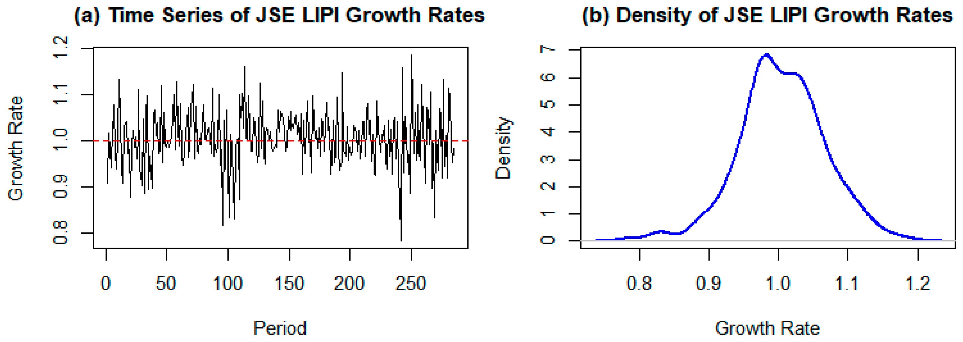
Monthly observations of the JSE Life Insurance Price Index (LIPI), expressed in ZAR, from January 2000 through October 2023 were used in this analysis. The data were sourced from Investing.com (https://www.investing.com/indices/ftse-jse-life-insurance-historical-data, accessed on 1 November 2024). Figure 1 presents the time series plots of JSE LIPI Growth Rates and JSE LIPI Growth Rate Losses density, and time series plots of the raw LIPI values $y_t$.

The growth rate series fluctuates around a baseline value of 1, with deviations above and below signalling periods of gains and losses. Losses are the ones below 1.00. The variability is clearly time-dependent, with clusters of heightened fluctuations appearing notably in the middle and later periods, indicative of volatility clustering, a common characteristic in financial time series. Examining the growth rate losses series highlights pronounced downside spikes and grouped extreme losses, pointing to heavy-tailed behaviour and underscoring the suitability of Extreme Value Theory (EVT) for capturing tail risk.

4.2. Preliminary Diagnostic Analysis

Before model estimation, several diagnostic tests were conducted to evaluate the statistical properties of the full sample of JSE LIPI growth rates, prior to focusing on extreme losses. Stationarity was examined using the Augmented Dickey–Fuller (ADF) test, where the null hypothesis indicates the presence of a unit root. Conditional heteroscedasticity was assessed using the ARCH-Lagrange multiplier test, and serial dependence was evaluated using the Ljung–Box Q-statistic. The results of these tests are reported in

Table 1. Statistical Diagnostic Tests for JSE LIPI growth rates.

Test	Test Statistic	Lag/df	p-Value
Augmented Dickey–Fuller (ADF)	−5.2821	6	0.0100
ARCH LM	8.4978	5	0.1309
Ljung–Box Q	3.0597	5	0.6908

.

The ADF test statistic of −5.2821 (p = 0.0100) leads to rejection of the null hypothesis of a unit root at the 5% significance level, confirming that the JSE LIPI growth rate series is stationary. The ARCH-LM test (8.4978, df = 5, p = 0.1309) indicates no significant evidence of conditional heteroscedasticity, while the Ljung–Box Q-statistic (3.0597, df = 5, p = 0.6908) suggests no strong serial correlation in the series at conventional significance levels. These results support the stationarity and weak serial dependence of the growth rate series, providing a suitable basis for applying the GEVD to model extreme losses. Nonetheless, mild residual dependence or volatility clustering cannot be entirely ruled out, which is common in financial return series, but the presented results still support the applicability of the GEVD and GPD.

4.3. Modelling Extreme Losses

4.3.1. BM Approach

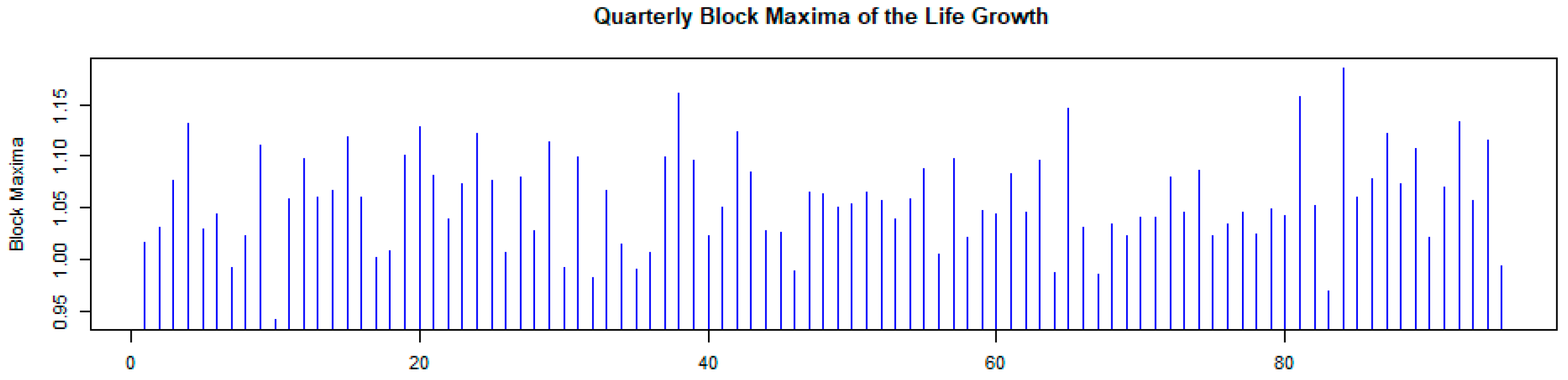
To analyse the most severe downward movements in the JSE LIPI, the BM method was applied to the monthly growth rate series. Quarterly blocks were chosen to capture economic periods with sufficient observations for robust estimation. This block size balances the need to capture significant extreme events while maintaining a manageable sample size per block. Each quarter, comprising three months, was treated as a separate, non-overlapping block, yielding 95 quarterly blocks. Within each block, the largest loss is defined as the highest positive value in the transformed loss series, and $L_t$ was selected to represent that quarter. The resulting series of monthly loss maxima forms the dataset used to fit the GEVD, which is well-suited for modelling extreme events in time series data.

Figure 2 presents the series of quarterly maximum losses (95 observations) derived from the JSE LIPI, highlighting the most significant adverse movements in each quarter.

Figure 2 displays the quarterly block maxima of the transformed LIPI growth rate losses. The plot reveals noticeable variability in the magnitude of extreme losses across quarters. Several pronounced spikes are observed, indicating periods of substantial adverse movements in the index. The clustering of large positive spikes reflects episodic extreme downturns, justifying the application of the GEVD for modelling tail risk.

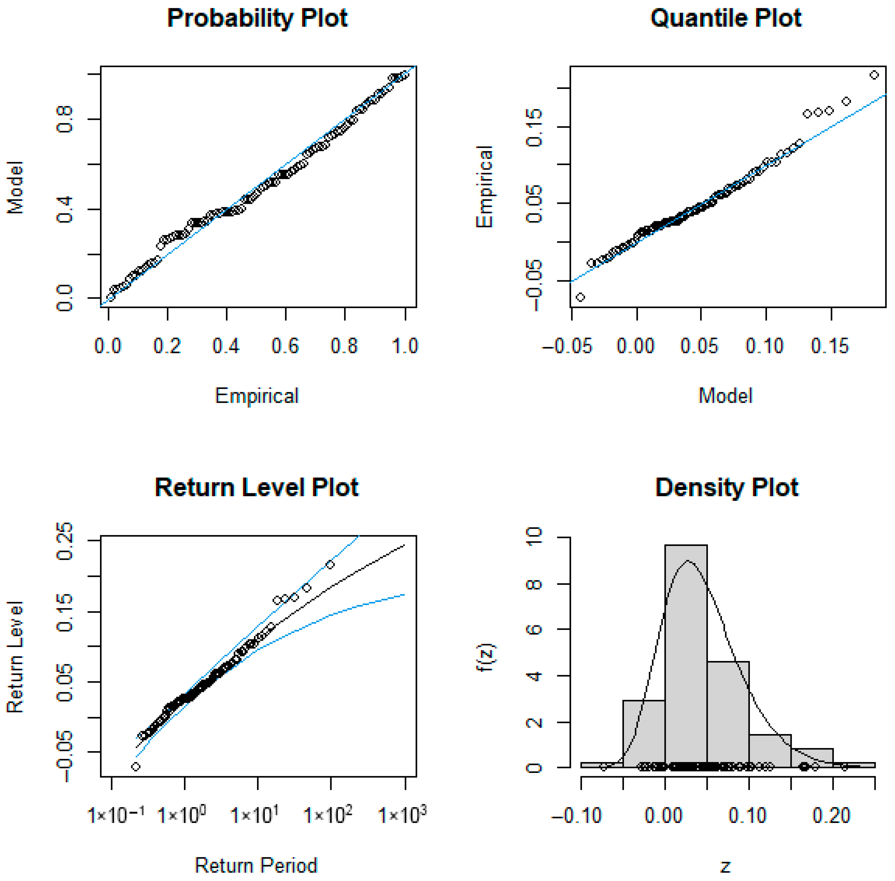
Figure 3 presents the diagnostic plots obtained from fitting the GEVD to the quarterly block maxima of the transformed loss series $L_t$. The model parameters were estimated using the MLE method. The quantile–quantile (QQ) and probability–probability (PP) plots assess the agreement between empirical and theoretical distributions, the density plot compares the fitted model to the observed block maxima, and the return level plot examines the model’s ability to estimate extreme loss magnitudes over longer return periods. These diagnostics provide a comprehensive assessment of model adequacy and support inference regarding rare but economically significant adverse movements.

The PP plot shows that the empirical probabilities closely follow the 45-degree reference line, indicating strong agreement between the observed data and the fitted GEVD across most of the range. The Q-Q plot demonstrates good alignment in the central region, with slight deviations in the upper tail. The mild upward departure of the largest observations suggests that the model slightly underestimates the most extreme losses, although the overall fit remains satisfactory. The Return Level plot indicates that empirical return levels closely track the fitted GEVD curve within the confidence bands, particularly for shorter return periods. Some divergence appears at higher return periods, reflecting increased uncertainty in extrapolating rare extreme events. The Density plot shows that the fitted GEVD density plot captures the general shape and dispersion of the block maxima distribution, with a moderately right-skewed tail, consistent with extreme-loss behaviour. The diagnostic plots suggest that the GEVD provides an adequate representation of extreme losses in the LIPI growth rates, with minor tail deviations typical in finite samples.

4.3.2. Peaks-over-Threshold (POT) (GPD) Approach

To complement the block maxima approach, the Peaks-Over-Threshold (POT) method was applied to the JSE LIPI growth rate losses. Unlike the block maxima method, POT uses all observations exceeding a high threshold, allowing more efficient use of extreme events.

Threshold Selection

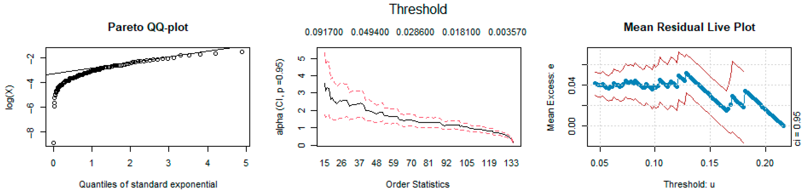
The threshold selection for the POT method was guided by three diagnostic tools: the Pareto QQ plot, Hill plot, and Mean Residual Life plot. These three methods were used to select a suitably high threshold to fit the GPD to the values in excess of the threshold. A threshold $u$ was chosen at the 95th percentile of the loss distribution ($u=0.05$) based on the mean residual life plot and threshold stability plot (Figure 4). This ensures that only the most extreme observations are modelled while maintaining a sufficient sample size for reliable parameter estimation.

The Pareto QQ plot indicated approximate linearity in the upper tail, suggesting a threshold of around 0.04. The Hill plot showed a stable region between order statistics 75 and 88, supporting a threshold in the range of 0.04–0.05. The Mean Residual Life plot displayed a linear upward trend beginning near 0.04, with instability observed at higher thresholds. Based on this combined evidence, a threshold of $u=0.04$ was selected for the GPD modelling of extreme losses.

4.4. Parameter Estimates (GEVD vs. GPD)

To model the extreme fluctuations in the life insurance growth rates $x_t$, the GEVD and GPD were fitted using MLE.

Table 2. Parameter Estimates Using the MLE for GEVD and GPD.

Model	Shape Parameter	SE (Shape)	Scale Parameter	SE (Scale)	Location
GEVD	−0.0776	0.0046	0.0412	0.0031	0.0244
GPD	0.0433	0.0147	0.0400	0.0086	–

summarises the estimated parameters of the GEVD and GPD models, including the shape, scale, and location parameters, along with their standard errors.

The GEVD model yields a negative shape parameter, indicating a bounded upper tail consistent with a Weibull-type distribution. In contrast, the GPD model produces a positive shape parameter, suggesting a heavy-tailed distribution. This difference implies that while the GEVD assumes a finite upper limit to extreme losses, the GPD allows for more severe and unbounded tail behaviour. The scale parameters for both models are relatively similar, indicating comparable dispersion in extreme losses, although the GPD exhibits slightly higher estimation uncertainty.

4.5. Return Level Estimates for Life Insurance Price Index Growth Rate Losses

Table 3. GEVD and GPD Return Level Estimates for LIPI Indices Growth Rate Losses.

Return Period	GEVD (Point)	GPD (Point)	GEVD CI	GPD CI
2 years	0.040	0.249	(0.029–0.051)	(0.137–0.361)
5 years	0.085	0.276	(0.071–0.101)	(0.125–0.427)
20 years	0.138	0.315	(0.116–0.168)	(0.095–0.534)
50 years	0.170	0.338	(0.141–0.215)	(0.069–0.608)
100 years	0.192	0.355	(0.157–0.252)	(0.046–0.665)

presents the return level estimates for extreme monthly losses within a quarter in the JSE LIPI growth rates, obtained from both the GEVD and the GPD. Each return level represents the magnitude of loss expected to be exceeded, on average, once over a specified return period.

The estimates are reported together with their corresponding 95% confidence intervals, providing a measure of uncertainty associated with extreme loss projections. These results facilitate a direct comparison of return levels derived from the BM and POT approaches.

The GEVD-based return-level estimates in Table 3 quantify the magnitude of extreme monthly losses within a quarter expected over different return periods. A 2-year return level of 0.040 (95% credible interval: 0.029–0.051) indicates that, on average, a loss of this magnitude or greater is expected once every 2 years. Similarly, the 100-year return level of 0.192 (95% CI: 0.157–0.252) represents a very rare but severe loss, expected to be exceeded only once in a century. The widening of the credible intervals for longer return periods reflects increased uncertainty in estimating rarer events, a characteristic feature of extreme-value modelling. These results highlight the tail risk inherent in the JSE LIPI and provide a probabilistic framework for assessing potential extreme monthly losses within a quarter, which is valuable for risk management and regulatory capital planning.

For the GPD model, a 2-year return level of approximately 0.249 (95% CI: 0.137–0.361) represents a relatively frequent extreme loss, while the 100-year return level of 0.355 (95% CI: 0.046–0.665) reflects a rare but severe event. As expected, return levels increase with the return period, indicating greater loss severity for less frequent occurrences. The confidence intervals widen considerably for longer return periods, reflecting increased uncertainty when extrapolating extreme quantiles beyond the observed data range. These results highlight the significant tail risk in life insurance growth rate losses and demonstrate the suitability of the GPD model for capturing extreme events.

4.6. GEVD and GPD-Based VaR and tVaR Estimates for LIPI Growth Rate Losses

Table 4. GEVD and GPD Model–Based VaR and tVaR Estimates.

Confidence Level	GEVD Parametric VaR	GEVD Empirical VaR	GEVD Parametric tVaR	GEVD Empirical tVaR	GPD Parametric VaR	GPD Empirical VaR	GPD Parametric tVaR	GPD Empirical tVaR
90%	0.1095	0.1034	0.1425	0.1475	0.0679	0.0674	0.1104	0.1062
95%	0.1338	0.1382	0.1645	0.1796	0.0962	0.0963	0.1402	0.1332
97.5%	0.1562	0.1682	0.1852	0.1888	0.1233	0.1199	0.1689	0.1583
99%	0.1839	0.1832	0.2107	0.2162	0.1574	0.1672	0.2049	0.1888

presents the parametric and empirical estimates of VaR and tVaR, or ES for quarterly JSE LIPI growth-rate losses, based on both the GEVD and GPD models. VaR represents the loss level unlikely to be exceeded at a given confidence level, while tVaR captures the average severity of losses beyond VaR. Comparing the GEVD and GPD results provides insight into the relative conservativeness and reliability of the two extreme-value approaches for assessing tail risk and informing risk management and capital planning in the life insurance sector.

At the 90% confidence level, the GEVD-based parametric VaR of 0.1095 indicates that a loss of this magnitude or greater is expected only 10% of the time, with the corresponding parametric tVaR of 0.1425 representing the average extreme loss beyond this threshold. As confidence levels increase to 99%, both VaR and tVaR rise, reflecting rarer but more severe losses. The empirical GEVD estimates are slightly higher, suggesting that observed losses are marginally more severe than the model predicts.

For the GPD model, the 90% parametric VaR of 0.0679 and tVaR of 0.1104 similarly capture the risk of extreme losses, with estimates increasing with higher confidence levels. Compared to GEVD, GPD VaR values are generally lower, while tVaR values are comparable, indicating that GPD is slightly more conservative for tail risk at higher confidence levels. Both models provide a probabilistic framework for assessing extreme losses, with GEVD showing slightly more robust coverage across the tail.

4.7. Kupiec Backtest Results

To assess the reliability of extreme-loss estimates, Kupiec Unconditional Coverage (UC) Tests were conducted for both GEVD- and GPD-based VaR estimates. This test evaluates whether the observed frequency of VaR exceedances matches the expected frequency implied by the model. A p-value greater than 0.05 indicates that the null hypothesis of correct coverage cannot be rejected, meaning the model’s predicted risk thresholds are statistically consistent with the observed losses. Conversely, a p-value below 0.05 suggests the model underestimates or overestimates extreme losses.

Table 5. Kupiec Backtest Results Based VaR Estimates.

Confidence Level	GEVD Kupiec p-Value	GEVD Adequacy	GPD Kupiec p-Value	GPD Adequacy
90%	0.8632	Adequate	0.0000	Inadequate
95%	0.9071	Adequate	0.0079	Inadequate
97.5%	0.1319	Adequate	0.0122	Inadequate
99%	0.9592	Adequate	0.4423	Adequate

compares the Kupiec backtest results for GEVD- and GPD-based VaR estimates. The GEVD model shows p-values well above the 5% threshold across all confidence levels, indicating reliable coverage of both moderate and extreme losses. In contrast, the GPD model passes the test only at the 99% level, suggesting it underestimates risk at lower confidence levels. The GEVD-based VaR provides more robust and consistent coverage, while the GPD is more conservative for tail extremes.

5. Discussion

The GEVD and GPD modelling results for LIPI growth-rate losses provide important insights into extreme loss behaviour in the South African insurance and financial markets. The Kupiec backtest results indicate that GEVD-based Value-at-Risk (VaR) estimates consistently capture both moderate and extreme losses across all confidence levels, while the GPD-based VaR underestimates risk at lower confidence levels. This finding aligns with prior research, which shows that block maxima approaches such as GEVD often provide more reliable tail risk estimates than threshold exceedance models like GPD when sample sizes are finite [24,27].

The upward trend in return levels over longer horizons reflects the fat-tailed nature of loss distributions, a characteristic widely documented in the extreme-value theory literature [20,28]. The wider confidence intervals observed at the 50- and 100-year horizons demonstrate the inherent uncertainty in estimating rare events, emphasising that extreme loss estimates, while informative, remain subject to sampling limitations [19]. These findings suggest that while GEVD provides statistically consistent risk thresholds, caution must be exercised when interpreting long-horizon estimates due to the increased variability associated with rare events.

The comparison between GEVD and GPD models further underscores the importance of model selection in extreme-value analysis. The GPD model’s failure to adequately capture tail risk at lower confidence levels indicates that threshold exceedance methods may be more conservative or less robust depending on the data structure and threshold choice. This is consistent with findings from previous studies demonstrating that GEVD-based approaches generally offer more stable coverage in finite samples [29,30]. The results highlight the relevance of EVT-based measures for risk management, particularly for insurers aiming to quantify tail risk and optimise capital allocation.

Although systemic shocks, including economic disruptions, can exacerbate losses, this study does not directly measure such events. Therefore, any implications regarding sensitivity to shocks or events such as pandemics should be interpreted cautiously, as they are not empirically tested within the scope of this research. Nonetheless, the findings reinforce the utility of EVT-based measures for capturing potential extreme outcomes, supporting risk management strategies that consider events beyond historically observed scenarios.

6. Conclusions

This study has demonstrated that GEVD-based VaR estimates provide reliable coverage for extreme losses in LIPI growth rates, outperforming GPD-based estimates at most confidence levels. The application of extreme-value theory to the South African insurance market, combined with Kupiec backtesting, provides evidence of methodological rigour and supports the use of EVT-based metrics for tail risk assessment. The research contributes to the literature by highlighting the robustness of block maxima models in estimating extreme losses and by demonstrating the limitations of threshold exceedance models in finite samples.

The results suggest that insurers can enhance capital planning and enterprise risk management by incorporating GEVD-derived tail risk measures. Scenario analysis that extends beyond historical experience is particularly valuable for assessing potential extreme events and ensuring the adequacy of solvency buffers. Methodologically, the study underscores the importance of model selection and careful consideration of statistical adequacy in EVT applications.

Several limitations should be noted. The analysis relies exclusively on historical LIPI growth-rate data and does not incorporate macroeconomic covariates or direct measures of systemic shocks. The estimation of long-horizon return levels is inherently uncertain due to the finite sample size, a limitation widely acknowledged in EVT studies. The findings are specific to the South African insurance sector and may not generalise to other markets without additional validation.

Future research could extend this analysis by investigating relationships between extreme LIPI losses and broader financial market conditions, including capital market fluctuations. Incorporating macroeconomic variables or stress scenarios would allow quantification of systemic shocks’ impacts on extreme losses. Additionally, multivariate EVT approaches could be explored to assess joint tail risks across different insurance lines or financial instruments, thereby enhancing understanding of risk propagation in emerging financial markets.