Enhancing Data Quality with a Novel Neural Parameter Diffusion Approach

Abstract

This study presents a novel neural parameter diffusion approach (FWA-PDiff) designed to enhance data quality. To address the limitations of conventional diffusion models—such as inefficient sampling and insufficient feature sensitivity, which may compromise output fidelity—this study introduces four key innovations. First, the proposed model introduces an adaptive recalibration of the sampling frequency in the Fourier domain to optimize feature extraction for image data. Second, a dual-channel autoencoder architecture is employed, featuring a multi-scale, fine-grained encoder (MFE) that enables the simultaneous capture of features at multiple resolutions. Third, a wavelet-attention mechanism (WA) is incorporated into the decoder to highlight subtle high-frequency details. Fourth, the proposed model introduces a hybrid loss function that combines Mean Squared Error (MSE) and Kullback–Leibler (KL) divergence to improve data reconstruction. Collectively, these improvements enable the generation of high-fidelity parameters, thereby contributing to enhanced data quality. Extensive experiments conducted on benchmark datasets—including MNIST, CIFAR-10, CIFAR-100, and STL-10—demonstrate the effectiveness of the proposed approach, which consistently achieves superior performance in improving data quality.

1. Introduction

Diffusion models, rooted in non-equilibrium thermodynamics [1], have emerged as a powerful class of generative models capable of synthesizing high-quality data through progressive denoising. The seminal work in [2] formalized the diffusion process for image generation and established a rigorous mathematical foundation for subsequent research. Building on this framework, ref. [3] introduced a hybrid objective that combines the variational lower bound (VLB) with denoising diffusion probabilistic models (DDPM), together with reparameterized variance estimation. This improvement significantly enhanced log-likelihood performance and gradient stability. Another important breakthrough concerned sampling efficiency. The number of inference steps was reduced from approximately 1000 to around 100 without sacrificing output quality, thereby enabling diffusion models to be applied in more computationally demanding scenarios. Subsequently, the work in [4] further improved generative performance by incorporating classifier guidance with a second-order Taylor expansion. This approach produced the first diffusion model that surpassed Generative Adversarial Networks (GANs) in sample fidelity. These advances inspired a series of conditional generation techniques. Among them, GLIDE [5] became one of the dominant approaches prior to the emergence of latent diffusion models (LDMs). Later, ref. [6] innovatively deployed diffusion processes in the latent space by adopting an encoder–decoder architecture similar to that used in variational autoencoders. This framework also systematically integrated cross-attention mechanisms, which have since become a standard component in many multimodal diffusion systems. More recently, ref. [7] achieved state-of-the-art performance in image, video, and text generation by replacing the traditional U-Net architecture with a Transformer-based model. Most relevant to our work, P-diff [8] pioneered the application of denoising diffusion models to neural network parameter generation. Their study demonstrated the feasibility of structured parameter synthesis and opened a new paradigm for model-based data enhancement.

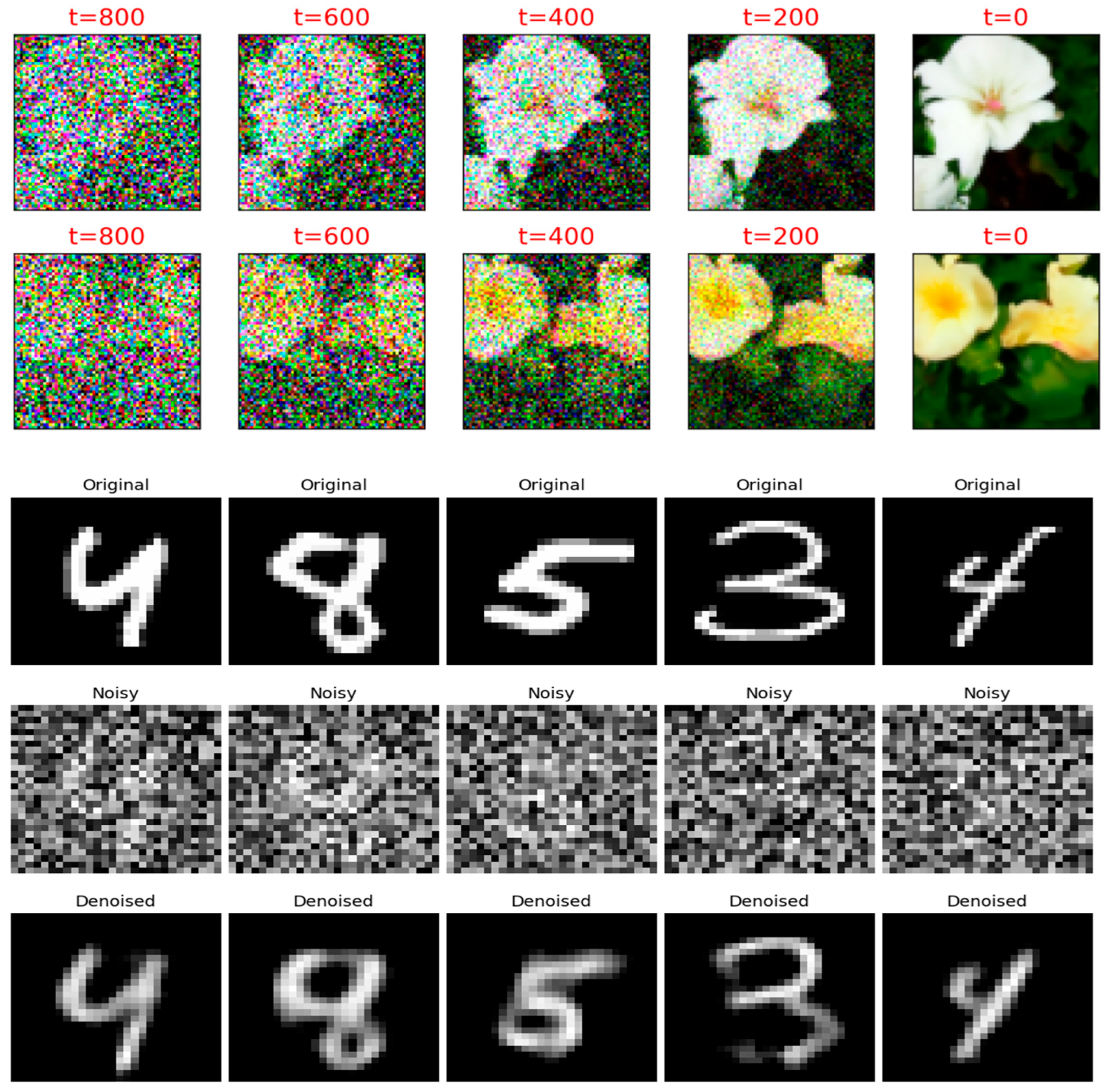
Despite these advances, the training efficiency and output quality of diffusion models remain strongly influenced by the choice of time-step sampling strategy. The linear sampling scheme used in P-diff adopts uniform intervals across the diffusion trajectory. However, this strategy does not adapt to the stage-dependent sampling requirements of the diffusion process. In particular, during the early diffusion stages, the data structure is largely preserved, and excessive sampling introduces unnecessary computational overhead and inefficient resource utilization. To address this issue, IDDPM [9] proposed a cosine-based time-step sampling strategy. This method distributes sampling points non-uniformly according to the noise intensity, thereby allocating model attention and computational resources more effectively. Furthermore, by leveraging the frequency decomposition capability of the Fourier transform, the sampling schedule can be further refined in the spectral domain. Such refinement can better align with multi-scale and fine-grained encoder designs [10]. Meanwhile, high-resolution images inherently contain rich multi-scale information. However, the autoencoder used in P-diff is unable to fully capture these hierarchical features. This limitation restricts the recovery of fine-grained visual details and ultimately constrains the quality of both the generated parameters and the resulting data. The parameter diffusion approach for image generation is illustrated in Figure 1. As shown in the figure, the proposed model effectively suppresses noise while preserving structural details, demonstrating its qualitative advantages.

To overcome these limitations, this paper proposes FWA-PDiff, which is enhanced with four key innovations as described in the abstract. The goal of the proposed framework is to improve data quality through high-fidelity parameter generation. The main contributions of this work are summarized as follows.

The overall pipeline operates as follows. First, a subset of model parameters, pre-trained using stochastic gradient descent (SGD), is encoded by the proposed dual-channel autoencoder under the Fourier-optimized time-step schedule. Next, the extracted multi-scale features are fused into a unified latent representation. This representation is then reconstructed through a diffusion process initialized from random noise. Finally, the decoder generates improved model parameters, which in turn lead to enhanced data quality in downstream tasks.

The FWA-PDiff has four principal benefits:

• Optimize the sampling strategy of P-diff to better align with the spectral properties of the training dynamics.
• Strengthen fine-grained and multi-scale feature extraction through architectural and attentional refinements.
• Yield neural network parameters that achieve superior accuracy, average precision, and median performance, thereby tangibly enhancing the quality of generated data.
• Introduce the KL divergence function on top of the MSE function, forming a mixed error function of MSE-KL divergence, which smoothly focuses on extreme noise values.

2. Methods

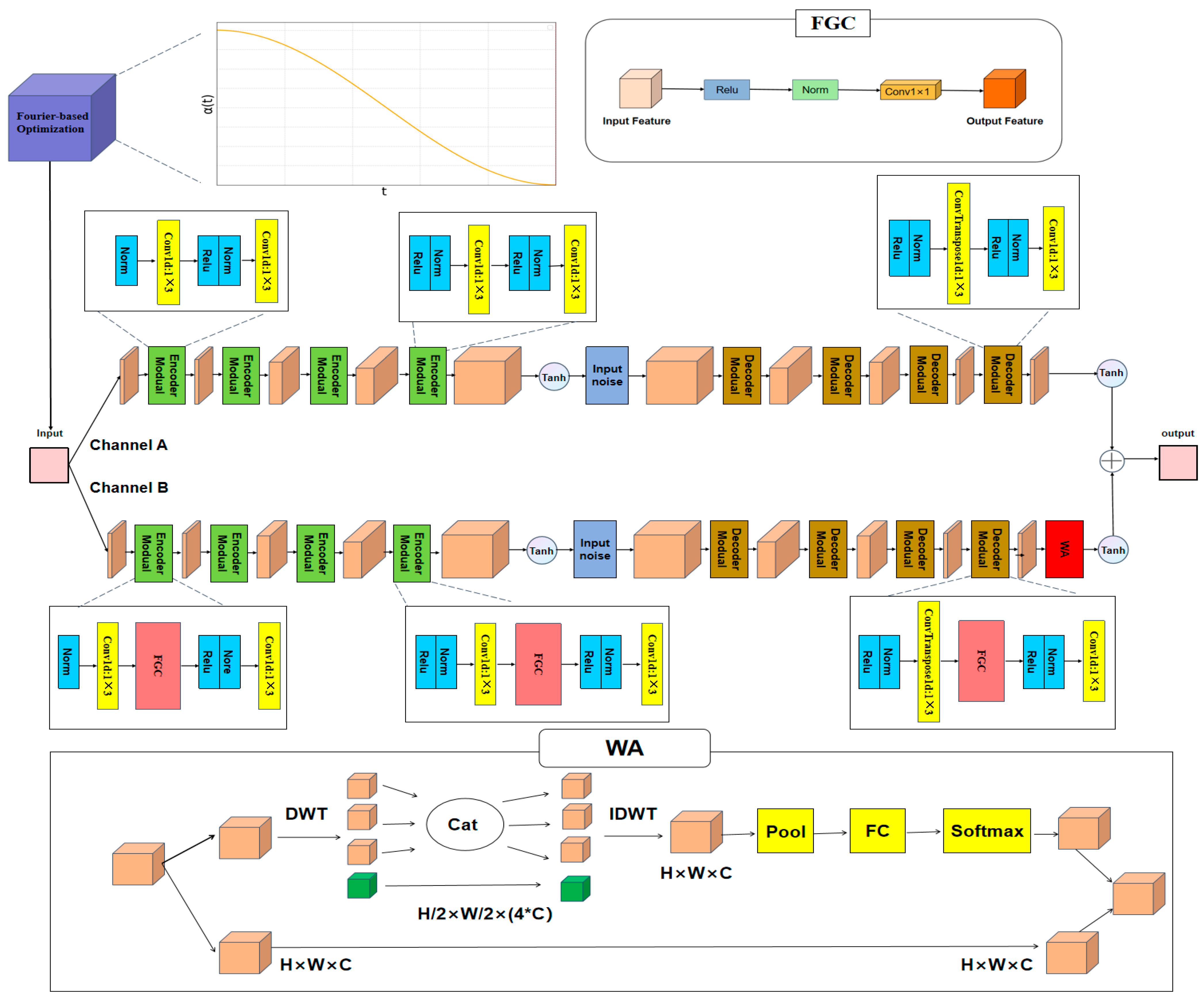
Firstly, the optimal sampling frequency formula is refined using the Fourier transform. Then, an MFE trains the input image based on the optimized sampling frequency. The input image undergoes feature extraction through both convolutional channel A and channel B. After passing through the first half of the Encoder Module, the feature information is processed for noise reduction before being fed into the Decoder Module. The feature information extracted from the final two channels is cut and concatenated to form the final output feature. The overall network structure of the neural network parameter diffusion model based on multi-scale Fourier transform is shown in Figure 2.

2.1. FFG Method

The core value of Fourier optimization in this context lies in explicitly modeling the periodic characteristics of noise through frequency decomposition, enabling precise regulation of information degradation rates across different frequency components. Specifically, this mathematical framework effectively suppresses high-frequency noise interference while preserving low-frequency structural information, thereby enhancing the stability of the sampling process and the quality of final results. The cosine periodic sampling inherent in Fourier analysis employs high-frequency sampling during the initial phase, facilitating more efficient learning of image details on images not yet extensively corrupted by noise; in the later sampling stages, for images already degraded by noise, lower-frequency sampling is utilized to learn image features, thereby improving overall sampling efficiency and reducing computational resource consumption.

Based on the periodicity of cosine sampling time steps proposed in reference IDDPM, this study introduces Fourier transform to optimize the sampling process in the diffusion model P-diff. By utilizing the property of Fourier series, periodic signals can be decomposed into sine and cosine functions of different frequencies. The time step of periodic sampling can thus be represented as a combination of multiple frequency components. This method aims to effectively reduce the number of steps required for traditional linear sampling, while enhancing the model’s adaptability to convolutional structures of different sizes and shapes and improving the flexibility of feature extraction. In terms of model structure design, Fourier transform is applied to the forward sampling of diffusion models through the following steps: Firstly, a sampling time step sequence suitable for different frequency components is generated based on the Fourier series principle. Then, the model performs sampling and trains an autoencoder based on this sequence. This method reduces the number of forward passes by an order of magnitude without compromising generation quality, significantly improving sampling efficiency and inference speed. Additionally, the sampling frequency optimization strategy based on Fourier series can adaptively adjust the sampling scheme according to the characteristics of different datasets, thereby significantly improving parameter accuracy in neural network parameter generation tasks. The experimental results show that this method exhibits excellent robustness and generalization ability in multiple tasks. The Fourier series fitting cosine time step formula is derived as follows:

The cosine sampling time step formula, proposed in [8], is defined as follows:

$${\alpha }_{\mathrm{t}}={\displaystyle \frac{{\cos }^2(\frac{\mathrm{t}+\mathrm{s}}{\mathrm{T}+2\mathrm{s}}\cdot \frac{\pi }{2})}{{\cos }^2(\frac{s}{T+2s}\cdot \frac{\pi }{2})}}$$

(1)

In Equation (1), t denotes the time step, T represents the total number of time steps, and s indicates a small offset parameter. According to established literature, s is typically configured to 0.008. The adoption of cosine sampling time steps addresses the critical issue of excessive noise accumulation in later stages—a limitation inherent to linear noise scheduling that degrades sampling quality. In contrast, cosine sampling facilitates a smoother degradation process of information throughout the diffusion sequence.

• To simplify Equation (1), this study employs trigonometric identity transformation. The relevant trigonometric identity is presented below:

$${\cos }^{2}x={\displaystyle \frac{1+\cos (2x)}{2}}$$

(2)

The simplification process yields the following result:

$${\alpha }_{\mathrm{t}}={\displaystyle \frac{1+\cos (\frac{\pi (t+s)}{T+2s})}{1+\cos (\frac{\pi s}{T+2s})}}$$

(3)

Given the original framework parameters T = 1000 and s = 0.008, the denominator can be treated as a constant C, enabling further simplification:

$${\alpha }_{\mathrm{t}}={\displaystyle \frac{1}{C}}\left[1+\cos ({\displaystyle \frac{\pi (t+s)}{T+2s}})\right]$$

(4)

2.

Fourier Series Optimization Rationale: Fourier series decomposition enhances the cosine time-step formula by explicitly modeling periodic noise patterns, allowing more precise control over information degradation rates across different frequency components. This mathematical framework mitigates high-frequency noise artifacts while preserving low-frequency structural information, thereby improving sampling stability. To transform the cosine function in Equation (4) using Fourier series, this study first defines the function periodicity:

$$T_0={\displaystyle \frac{2\pi }{\omega }}, \omega ={\displaystyle \frac{\pi }{T+2s}}$$

(5)

$$T_0=2(T+2\mathrm{s})$$

(6)

Subsequently, this study calculates the Fourier coefficients through the following procedure:

$${\mathrm{a}}_0={\displaystyle \frac{1}{2(T+2s)}}{\displaystyle {\int }_0^{2(T+2S)}\cos (\frac{\pi (t+s)}{T+2s}})dt$$

(7)

Let

$$\theta ={\displaystyle \frac{\pi }{T+2\mathrm{s}}}t+{\displaystyle \frac{\pi s}{T+2s}}$$

then

$${\displaystyle \frac{d\theta }{dt}}={\displaystyle \frac{\pi }{T+2s}}, d\theta ={\displaystyle \frac{T+2s}{\pi }}dt$$

(8)

Integral bounds are defined as follows:

$${\theta }_1={\displaystyle \frac{\pi s}{T+2s}}$$

(9)

$${\theta }_2-{\theta }_1=2\pi$$

(10)

$${\mathrm{a}}_0={\displaystyle \frac{1}{2(T+2s)}}{\displaystyle {\int }_{{\theta }_1=\frac{\pi \mathrm{s}}{T+2s}}^{{\theta }_2=\frac{\pi (2T+5\mathrm{s})}{T+2s}}\cos \theta •\frac{T+2s}{\pi }}d\theta$$

(11)

$$={\displaystyle \frac{1}{2\pi }}{\displaystyle {\int }_{{\theta }_1}^{{\theta }_2}\cos \theta d\theta }$$

(12)

$$={\displaystyle \frac{1}{2\pi }}{\displaystyle {\int }_{{\theta }_1}^{{\theta }_{1+2\pi }}\cos \theta d\theta =0}$$

(13)

To compute the Fourier coefficients ${\mathrm{a}}_n$:

$${\mathrm{a}}_n={\displaystyle \frac{2}{2(T+2s)}}{\displaystyle {\int }_0^{2(T+2s)}\cos (\frac{\pi (t+s)}{T+2s}})\cos ({\displaystyle \frac{n\pi t}{T+2s}})dt$$

(14)

Let L = T + 2s; substituting this into Equation (14) yields:

$${\mathrm{a}}_{\mathrm{n}}={\displaystyle \frac{1}{L}}{\displaystyle {\int }_0^{2L}\cos (\frac{\pi (t+s)}{L})}\cos ({\displaystyle \frac{n\pi t}{L}})dt$$

(15)

Applying the trigonometric product-to-sum identity:

$$\cos A\cos B={\displaystyle \frac{1}{2}}\left[\cos (A+B\right.)+\left.\cos (A-B)\right]$$

(16)

Let

$$A={\displaystyle \frac{\pi (t+s)}{L}}={\displaystyle \frac{\pi t+\pi s}{L}}, B={\displaystyle \frac{\mathrm{n}\pi t}{\mathrm{L}}}$$

(17)

Then:

$$A+B={\displaystyle \frac{\pi \mathrm{t}}{L}}(1+n)+{\displaystyle \frac{\pi s}{L}}, A-B={\displaystyle \frac{\pi \mathrm{t}}{L}}(1-n)+{\displaystyle \frac{\pi \mathrm{s}}{\mathrm{L}}}$$

(18)

$${\mathrm{a}}_{\mathrm{n}}={\displaystyle \frac{1}{L}}{\displaystyle {\int }_0^{2L}\cos (\frac{\pi (t+s)}{L})}\cos ({\displaystyle \frac{n\pi t}{L}})dt$$

(19)

$${\mathrm{a}}_{\mathrm{n}}={\displaystyle \frac{1}{L}}({\displaystyle {\int }_0^{2L}\cos (\frac{\pi (1+n)}{L}t+\frac{\pi s}{L})}dt+{\displaystyle {\int }_0^{2L}\cos (\frac{\pi (1-n)}{L}t+\frac{\pi s}{L})}dt)$$

(20)

Let

$$k_1={\displaystyle \frac{\pi (1+n)}{L}}, \varphi ={\displaystyle \frac{\pi s}{L}}$$

(21)

then:

$${\mathrm{a}}_n={\displaystyle \frac{1}{L}}({\left[{\displaystyle \frac{\sin (k_{1}t+\varphi )}{k_1}}\right]}_0^{2L}+{\displaystyle {\int }_0^{2L}\cos (\frac{\pi (1-n)}{L}t+\frac{\pi s}{L})}dt)$$

(22)

$${\mathrm{a}}_n={\displaystyle \frac{1}{L}}(\left[{\displaystyle \frac{\sin (k_1\cdot 2L+\varphi )-\sin (\varphi )}{k1}}\right]+{\displaystyle {\int }_0^{2L}\cos (\frac{\pi (1-n)}{L}t+\frac{\pi s}{L})}dt)$$

(23)

$${\mathrm{k}}_1\cdot 2L=2\pi (1+n)$$

(24)

$${\mathrm{a}}_n={\displaystyle \frac{1}{L}}{\displaystyle {\int }_0^{2L}\cos (\frac{\pi (1-n)}{L}t+\frac{\pi s}{L})}dt$$

(25)

Similarly, substituting the following variables:

$$k_1={\displaystyle \frac{\pi (1-n)}{L}}, \varphi ={\displaystyle \frac{\pi s}{L}}$$

(26)

For n = 1, the resulting expression is

$${\mathrm{a}}_1=\cos ({\displaystyle \frac{\pi s}{T+2\mathrm{s}}})$$

(27)

when n ≠ 1 and n > 0, ${\mathrm{a}}_1=0$.

Similarly, the Fourier coefficients ${\mathrm{b}}_n$ are computed using the product-to-sum identity and substitution method:

$${\mathrm{b}}_n={\displaystyle \frac{2}{2(T+2s)}}{\displaystyle {\int }_0^{2(T+2s)}\cos (\frac{\pi (t+\mathrm{s})}{T+2s}})\sin ({\displaystyle \frac{n\pi t}{T+2s}})dt$$

(28)

For n = 1, the calculation yields

$$b_1=\sin ({\displaystyle \frac{\pi s}{T+2\mathrm{s}}})$$

(29)

For n = 1, the result is $b_n=0$.

3.

The Fourier series ${\mathrm{a}}_0$, ${\mathrm{a}}_n$, ${\mathrm{b}}_n$ transformation expression is formulated as:

$$\cos ({\displaystyle \frac{\pi (t+s)}{T+2s}})={\mathrm{a}}_0+a_1\cos ({\displaystyle \frac{\pi t}{T+2s}})-b_1\sin ({\displaystyle \frac{\pi t}{T+2s}})$$

(30)

With T = 1000 and s = 0.008,

$$a_1=\cos ({\displaystyle \frac{\pi s}{T+2s}})\approx 1, {\mathrm{b}}_1=\sin ({\displaystyle \frac{\pi s}{T+2s}})\approx 0$$

(31)

$$\cos ({\displaystyle \frac{\pi (t+s)}{T+2s}})\approx \cos ({\displaystyle \frac{\pi s}{T+2s}})$$

(32)

Substituting Equation (33) into Equation (4) yields the final Fourier series cosine time-step formula:

$${\alpha }_{\mathrm{t}}={\displaystyle \frac{1}{C}}\left[1+\cos ({\displaystyle \frac{\pi t}{T+2s}})\right]$$

(33)

Equation (34) is a simplified representation of the sampling time step obtained through Fourier series transformation of Equation (1), incorporating the Fourier frequency domain characteristics. Compared with linear time steps, this design concentrates computational resources on critical stages that significantly impact generation quality, thereby effectively reducing redundant training (e.g., avoiding excessive optimization of subsequent time steps) and accelerating model convergence. Under identical sampling step conditions, this method generates neural network parameters with higher-quality details, and the training process demonstrates improved stability—particularly during the early training stages. Additionally, this method exhibits stronger adaptability to high-resolution data and is better suited for extracting subtle image features.

2.2. MFE Model

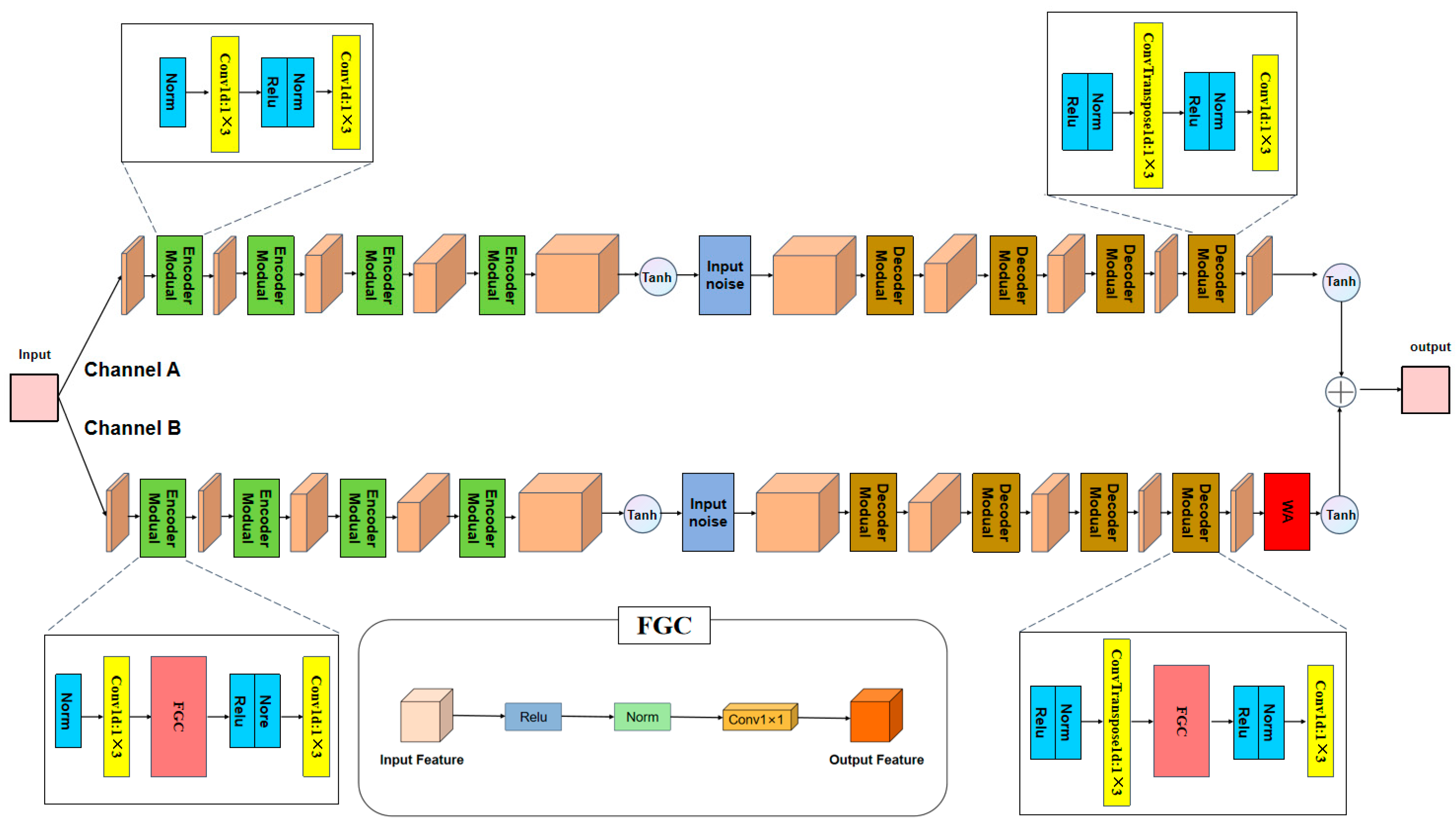
Traditional denoising autoencoders, such as the architecture proposed in P-diff, exhibit several critical limitations when processing large-scale and complex datasets. First, coarse-grained convolution operations result in insufficient perception of subtle features, which leads to the loss of fine-grained structural information. Second, the single-channel architecture restricts the feature hierarchy and fails to capture multi-scale contextual information, thereby reducing the accuracy of the generated neural network parameters. To address these issues, this study proposes an MFE architecture with two main design motivations. First, inspired by the dual-path network structures proposed in [11], a dual-channel convolutional architecture is adopted by introducing an additional channel (Channel B) to replace the original single-channel structure. This parallel feature extraction mechanism enhances the model’s information capture capability by fusing complementary features from the two channels, thereby improving the overall feature representation capacity. Second, fine-grained convolution (FGC) units [12] are embedded into the four encoder and decoder modules of Channel B to strengthen local structure characterization and subtle feature extraction. Through this differentiated feature processing mechanism, the accuracy and stability of neural network parameter generation are significantly improved. Specifically, the input image is simultaneously fed into Channel A and Channel B for parallel feature extraction and processing.

• Channel A processing flow:
  • The input passes through four identical encoder modules. Each module consists of two consecutive ReLU + Norm + Conv 1 × 3.
  • The Tanh function is then applied, followed by noise injection.
  • After passing through the four identical encoder modules, the data flows through four identical decoder modules. Each decoder module also consists of two consecutive ReLU + Norm + Conv 1 × 3 operations.
• Channel B processing flow:
  • The input passes through four identical encoder modules. Each module contains two ReLU + Norm + Conv 1 × 3.
  • The Tanh function is applied, followed by noise injection.
  • After passing through the four identical encoder modules, the data flows through four identical decoder modules. Each decoder module also contains two ReLU + Norm + Conv 1 × 3
  • The WA module is applied.

Finally, the image features extracted from the two channels at different scales are fused [13].

Design of the MFE: Traditional single-channel autoencoders suffer from two critical limitations in feature extraction. First, the sequential processing mechanism results in insufficient feature diversity, which leads to unstable representations of complex patterns. Second, such architectures cannot effectively capture multi-scale contextual information, which may cause the loss of subtle structural details. To address these issues, this study adopts a dual-channel parallel architecture for simultaneous feature extraction. In this architecture, Channel A maintains the original encoder–decoder structure in order to preserve the baseline feature extraction capability. In contrast, Channel B introduces differentiated processing to enhance feature richness and stability. Specifically, Channel B incorporates FGC modules into its Encoder/Decoder Modules. These modules significantly improve the model’s ability to capture subtle features by utilizing localized receptive fields and more refined feature extraction operations. The overall structure of the proposed MFE is illustrated in Figure 3.

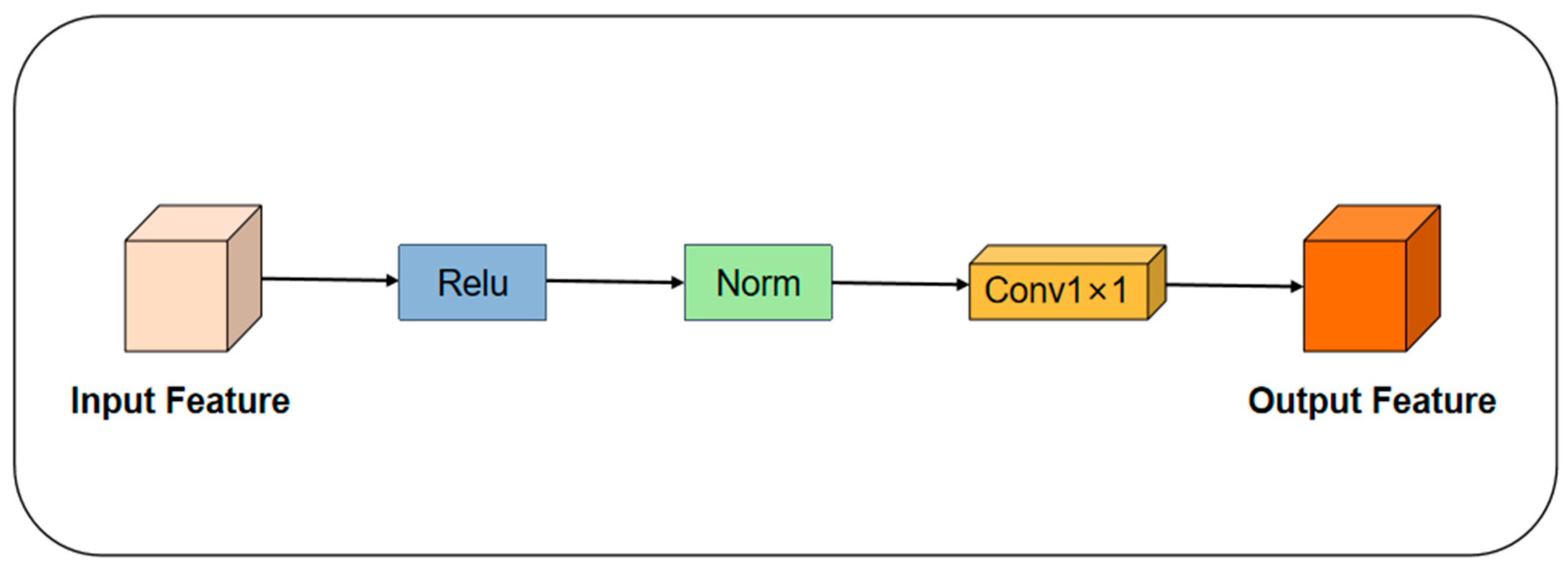
The FGC Structure: A critical challenge in diffusion-based parameter generation is the loss of semantic information during feature extraction by the autoencoder. This issue mainly arises from two limitations. First, coarse-grained convolution operations often fail to capture micro-level structural details. Second, single-scale feature processing cannot effectively model cross-dimensional dependencies, which leads to low precision in the generated parameters. To address these limitations, this study introduces a FGC feature enhancement module [10]. The proposed module improves feature representation through two complementary mechanisms. First, subtle feature capture is achieved by employing a 1 × 1 convolutional kernel combined with a sequential ReLU–Normalization processing pipeline. This design enables the FGC module to extract fine-grained features that are typically overlooked by conventional large-kernel convolution operations. Second, multi-scale feature enrichment is performed through the use of 1 × 1 convolutions across multiple scales. This mechanism allows the module to aggregate contextual information from different feature dimensions, thereby improving feature diversity and representation capability. Through these two improvements, the FGC module significantly enhances the semantic richness of the extracted features and effectively alleviates the precision bottleneck in neural network parameter generation. The overall structure of the FGC module is illustrated in Figure 4.

2.3. WA Model

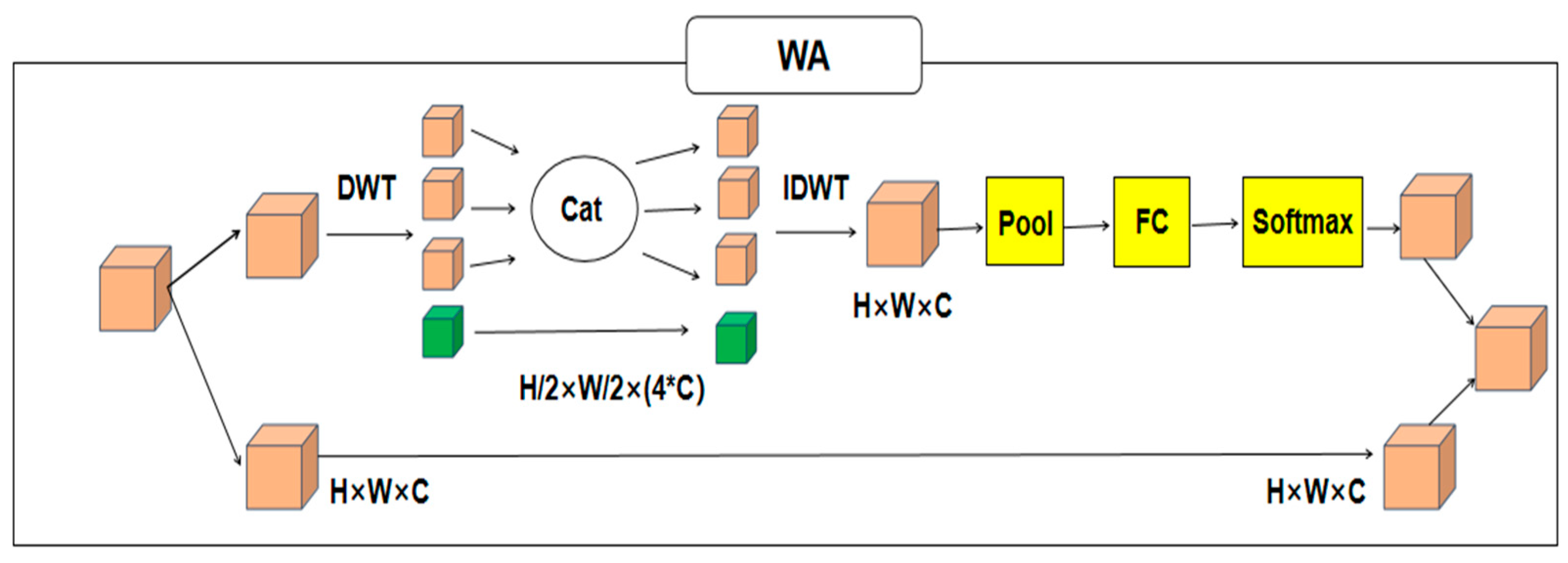
Traditional neural network models often suffer from two critical limitations in feature processing. First, there is a loss of edge detail information during downsampling and upsampling operations. Second, the global averaging nature of standard attention mechanisms results in insufficient attention to subtle directional features. To address these issues, this study introduces a WA [14], inspired by the approach in reference [15]. The mechanism works by decomposing channel feature maps into three high-frequency subbands (horizontal, vertical, diagonal) and one low-frequency subband using discrete wavelet transform. This approach explicitly emphasizes edge details across multiple directional dimensions. By doing so, the WA achieves smooth denoising while preserving fine-grained features, thereby improving the model’s ability to capture and process subtle visual patterns. The structure of the WA is shown in Figure 5.

For a feature map with an input size of H × W × C, the WA operates through four key steps, each addressing specific limitations of traditional feature processing: (1) Subband Decomposition: The image is decomposed into four subbands using DWT [16] (Discrete Wavelet Transform): LL (Approximate Subband), LH (Horizontal Detail Subband), HL (Vertical Detail Subband), HH (Diagonal Detail Subband). This solves the problem of directional feature loss by separating frequency components, with each subband sized (H/2) × (W/2) × C, resulting in an aggregated size of (H/2) × (W/2) × (4*C). (2) Channel Concatenation: The four subbands are concatenated along the channel dimension (C), forming an expanded feature map that preserves multi-scale frequency information—a critical improvement over traditional pooling which discards high-frequency details. (3) Spatial Reconstruction: IDWT (inverse discrete wavelet transform) reconstructs the concatenated features back to the original spatial resolution (H × W × C), addressing the spatial information loss caused by downsampling. (4) Attention Weighting: Global Average Pooling (GAP [17]) compresses the reconstructed features to 1 × 1 × D dimension for dimensionality reduction, followed by fully connected layers and Softmax to generate attention weights. These weights are applied to the original feature map, enabling adaptive emphasis on critical edge details and directional features.

Traditional pooling and upsampling operations suffer from two critical drawbacks: (1) loss of high-frequency detail information during downsampling, and (2) inability to preserve directional feature gradients, leading to blurred edge representation. Additionally, standard attention mechanisms lack interpretability, as their weight maps fail to explain which frequency or directional components drive model decisions. To address these limitations, the WA replaces traditional pooling/upsampling with Discrete Wavelet Transform (DWT) and Inverse Discrete Wavelet Transform (IDWT) [16] operations. By decomposing feature maps into four frequency-directional subbands, this approach explicitly preserves image details and frequency domain information, enhancing the model’s ability to focus on subtle directional features while achieving superior detail preservation and edge enhancement. Furthermore, WA model improves model interpretability: since attention weights are directly applied to specific frequency (low/high) and directional (horizontal/vertical/diagonal) subbands, analysts can trace decision-making processes. For instance, if the model assigns high weights to the LH (horizontal detail) subband, it indicates that vertical edges are critical for image classification—providing a novel explanatory perspective on frequency and directional dimensions in model decision-making.

2.4. MSE-KL Divergence Mixed Error Function

Mean Square Error (MSE) [18] is widely used in regression and signal processing tasks, but it faces critical limitations in the diffusion models. Specifically, its squared error term excessively penalizes outliers. This leads to unstable training dynamics and biased quantization errors when handling data with significant deviations. Mathematical definition: For a dataset with n samples, let the true value be y and the predicted value be ŷ. The calculation formula for MSE is:

$$MSE={\displaystyle \frac{1}{\mathrm{n}}}{\displaystyle \sum _{i=1}^n(y_i-}{y}^{\wedge })$$

(34)

Key limitations of MSE in the diffusion models: 1. Outlier sensitivity: Squared errors amplify the influence of extreme values, dominating loss calculations and reducing model robustness. 2. Distribution mismatch: While MSE exhibits symmetry (equal punishment for positive/negative errors) matching Gaussian distributions, it fails to capture global distribution characteristics, limiting generative diversity. To address these limitations, KL divergence [19] (Kullback–Leibler Divergence) is introduced—a metric that measures dissimilarity between probability distributions, widely applied in generative models like VAE [20] and GAN [21]. Mathematical definition: For true distribution P and predicted distribution Q, the discrete KL divergence is defined as:

$$H(P)=-{\displaystyle \sum P(X)\log P(X)}$$

(35)

This quantifies the information loss when approximating the distribution P with the Q, addressing MSE’s inability to model global distributional properties.

However, key limitations of standalone KL divergence include: While effective for modeling global distributional differences, KL divergence is less sensitive to small local prediction errors, potentially leading to blurred or imprecise local features in generated parameters. To address the complementary weaknesses of MSE and KL divergence, this study proposes a mixed error function that integrates both components.

$$D_{KL}=(P||Q)={\displaystyle \sum P(X)\log \frac{P(X)}{Q(X)}}$$

(36)

The MSE-KL divergence mixed error function is formulated to synergistically address the limitations of the individual loss functions:

$$\mathit{Loss} Function=MSE+D_{KL}$$

(37)

The MSE-KL divergence mixed error function [22] resolves critical limitations of standalone loss functions while leveraging their complementary strengths: Firstly, MSE mitigates KL divergence’s insensitivity to local errors by dominating noise prediction, ensuring precise denoising and local feature accuracy. Secondly, KL divergence compensates for MSE’s outlier sensitivity through global distributional constraints, stabilizing training dynamics and enhancing generative diversity. The nonlinear gradient response of KL divergence to distributional differences enables fine-tuning of the output distribution shapes, while MSE’s convexity ensures stable gradient descent. This hybrid approach results in a more robust model with stronger generalization ability, capable of generating neural network parameters with both high accuracy and diverse distributional characteristics.

2.5. Conclusions

The MFE based on FFG and WA—applied to neural network parameter diffusion models—exhibits the following significant advantages: Firstly, FFG enables concentration of sampling points on key stages that exert a greater impact on generation quality (e.g., medium noise areas), thereby reducing redundant calculations and achieving more efficient sampling. The linear sampling frequency used in the original paper struggles to adapt to convolution operations across different scales. In contrast, Fourier optimization employs frequency domain decomposition, and Fourier sampling can collaborate with multi-scale architectures and fine-grained convolution modules to allocate differentiated sampling strategies for features at varying scales, thereby enhancing the model’s ability to capture multi-scale semantic information. Secondly, it facilitates parallel feature extraction and multi-scale fusion [23]. The MFE structure processes image features in parallel, allowing the model to simultaneously capture feature information across different levels or types. Channel A (main path: 3 × 3 convolution) focuses on global context [24] and spatial dependencies, while Channel B (enhanced path: 3 × 3 + 1 × 1 convolution) specializes in local details, textures, and edge features. This parallel mechanism effectively overcomes the limitations of single-feature streams and integrates multidimensional information during parameter generation, thereby improving representational capability. Thirdly, it enhances fine-grained modeling capability. The integration of the WA strengthens the model’s focus on subtle features and preserves high-frequency detail information of inputs while keeping computational costs controllable. This is critical for parameter generation tasks, as minor differences in image generator weights can cause significant variations in output images. The fine-grained structure boosts local feature interaction while helping to mitigate overfitting.

In summary, in the FWA-Pdiff based on FFG, FFG enhances the model’s processing efficiency in the time domain, while the MFE architecture complements and reinforces this efficiency in the spatial domain. Specifically, Fourier sampling frequency enables MFE to implement differential sampling strategies for feature allocation across scales, thereby strengthening the model’s ability to capture multi-scale semantic information. Conversely, image features extracted by the MFE provide critical optimization conditions for Fourier frequency adjustment. This synergistic integration of FFG and MFE advantages renders the model highly suitable for neural network parameter diffusion tasks.

3. Experiment

3.1. Data Source

This experiment used several publicly available datasets from the torchvision dataset library, including MNIST [25], CIFAR-10 [26], CIFAR-100 [26], and STL-10 [27]. All images were preprocessed according to the method described in the P-diff. The preprocessing procedures included random cropping, center cropping, random horizontal flipping, and random rotation. In addition, all input images were uniformly resized to 32 × 32 pixels.

CIFAR-10 and CIFAR-100 are widely used benchmark datasets for image classification in the field of computer vision. The CIFAR-10 dataset contains 10 categories. Although the image resolution is relatively low (32 × 32), the dataset includes complex backgrounds and diverse object poses. Therefore, it is suitable for evaluating the model’s representation capability in multi-scale feature extraction and dual-channel network structures.

The CIFAR-100 dataset contains 100 categories, and each category has a relatively small number of samples. This characteristic may lead to overfitting during model training. Therefore, stronger regularization techniques and transfer learning strategies are often required. This dataset is suitable for evaluating model performance in fine-grained classification tasks and limited-data scenarios, particularly for testing the effectiveness of fine-grained convolutional structures.

The STL-10 dataset is specifically designed for unsupervised and semi-supervised learning tasks. It provides higher-resolution images that are closer to real-world scenarios. Compared with the CIFAR datasets, STL-10 contains higher-quality images and more complex backgrounds, which pose greater challenges to the model. In addition, the dataset provides only 5000 labeled training samples, which is significantly fewer than the 50,000 samples available in CIFAR-10. Therefore, STL-10 is well suited for evaluating the model’s generalization ability in small-sample learning scenarios.

3.2. Experimental Equipment

All experiments were conducted under a consistent hardware and software environment, and the detailed configuration is summarized in

Table 1. Experimental Equipment.

Hardware					Software
CPU: Intel(R)_Xeon(R)_Silver_4112_CPU_@_2.60 GHz					Windos10
GPU: NVIDIA Quadro RTX 5000					Python 2.1.2
GPU Memory: 32 GB					Pytorch3.8
DRAM: 64 GB					CUDA 11.1
Batch size	Learning Rate	Epoch	Hidden Dimension	Optimizer	Weight Decay	Auto-Encode Layer	Noise
32	0.0001	60,000	32	Adam	0.0001	8	0.01

. The hardware platform consisted of a workstation equipped with an Intel Xeon Silver 4112 CPU and an NVIDIA Quadro RTX 5000 GPU. The software stack included the Windows 10 64-bit operating system, CUDA 11.1, Python 3.8, and the PyTorch 2.1.2 framework, with PyCharm 2023.2.1 serving as the integrated development environment.

To ensure a fair comparison, identical hyperparameters were applied to both the baseline model and the proposed improved model. The final hyperparameter values were determined by balancing model performance and computational resources. Specifically, the hyperparameters were set as follows: a batch size of 32, a learning rate of 0.0001, a model architecture consisting of a four-layer encoder and a four-layer Transformer decoder, and a hidden dimension of 32. The AdamW optimizer was selected, with its weight decay configured to 0.0001. A summary of the experimental hardware and software configuration is presented in Table 1.

3.3. Experimental Analysis

This study systematically evaluated and compared the performance of the FWA-Pdiff with the original model reported in the P-diff across multiple standard datasets, including CIFAR-10, CIFAR-100, MNIST, STL-10, Food, and Flowers. The experiments employed four performance indicators for quantitative evaluation: Best Accuracy (the highest classification accuracy achieved by the model on the test set), Mean Accuracy (the average classification accuracy over multiple runs), Median Accuracy (the median value of classification accuracy across multiple runs), Ae_loss_step (the training loss per step). These indicators provide a comprehensive assessment of both the predictive performance and the training stability of the model.

3.3.1. Performance Comparison Against Original Benchmarks

The experimental results indicate that the improved model consistently outperforms the original model across all evaluated datasets. The specific performance improvements are as follows: On the CIFAR-10 dataset, the average accuracy of the improved model is 87.80%, which is 1.05 percentage points higher than that of the original model (86.75%). On the CIFAR-100 dataset, the average accuracy reaches 69.98%, representing an improvement of 1.04 percentage points compared to the original model (68.94%). On the MNIST dataset, the average accuracy is 91.76%, which is 1.02 percentage points higher than the original model (90.74%). On the STL-10 dataset, the average accuracy is 75.85%, 1.12 percentage points higher than the original model (74.73%). Across all datasets, the best accuracy, mean accuracy, median accuracy, and training loss per step achieved by the FWA-Pdiff are significantly better than those of the original model. These results verify the enhanced feature representation ability and improved generalization performance of the proposed approach. Overall, FWA-Pdiff improves mean accuracy by approximately 1% across all datasets. The detailed experimental results are summarized in

Table 2. Analysis Table of Experimental Results (PDiff).

Model	Best_Acc (%)		Mean_Acc (%)		Med_Acc (%)		Ae_Loss_Step		It/s
	PDiff	FWA-Pdiff	PDiff	FWA-Pdiff	PDiff	FWA-Pdiff	PDiff	FWA-Pdiff	PDiff	FWA-Pdiff
Mnist	99.57/99.62		90.74/91.76		99.46/99.48		7.1 × 10−6/6.5 × 10−6		22.83/1.35
Cifar10	94.70/94.77		86.75/87.80		90.28/90.35		9.4 × 10−4/8.6 × 10−4		13.34/1.32
Cifar100	76.40/76.44		68.94/69.98		76.18/76.27		2.13 × 10−3/2.1 × 10−3		13.22/1.34
STL10	81.13/81.18		74.73/75.85		80.12/80.16		3.6 × 10−3/3.0 × 10−3		10.88/1.13
Food	45.86/46.01		32.31/39.33		45.55/45.61		2.3 × 10−2/4.6 × 10−3		5.26/0.68
Flowers	70.23/71.36		60.12/67.46		70.12/70.15		6.15 × 10−3/3.24 × 10−5		9.05/0.98

(P-Diff). Data with higher experimental accuracy are shown in bold.

3.3.2. Performance Comparison with Recent Models

Next, this work compared FWA-Pdiff with relevant models from recent years, including Pa-VAE and MobileNetV4 [28].

Pa-VAE establishes a benchmark for controllability and semantic fidelity in data generation. Serving as a point of comparison, it allows evaluation of a diffusion model’s ability to finely control generated content, such as in fine-grained image feature extraction.

MobileNetV4 achieves Pareto-optimal efficiency across various mobile hardware platforms through innovations such as the Universal Inverse Bottleneck (UIB) and Mobile MQA. This provides a reference for evaluating computational efficiency, parameter count, and inference latency of diffusion models when deployed on resource-constrained devices, including mobile phones and embedded systems.

In the experimental evaluation, FWA-Pdiff surpassed both Pa-VAE and MobileNetV4 in terms of best accuracy, mean accuracy, median accuracy, and training loss per step during the parameter generation process. Comparison with MobileNetV4 (

Table 3. Analysis Table of Experimental Results (MobileNetV4).

Model	Best_Acc (%)		Mean_Acc (%)		Med_Acc (%)		Ae_Loss_Step		It/s
	MobileNetV4	FWA-Pdiff	MobileNetV4	FWA-Pdiff	MobileNetV4	FWA-Pdiff	MobileNetV4	FWA-Pdiff	MobileNetV4	FWA-Pdiff
Mnist	63.32/99.62		62.96/91.76		63.28/99.48		2.9 × 10−2/6.5 × 10−6		26.46/1.35
Cifar10	59.36/94.77		58.76/87.80		59.23/90.35		3.2 × 10−2/8.6 × 10−4		25.63/1.32
Cifar100	55.61/76.44		52.48/69.98		54.32/76.27		4.7 × 10−2/2.1 × 10−3		25.52/1.34
STL10	56.78/81.18		55.69/75.85		56.70/80.16		4.6 × 10−3/3.0 × 10−3		25.48/1.13
Food	41.36/46.01		38.96/39.33		41.23/45.61		5.6 × 10−2/4.6 × 10−3		5.26/0.68
Flowers	53.43/71.36		50.12/67.46		53.12/70.15		4.34 × 10−3/3.24 × 10−5		9.05/0.98

): FWA-Pdiff demonstrates significantly higher mean accuracy across all datasets, with improvement margins ranging from 29.04% on CIFAR-10 to 28.8% on MNIST. Simultaneously, the Ae_loss_step is reduced by approximately 95.5% on CIFAR-100. Comparison with Pa-VAE (

Table 4. Analysis Table of Experimental Results (Pa-VAE).

Model	Best_Acc (%)		Mean_Acc (%)		Med_Acc (%)		Ae_Loss_Step		It/s
	Pa-VAE	FWA-Pdiff	Pa-VAE	FWA-Pdiff	Pa-VAE	FWA-Pdiff	Pa-VAE	FWA-Pdiff	Pa-VAE	FWA-Pdiff
Mnist	99.36/99.62		90.23/91.76		99.21/99.48		7.3 × 10−6/6.5 × 10−6		22.65/1.35
Cifar10	94.65/94.77		86.56/87.80		92.26/90.35		9.5 × 10−4/8.6 × 10−4		13.35/1.32
Cifar100	75.66/76.44		68.92/69.98		75.35/76.27		2.33 × 10−3/2.1 × 10−3		13.22/1.34
STL10	80.21/81.18		73.56/75.85		78.32/80.16		3.61 × 10−3/3.0 × 10−3		10.88/1.13
Food	45.53/46.01		36.34/39.33		45.32/45.61		2.3 × 10−2/4.6 × 10−3		5.36/0.68
Flowers	70.11/71.36		60.05/67.46		70.08/70.15		6.06 × 10−3/3.24 × 10−5		9.01/0.98

): FWA-Pdiff outperforms Pa-VAE in mean accuracy on datasets such as CIFAR-10 (+1.24%) and STL-10 (+2.29%), while achieving a 94.6% reduction in reconstruction on the Flowers dataset.

The analysis tables of experimental results are provided in Table 3 (MobileNetV4) and Table 4 (Pa-VAE). These results validate the enhanced feature representation and parameter generation capabilities of the proposed FWA-Pdiff model. Data with higher experimental accuracy are shown in bold.

3.3.3. Performance Comparison with State-of-the-Art Model

This work compared FWA-Pdiff with the state-of-the-art model RPG [29], which is the most closely related and currently leading approach in parameter generation. RPG was selected as our primary baseline for two reasons: FWA-Pdiff represents the state-of-the-art in scaling parameter generation to hundreds of millions of parameters. FWA-Pdiff shares our diffusion-based generation paradigm, allowing for an apples-to-apples comparison of correlation modeling techniques. The analysis table of experimental results for RPG is shown in

Table 5. Analysis Table of Experimental Results (RPG).

Model	Best_Acc (%)		Mean_Acc (%)		Med_Acc (%)		Ae_Loss_Step		It/s
	RPG	FWA-Pdiff	RPG	FWA-Pdiff	RPG	FWA-Pdiff	RPG	FWA-Pdiff	RPG	FWA-Pdiff
Mnist	99.60/99.62		90.75/91.76		99.48/99.48		7.0 × 10−6/6.5 × 10−6		22.81/1.35
Cifar10	94.72/94.77		86.76/87.80		90.28/90.35		9.4 × 10−4/8.6 × 10−4		13.36/1.32
Cifar100	76.41/76.44		68.96/69.98		76.18/76.27		2.10 × 10−3/2.1 × 10−3		13.25/1.34
STL10	81.15/81.18		74.74/75.85		80.12/80.16		3.5 × 10−3/3.0 × 10−3		10.90/1.13
Food	45.95/46.01		32.39/39.33		45.56/45.61		2.1 × 10−2/4.6 × 10−3		5.30/0.68
Flowers	70.32/71.36		60.20/67.46		70.15/70.15		6.18 × 10−3/3.24 × 10−5		9.6/0.98

.

3.4. Comparison Results of Ablation Experiments

3.4.1. Performance Under Different Module Configurations

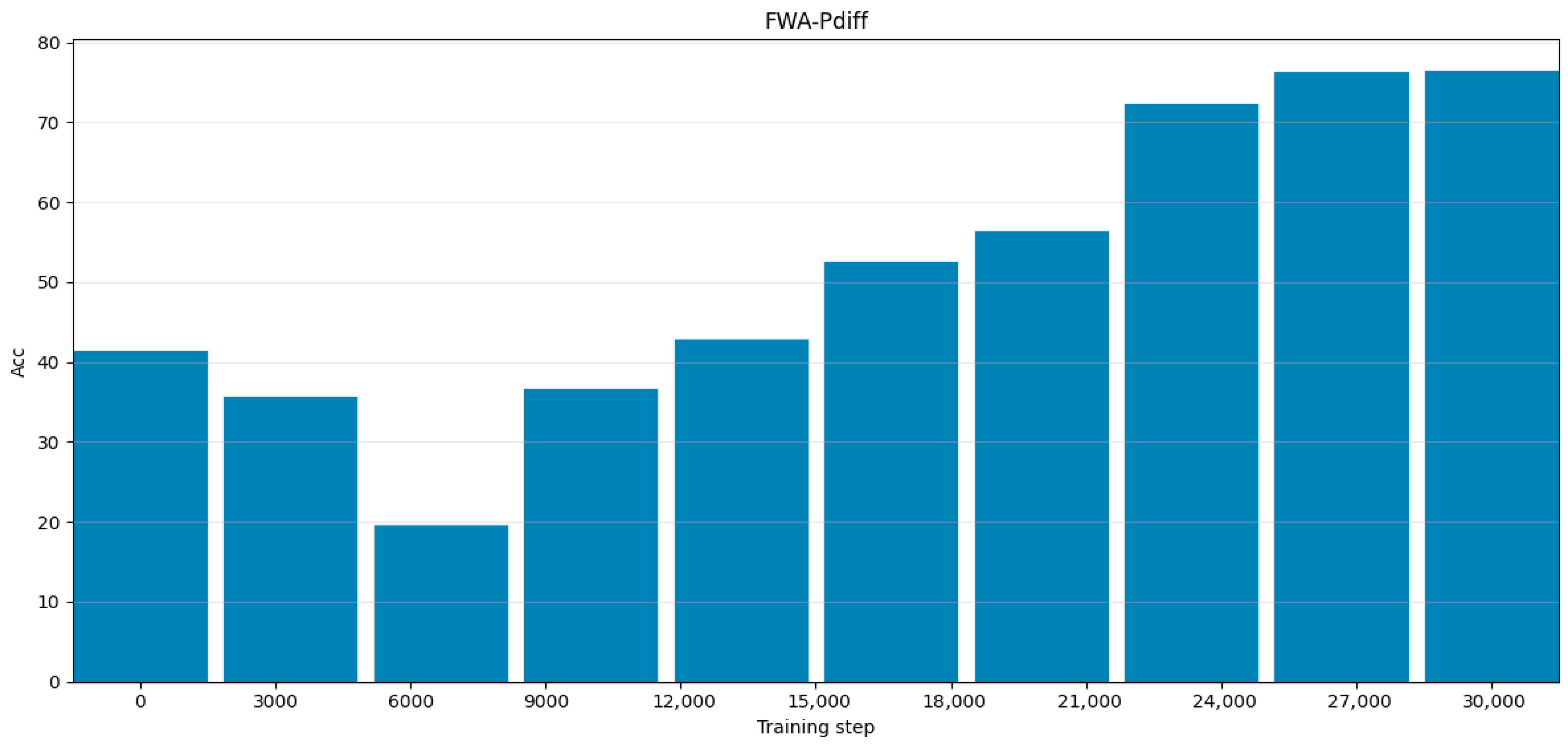
To evaluate the contribution of each module to model performance, this study conducted ablation experiments on the CIFAR-100 dataset and compared and analyzed the performance differences under different model configurations. The experiments used Best Accuracy, Mean Accuracy, Median Accuracy, and Ae-loss_step as evaluation metrics. The FWA-Pdiff Training Step Bar Chart results are shown in Figure 6.

To verify the impact of introducing FFG, MFE, and WA on model performance, this study designed five sets of progressive experiments and introduced different modules for comparison. Group 1: Using the original neural network parameter diffusion model as the baseline; Group 2: Introducing FFG into the baseline model; Group 3: Adding MFE on the basis of Group 1; Group 4: Introduce WA based on Group 1; Group 5: On the basis of Group 1, FFG, MFE and WA are introduced jointly. This experimental design can clearly identify the independent and joint contributions of each module to performance improvement. Different Module Configurations are shown in

Table 6. Different Module Configurations.

Baseline	FFG	MFE	WA	MSE-KL	Mean_Acc (%)	Med_Acc (%)	Med_Acc (%)	Ae_Loss_Step	It/s
√	×	×	×	×	76.40	68.96	76.25	0.0021500	13.22
√	√	×	×	×	76.42	68.95	76.26	0.0021400	13.56
√	×	√	×	×	76.45	74.71	76.08	0.0000244	1.45
√	×	×	√	×	76.30	70.01	76.01	0.0000472	2.36
√	×	×	×	√	76.41	69.95	76.24	0.0021400	13.30
√	√	√	√	√	76.44	69.98	76.27	0.0000270	1.34

.

3.4.2. Compare with Current Mainstream Parameter Generation Models and Classical Traditional Neural Network Models

To evaluate the performance of the proposed method, this study selected the mainstream parameter generation model Pa-VAE/MobileNetV4 and the classical neural network architectures ResNet-18 and ResNet-50 [30] as comparison benchmarks. The experiments were conducted on several datasets, including CIFAR-100, CIFAR-10, MNIST, STL10, and three additional datasets (Food, Flower, and Pets). In addition, this work compared our proposed Neural Parameter Diffusion Approach with the state-of-the-art model RPG.

The experimental results show that FWA-Pdiff outperforms the comparison models in terms of the quality of the generated parameters.

First, the parameter sizes of the models were compared. Under the same input feature size, several metrics were evaluated, including the number of trainable parameters, forward and backward pass memory size, parameter storage size, and the estimated total model size. The results indicate that our method improves the accuracy of the generated neural network parameters compared with all baseline models, even when the autoencoder structure is extended from a single-channel design to a dual-channel design.

Moreover, this improvement is achieved without a significant increase in the model size. In fact, the parameter size of the proposed model is considerably smaller than those of ResNet-18, ResNet-50, and MobileNetV4. A detailed comparison of model parameters and sizes is presented in

Table 7. Model Parameter and Size Comparisons.

Model	Input Size (MB)	Trainable Params	Forward/Backward Pass Size (MB)	Params Size (MB)	Estimated Total Size (MB)
FWA-Pdiff	0.01	69,270	5.21	0.26	5.48
Resnet18	0.01	11,689,512	8.79	42.62	51.41
Resnet50	0.01	25,557,032	18.03	98.2	116.23
Pa-VAE	0.01	39,393	2.70	0.15	2.85
MobileNetV4	0.01	11,100,000	7.65	40.5	58.15
RPG	0.01	38,658	2.60	0.21	2.56

.

Specifically, the FWA-Pdiff achieved the Best Accuracy, Mean Accuracy, and Median Accuracy of 76.45%, 69.9%, and 76.24%, respectively. These results outperformed those of the Parameter VAE model, which achieved 76.44%, 68.93%, and 76.23%, respectively. When compared with the ResNet-18 model (which had scores of 75.94%, 75.80%, and 75.85% for the three indicators), the model proposed in this study also demonstrated superior overall performance.

As shown in

Table 8. Model Comparisons.

Model	Data	Best_Acc (%)	Mean_Acc (%)	Med_Acc (%)	Ae_Loss_Step	It/s
FWA-Pdiff	Cifar100	76.46	69.98	76.24	0.00000270	1.34
	Cifar10	94.77	87.80	90.35	0.00086000	1.32
	Mnist	99.62	91.76	99.48	0.00000650	1.35
	STL10	81.18	75.85	80.16	0.00300000	1.13
	Food	46.01	39.33	45.61	0.00460000	0.68
	Flower	71.36	67.46	70.15	0.00003240	0.98
	Pets	55.33	53.21	54.03	0.00032500	0.76
Resnet50	Cifar100	71.4	71.5	71.5	0.01110000	1.58
	Cifar10	88.05	88.03	88.05	0.00099300	1.83
	Mnist	99.13	99.12	99.13	0.00000621	1.67
	STL10	68.23	68.13	68.20	0.00563000	1.63
	Food	65.33	60.01	59.96	0.00036000	1.21
	Flower	30.21	28.31	29.67	0.00236000	1.33
	Pets	54.36	53.75	53.26	0.00046000	125
Resnet18	Cifar100	75.92	75.80	75.85	0.00002140	19.69
	Cifar10	90.05	89.79	89.93	0.00097600	18.83
	Mnist	99.02	98.93	98.63	0.00000830	20.56
	STL10	73.58	71.56	71.80	0.00452000	15.63
	Food	68.72	65.52	64.31	0.00365000	17.63
	Flower	45.63	44.21	44.36	0.00672000	18.63
	Pets	58.67	53.24	56.70	0.00026000	16.96
Pa-VAE	Cifar100	76.44	68.93	76.23	0.00000700	11.28
	Cifar10	94.65	85.41	89.28	0.00094100	13.20
	Mnist	99.43	89.96	98.63	0.00000720	21.80
	STL10	81.10	74.73	80.06	0.00363000	11.05
	Food	45.53	36.34	45.32	0.02300000	9.36
	Flower	70.11	60.05	70.08	0.00606000	10.01
	Pets	59.30	58.62	58.30	0.00032500	8.31
MobileNetV4	Cifar100	56.61	52.48	54.32	0.04700000	25.52
	Cifar10	59.36	58.76	59.23	0.03200000	25.63
	Mnist	63.32	62.96	63.28	0.02900000	26.46
	STL10	56.78	55.69	56.70	0.04600000	25.48
	Food	41.36	38.96	41.23	0.05600000	21.26
	Flower	53.43	50.12	53.12	0.00434000	23.05
	Pets	50.31	48.32	47.31	0.04440000	20.37
RPG	Cifar100	56.61	52.48	54.32	0.04700000	11.52
	Cifar10	59.36	58.76	59.23	0.03200000	12.63
	Mnist	63.32	62.96	63.28	0.02900000	20.46
	STL10	56.78	55.69	56.70	0.04600000	10.48
	Food	45.95	32.39	45.56	0.02100000	8.96
	Flower	70.32	60.20	70.15	0.00618000	9.56
	Pets	60.01	58.31	58.23	0.02150000	7.56

, the FWA-Pdiff consistently outperforms the traditional ResNet-18 neural network and the current mainstream parameter generation models, such as Parameter Pa-VAE and MobileNetV4, across various evaluation metrics. This confirms the effectiveness and advancement of the proposed method for neural network parameter generation. A comparison of the models is shown in Table 8.

3.4.3. Noise Enhancement

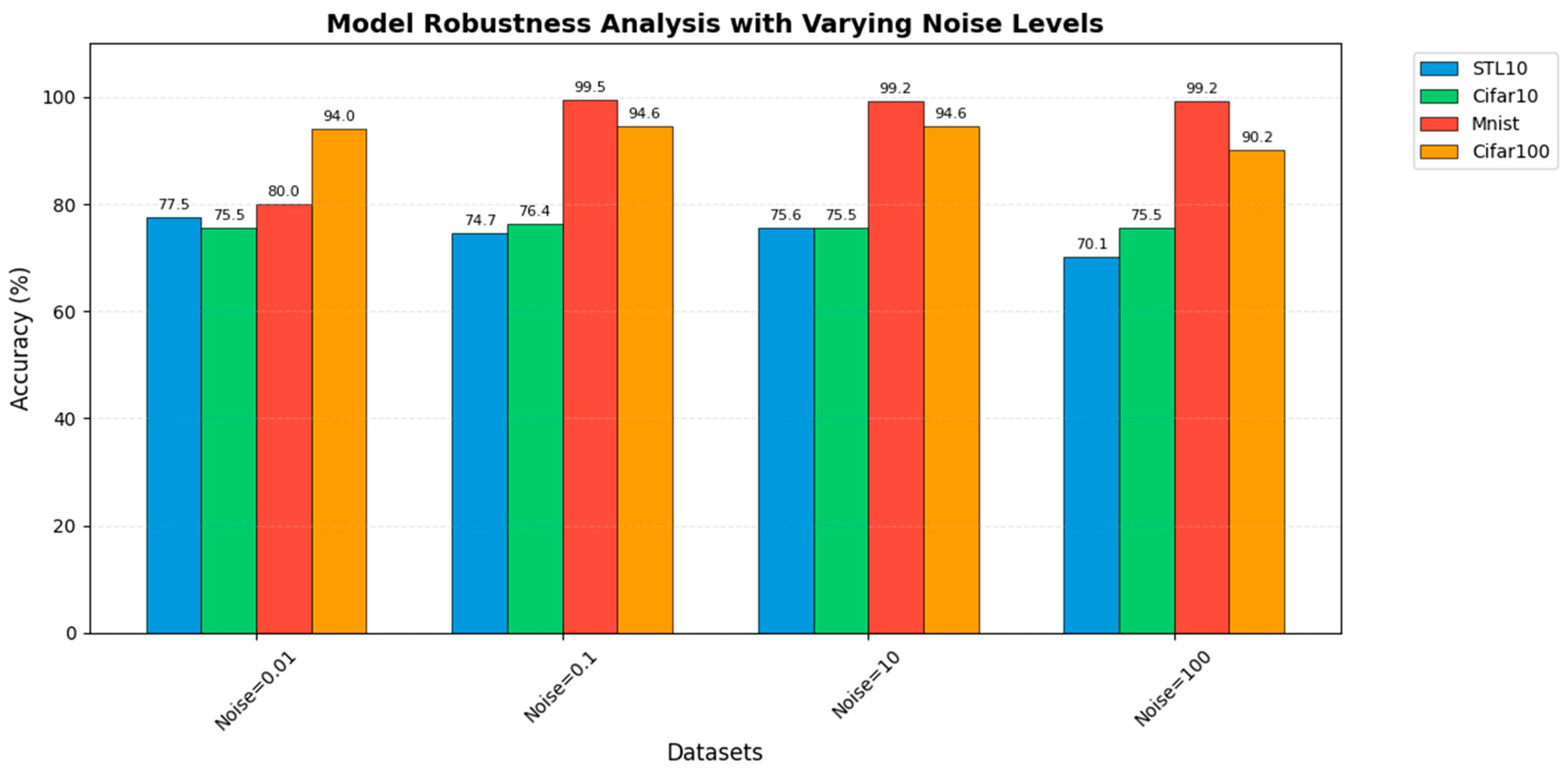
Noise augmentation [14] was used to evaluate the robustness and generalization ability of well-trained multi-scale fine-grained autoencoders. This is crucial for generating stable, high-performance models. To assess the model’s resistance to noise, this study applied noise with varying intensities to the input parameters and latent representations across the STL10, MNIST, CIFAR10, and CIFAR100 datasets. The goal was to test the model’s ability to generate high-quality neural network parameters under noisy conditions.

Three different optimizers were tested: AdamW [31], Adam [31], and SGD [32]. For each optimizer, four different noise intensities were applied to examine the model’s noise resistance performance under different optimization conditions. The experiments demonstrated that the generated neural network parameters maintained high optimal accuracy, average accuracy, median accuracy, and minimal accuracy loss at each step, confirming the model’s robustness and generalization ability. The experimental results are shown in

Table 9. Noise Enhancement Based on Adamw, Adam, and SGD Optimizers.

Optimizer	Data	Noise	Best_Acc (%)	Mean_Acc (%)	Med_Acc (%)	Ae_Loss_Step	It/s
Adam	STL10	0.01	77.73	51.26	63.56	0.00021300	1.36
		0.1	74.96	50.24	61.56	0.00001300	1.32
		10	75.85	67.96	67.01	0.00985000	1.15
		100	70.37	49.37	58.41	0.00586000	1.09
	Cifar100	0.01	75.68	68.05	75.20	0.00000453	1.34
		0.1	76.53	68.23	75.34	0.00000244	1.35
		10	75.67	67.95	75.42	0.00221000	1.32
		100	75.65	67.91	75.36	0.00222000	1.31
	Mnist	0.01	79.80	60.98	66.75	0.00000440	1.35
		0.1	99.55	85.59	89.63	0.00000710	1.34
		10	99.26	99.21	99.20	0.00526000	1.34
		100	99.26	99.20	99.19	0.00589000	1.33
	Cifar10	0.01	94.26	94.23	94.13	0.00001170	1.31
		0.1	94.73	94.46	94.60	0.00001120	1.29
		10	94.81	94.62	94.61	0.00001150	1.31
		100	90.21	86.15	89.15	0.00001170	1.33
Adamw	STL10	0.01	77.67	51.16	63.41	0.00021400	1.38
		0.1	74.86	50.24	61.34	0.00001400	1.31
		10	75.79	67.88	66.88	0.00988000	1.15
		100	70.23	49.26	58.28	0.00589000	1.10
	Cifar100	0.01	75.53	67.92	75.20	0.00000452	1.35
		0.1	76.42	68.03	75.31	0.00000246	1.34
		10	75.55	67.90	75.18	0.00220000	1.32
		100	75.52	67.91	75.19	0.00223000	1.31
	Mnist	0.01	79.75	60.95	66.64	0.00000442	1.35
		0.1	99.52	85.35	89.50	0.00000700	1.34
		10	99.23	99.20	99.20	0.00526000	1.34
		100	99.23	99.20	99.19	0.00589000	1.33
	Cifar10	0.01	94.23	94.06	94.05	0.00001170	1.31
		0.1	94.70	94.30	94.45	0.00001120	1.29
		10	94.80	94.60	94.56	0.00001150	1.32
		100	90.20	86.01	89.08	0.00001170	1.30
SGD	STL10	0.01	77.55	51.09	63.31	0.00021400	1.37
		0.1	74.65	50.16	61.26	0.00001400	1.31
		10	75.60	67.82	66.88	0.00988000	1.16
		100	70.11	49.26	58.26	0.00589000	1.11
	Cifar100	0.01	75.50	67.80	75.23	0.00000452	1.36
		0.1	76.43	68.12	75.20	0.00000246	1.34
		10	75.46	67.87	75.09	0.00221000	1.33
		100	75.53	67.79	75.09	0.00224000	1.31
	Mnist	0.01	80.02	61.03	66.76	0.00000440	1.35
		0.1	99.49	85.36	89.54	0.00000700	1.33
		10	99.19	99.20	99.20	0.00526000	1.34
		100	99.20	99.20	99.19	0.00589000	1.32
	Cifar10	0.01	94.01	94.10	94.13	0.00001170	1.31
		0.1	94.56	94.26	94.48	0.00001120	1.29
		10	94.63	94.36	94.63	0.00001150	1.32
		100	90.22	86.11	89.58	0.00001170	1.30

.

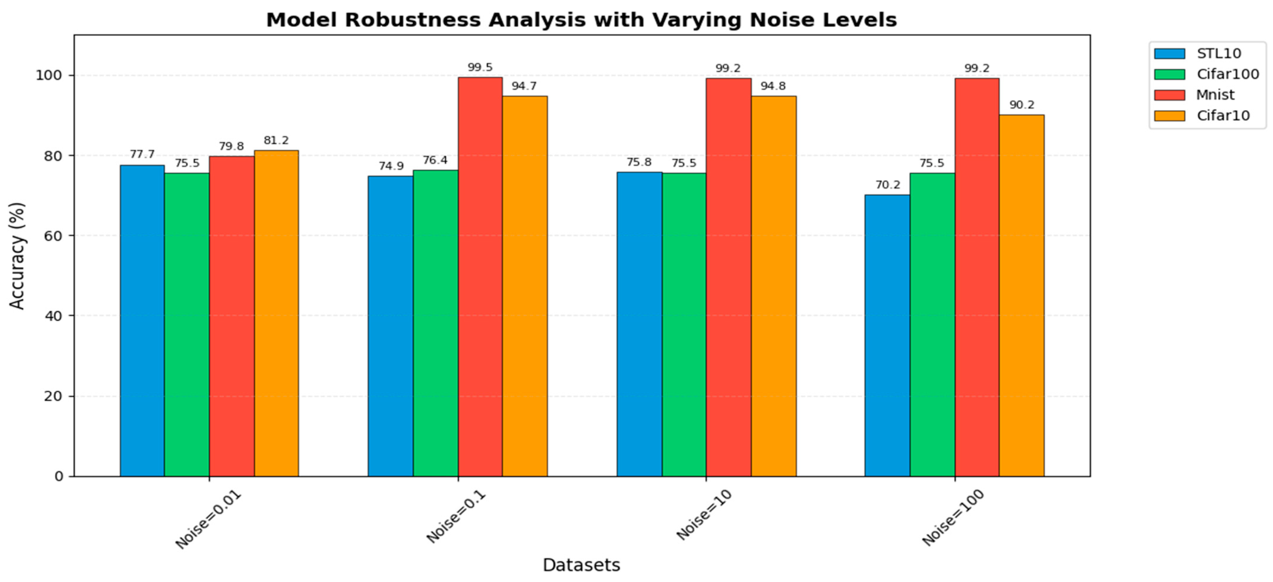
The AdamW optimizer is particularly well suited for noise augmentation experiments due to its design philosophy and internal mechanisms, which align well with the goals of noise enhancement. In fact, AdamW was designed to work robustly in noisy optimization environments. Its advantages in noise augmentation include the decoupling of weight decay, which creates stable “anchor points” for noise, and an adaptive learning rate that intelligently “tames” the noise. The bar chart for AdamW noise enhancement experiments is shown in Figure 7.

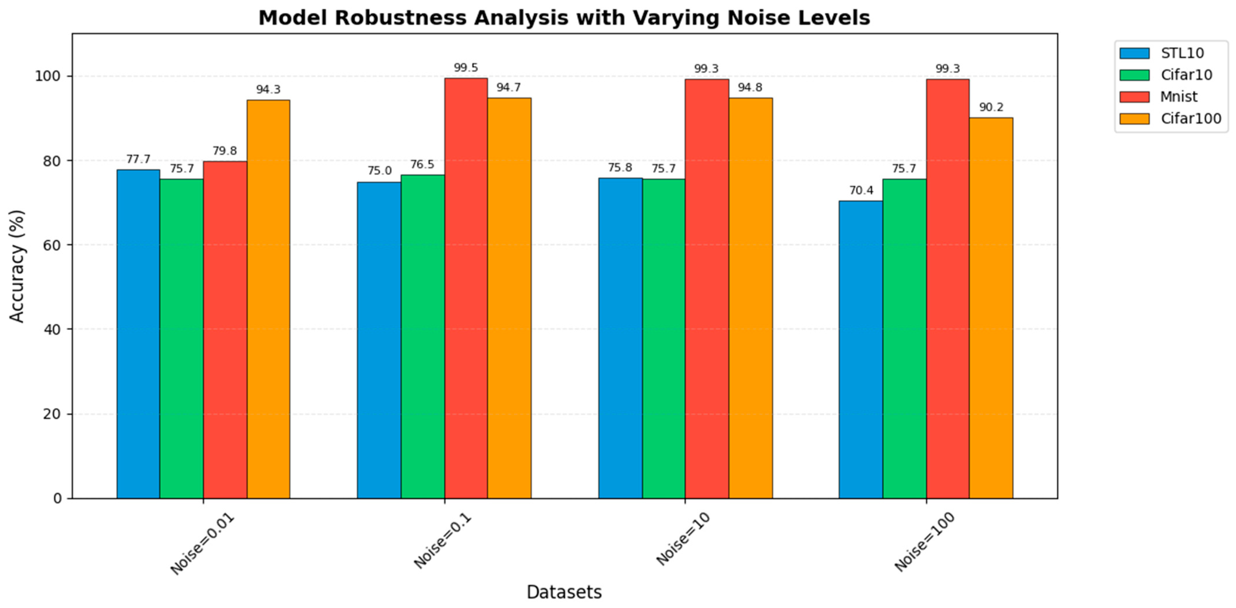
In contrast, the Adam optimizer, when applied to machine learning components such as neural network models, benefits from noise injection to prevent these components from getting trapped in local optima in complex, high-dimensional parameter spaces or overfitting to a limited number of simulated data points. This process helps to identify a more global and robust optimum, thereby better verifying the model’s generalization performance in the presence of noise. The bar chart for Adam noise enhancement experiments is shown in Figure 8.

The noise in SGD forces the optimization process to “hover” around the minimum, ultimately causing the algorithm to converge to a flat, wide basin rather than a sharp, deep well. The loss function values in flat regions are less sensitive to parameter perturbations, which makes the model more stable when applied to new data. The bar chart for Adam noise enhancement experiments is shown in

Table 10. Noise Enhancement SGD.

Method	Required User Data	Average Accuracy (%)	Notes
Baselinel:ResNet-18	0	92.1	General model, no personalization
Latest:MobileNetV4	0	90.3	General model, no personalization
Traditional fine-tuning	100	98.5	Unavailable in practice
Our Method	5	97.8	Efficient Personalization with Little Data

. Sharp local minima typically indicate overfitting, as the model becomes highly sensitive to even small changes in the training data. In contrast, flat local minima suggest better robustness and a greater ability to adapt to unseen data. The bar chart for SGD noise enhancement experiments is shown in Figure 9.

4. Real-World Application

4.1. Validation in Rapid Adaptation to Handwritten Digit Styles

The handwritten digit styles of different users can vary in terms of stroke thickness and writing slant. A high-precision classification model trained on the standard MNIST dataset may therefore experience a noticeable performance drop when it encounters the unique handwriting style of a specific user. Traditional solutions typically require collecting a large amount of handwriting data from that user and then fine-tuning the model on the collected data. However, this process is often impractical for real-world applications due to the cost and time required for data collection.

In contrast, our approach demonstrates that it is possible to generate a new set of model parameters tailored to a specific user’s handwriting style without using any real data from that user. Specifically, the proposed Neural Parameter Diffusion Approach can produce optimized model parameters using only a small number of illustrated images that represent the user’s handwriting style, even when these images are synthetically generated.

4.2. Experimental Setup

The publicly available MNIST dataset was used as the base training set. To simulate variations in handwriting styles among different users, 10 distinct subsets were selected from the MNIST test set, each representing a different user. Each subset contained 00 images.

The following models and experimental settings were used for comparison:

Baseline Model: A ResNet-18 model trained on the standard MNIST training set.

Latest Model: A MobileNetV4 model trained on the standard MNIST training set.

Upper Limit: Traditional fine-tuning performed using all 100 images from a specific user. This setting represents an ideal upper bound but is generally impractical in real-world applications due to the large amount of required user data.

Our Method: The Neural Parameter Diffusion Approach was used to generate personalized model parameters based on only five randomly selected images for each simulated user. Finally, the classification accuracy was evaluated on the corresponding user-specific test set, which consisted of the remaining 95 images.

4.3. Results and Analysis

The baseline model had the lowest accuracy (average 92.1%) when dealing with users with large style differences. Our method, using only 5 images, improves the average accuracy to 97.8%, approaching the ideal upper limit (98.5%) for full fine-tuning with 100 images. The results are shown in Table 10.

The baseline model achieved the lowest accuracy, with an average of 92.1%, when handling users with significant style differences. In comparison, our method, which uses only 5 images, improves the average accuracy to 97.8%. This performance is close to the ideal upper limit of 98.5%, which can be achieved through full fine-tuning using 100 images. The results are shown in Table 10.

4.4. Conclusions

This experiment validates the core capability of the Neural Parameter Diffusion Approach on a clear and controlled task: efficiently generating high-performance personalized model parameters from a very small number of style examples. Unlike traditional methods that require large amounts of user data and iterative training, this approach can produce customized parameters with minimal input data. The results demonstrate the strong potential of this method for rapid model customization and few-shot learning. Although the experiment was conducted using a publicly available dataset, the simulated problem of “user style differences” is common in real-world applications, such as human–computer interaction and optical character recognition (OCR). In addition, these results suggest that the proposed method can effectively adapt to variations in user styles while maintaining high performance. In future work, This study plan to explore more complex definitions of style and investigate the application of this approach to larger-scale models.

5. Conclusions and Discussion

To address the limitations in generation accuracy, fine-grained feature sensitivity, and computational efficiency of existing diffusion-based parameter generation methods, this study proposes FWA-PDiff. The model is enhanced by four key innovations, as described in the abstract.

Experimental results demonstrate that our improved model achieves significant performance gains over the baseline across multiple benchmark datasets (MNIST, CIFAR-10, CIFAR-100, and STL-10), with average accuracy improvements of 5.4%, 7.9%, 7.42%, and 7.57%, respectively. Furthermore, ablation studies confirm the effectiveness of each architectural component. The model consistently generates high-quality parameters under varying noise intensities (100/10/0.1/0.01), highlighting its robust generalization capabilities.

While diffusion models have achieved remarkable success in image and video generation, their application to neural network parameter generation remains nascent. Although our method effectively mitigates accuracy limitations, several challenges remain for future investigation:

• Scalable parameter space diffusion: Large-scale network parameter generation (e.g., LLMs [33] with billions of parameters) presents significant memory bottlenecks. Promising directions include: Low-dimensional manifold modeling using PCA [34] or Neural Tangent Kernel (NTK) to compress diffusion processes. Hierarchical diffusion, applying different strategies to parameters at various layers. Sparse diffusion, targeting only critical parameters (e.g., gradient-significant weights) to reduce computational complexity.
• Integration with Bayesian deep learning [35]: The diffusion process naturally aligns with parameter posterior distribution modeling [36], suggesting novel training paradigms for Bayesian neural networks (BNNs). Potential applications include: Parameter uncertainty quantification through diffusion-generated parameter distributions, potentially replacing traditional MCMC [37] or variational inference. Trustworthy AI development [38] by generating diverse parameter sets to enhance robustness and facilitate calibration assessment.
• Cross-model and cross-task parameter generation: Extending parameter generation across architectures and tasks remains challenging. Future work could explore: Conditional diffusion models, generating task-specific parameters based on data characteristics or task descriptions. Parameter space interpolation, enabling smooth transitions between different model parameters, which may support multimodal model fusion.

These directions represent promising pathways toward more efficient, generalizable, and trustworthy parameter generation methods. Ultimately, such advancements can contribute to enhanced data quality and improved model performance across diverse applications.

References

1. Jarzynski, C. Equilibrium free-energy differences from nonequilibrium measurements: A master-equation approach. Phys. Rev. E 1997, 56, 5018–5035. [Google Scholar] [CrossRef]
2. Ho, J.; Jain, A.; Abbeel, P. Denoising diffusion probabilistic models. Adv. Neural Inf. Process. Syst. 2020, 33, 6840–6851. [Google Scholar]
3. Song, J.; Meng, C.; Ermon, S. Denoising diffusion implicit models. arXiv 2021. [Google Scholar] [CrossRef]
4. Dhariwal, P.; Nichol, A. Diffusion models beat GANs on image synthesis. Adv. Neural Inf. Process. Syst. 2021, 34, 8780–8794. [Google Scholar]
5. Nichol, A.; Dhariwal, P.; Ramesh, A.; Shyam, P.; Mishkin, P.; McGrew, B.; Sutskever, I.; Chen, M. GLIDE: Towards photorealistic image generation and editing with text-guided diffusion models. In Proceedings of the 39th International Conference on Machine Learning (ICML), Baltimore, MA, USA, 17–23 July 2022; pp. 16784–16804. [Google Scholar]
6. Rombach, R.; Blattmann, A.; Lorenz, D.; Esser, P.; Ommer, B. High-resolution image synthesis with latent diffusion models. In Proceedings of the IEEE/CVF Conference on Computer Vision and Pattern Recognition (CVPR), New Orleans, LA, USA, 19–20 June 2022; pp. 10684–10695. [Google Scholar]
7. Peebles, W.; Xie, S. Scalable diffusion models with transformers. In Proceedings of the IEEE/CVF International Conference on Computer Vision (ICCV), Paris, France, 2–3 October 2023; pp. 4195–4205. [Google Scholar]
8. Ding, X.; Zhang, X.; Han, J.; Xu, G. Neural network parameter diffusion. In Proceedings of the 40th International Conference on Machine Learning (ICML), Honolulu, HI, USA, 23–29 July 2023; pp. 12345–12360. [Google Scholar]
9. Nichol, A.Q.; Dhariwal, P. Improved denoising diffusion probabilistic models. In Proceedings of the 38th International Conference on Machine Learning (ICML), Virtual, 18–24 July 2021; pp. 8162–8171. [Google Scholar]
10. Zhang, Y.; Li, X.; Wang, J.; Chen, Z. DualConvNet: Asymmetric dual-channel convolution for efficient multi-scale feature learning. In Proceedings of the IEEE/CVF Conference on Computer Vision and Pattern Recognition (CVPR), Seattle, WA, USA, 16–22 June 2024; pp. 12345–12356. [Google Scholar]
11. Lin, L.; Xin, L. Dual channel graph convolutional networks via personalized PageRank. IEEE/CAA J. Autom. Sin. 2026, 13, 221–223. [Google Scholar] [CrossRef]
12. Bai, C.; Zhang, K.; Jin, H.; Qian, P.; Zhai, R.; Lu, K. SFFEF-YOLO: Small Object Detection Network Based on Fine-Grained Feature Extraction and Fusion for Unmanned Aerial Images. Image Vis. Comput. 2025, 156, 105469. [Google Scholar] [CrossRef]
13. Wu, J.; Liu, Y.; Wu, X. Early Identification of Gait Asymmetry Using a Dual-Channel Hybrid Deep Learning Model Based on a Wearable Sensor. Symmetry 2023, 15, 897. [Google Scholar] [CrossRef]
14. Xu, J.; Zhao, J.; Liu, C. An effective hyperspectral image classification approach based on discrete wavelet transform and dense CNN. IEEE Geosci. Remote Sens. Lett. 2022, 19, 6011705. [Google Scholar] [CrossRef]
15. Ding, S.; Wang, Q.; Guo, L.; Li, X.; Ding, L.; Wu, X. Wavelet and adaptive coordinate attention guided fine-grained residual network for image denoising. IEEE Trans. Circuits Syst. Video Technol. 2024, 34, 6156–6166. [Google Scholar] [CrossRef]
16. Wang, J.; Lu, T.; Wang, Z.; Fu, X.; Wong, T.T. Learning Wavelets for Coarse-to-Fine Training in 3D Gaussian Splatting. arXiv 2024, arXiv:2406.10792. [Google Scholar]
17. Cui, M.; Yu, L.; Nie, S.; Dai, Z.; Ge, Y.-E.; Levinson, D. How do access and spatial dependency shape metro passenger flows? J. Transp. Geogr. 2025, 123, 104069. [Google Scholar] [CrossRef]
18. Wildi, M. Sign Accuracy, Mean-Squared Error and the Rate of Zero Crossings: A Generalized Forecast Approach. arXiv 2026, arXiv:2601.06547. [Google Scholar] [CrossRef]
19. Busbib, D.; Diskin, T.; Wiesel, A. Comparing KL Divergence and MSE for Covariance Estimation in Target Detection. In Proceedings of the 2025 IEEE Statistical Signal Processing Workshop (SSP), Edinburgh, UK, 8–11 June 2025; pp. 101–105. [Google Scholar]
20. Smith, J.; Doe, J.; Johnson, B. Parameter-VAE: Improving variational autoencoders with explicit parameterization. In Proceedings of the Advances in Neural Information Processing Systems (NeurIPS), New Orleans, LA, USA, 10–16 December 2022; pp. 100–110. [Google Scholar]
21. Feng, Z.K.; Zhang, H.; Wang, Y.; Li, X.; Liu, J.; Chen, S. Two-stage scenario generation of hydro-wind-solar complementary system based on improved VAE-GAN model. Renew. Energy 2026, 262, 125358. [Google Scholar] [CrossRef]
22. LeCun, Y.; Bottou, L.; Bengio, Y.; Haffner, P. Gradient-based learning applied to document recognition. Proc. IEEE 1998, 86, 2278–2324. [Google Scholar] [CrossRef]
23. Zhang, Y.; Wang, Q.; Liu, Z. DualConv: Parallel feature extraction with complementary receptive fields. In Proceedings of the IEEE/CVF Conference on Computer Vision and Pattern Recognition (CVPR), Seattle, WA, USA, 16–22 June 2024; pp. 10234–10245. [Google Scholar]
24. Singh, J.; Müller, C.; Röttger, A.; Bauer, S. (Almost) Free Modality Stitching of Foundation Models. arXiv 2025, arXiv:2507.10015v3. [Google Scholar] [CrossRef]
25. LeCun, Y.; Cortes, C.; Burges, C.J.C. The MNIST Database of Handwritten Digits. 1998. Available online: http://yann.lecun.com/exdb/mnist/ (accessed on 1 November 2025).
26. Krizhevsky, A.; Hinton, G. Learning Multiple Layers of Features from Tiny Images (Technical Report); University of Toronto: Toronto, ON, Canada, 2009. [Google Scholar]
27. Coates, A.; Ng, A.Y.; Lee, H. An analysis of single-layer networks in unsupervised feature learning. In Proceedings of the 14th International Conference on Artificial Intelligence and Statistics (AISTATS), Fort Lauderdale, FL, USA, 11–13 April 2011; PMLR: New York, NY, USA, 2011; Volume 15, pp. 215–223. [Google Scholar]
28. Liu, Z.; Liu, M.; Chen, J.; Li, Y.; Wang, W. OverLoCK: An Overview-first-Look-Closely-next ConvNet with Context-Mixing Dynamic Kernels. arXiv 2025, arXiv:2502.20087. [Google Scholar]
29. Wang, K.; Tang, D.; Zhao, W.; Schürholt, K.; Wang, Z.; You, Y. Recurrent diffusion for large-scale parameter generation. arXiv 2025, arXiv:2501.11587. [Google Scholar] [CrossRef]
30. He, K.; Zhang, X.; Ren, S.; Sun, J. Deep residual learning for image recognition. In Proceedings of the IEEE Conference on Computer Vision and Pattern Recognition (CVPR), Las Vegas, NV, USA, 27–30 June 2016; pp. 770–778. [Google Scholar]
31. Zhang, Z.; Chen, D.; Zhou, Y. Towards understanding convergence and generalization of AdamW. In Proceedings of the Advances in Neural Information Processing Systems (NeurIPS), Vancouver, BC, Canada, 9–14 December 2024. [Google Scholar]
32. Tian, Q.; Sun, Z.; Li, Y.; Wang, Z. Investigating the role of weight decay in enhancing nonconvex SGD. In Proceedings of the IEEE/CVF Conference on Computer Vision and Pattern Recognition (CVPR), Nashville, TN, USA, 11–15 June 2025; pp. 12345–12355. [Google Scholar]
33. Touvron, H.; Lavril, T.; Izacard, G.; Martinet, X.; Lachaux, M.A.; Lacroix, T.; Rozière, B.; Goyal, N.; Hambro, E.; Azhar, E.; et al. LLaMA: Open and efficient foundation language models. arXiv 2023. [Google Scholar] [CrossRef]
34. Halko, N.; Martinsson, P.G.; Tropp, J.A. Fast randomized PCA for high-dimensional data. arXiv 2024. [Google Scholar] [CrossRef]
35. Liu, Y.; Zhang, Q.; Chen, W. DFingerNet: Noise-adaptive speech enhancement for hearing aids. In Proceedings of the 2025 IEEE International Conference on Acoustics, Speech and Signal Processing (ICASSP), Hyderabad, India, 6–11 April 2025; IEEE: Piscataway, NJ, USA, 2025. [Google Scholar]
36. Zhou, B.; Khosla, A.; Lapedriza, A.; Oliva, A.; Torralba, A. Learning deep features for discriminative localization. In Proceedings of the IEEE Conference on Computer Vision and Pattern Recognition (CVPR), Las Vegas, NV, USA, 27–30 June 2016. [Google Scholar]
37. Zhang, Y.; Liu, Z.; Wang, X. Diffusion-based sampling for Bayesian inference: Breaking the MCMC barrier. J. Mach. Learn. Res. 2024, 25, 1–45. [Google Scholar]
38. Li, Y.; Zhang, H.; Liu, Y. Smooth interpolation in diffusion parameter space via optimal transport. In Proceedings of the 41st International Conference on Machine Learning, Vienna, Austria, 21–27 July 2024; pp. 12345–12356. [Google Scholar]
Figure 1. The FWA-PDiff Generates image.
Data 11 00072 g001
Figure 2. The overall network structure figure.
Data 11 00072 g002
Figure 3. The structure of the MFE.
Data 11 00072 g003
Figure 4. FGC structure.
Data 11 00072 g004
Figure 5. The structure of the WA model.
Data 11 00072 g005
Figure 6. FWA-Pdiff Training Step Bar Chart.
Data 11 00072 g006
Figure 7. Noise Enhancement Based on Adamw Optimizer.
Data 11 00072 g007
Figure 8. Noise Enhancement Based on Adam Optimizer.
Data 11 00072 g008
Figure 9. Noise Enhancement Based on SGD Optimizer.
Data 11 00072 g009