Data Descriptor

A 1973–2008 Archive of Climate Surfaces for NW Maghreb

Estacion Experimental de Zonas Aridas (CSIC), Ctra. Sacramento sn, 04120 La Cañada, Almeria, Spain
*
Author to whom correspondence should be addressed.
Submission received: 21 March 2016 / Revised: 20 June 2016 / Accepted: 22 June 2016 / Published: 27 June 2016
(This article belongs to the Special Issue Geospatial Data)

Abstract

:
Climate archives are time series. They are used to assess temporal trends of a climate-dependent target variable, and to make climate atlases. A high-resolution gridded dataset with 1728 layers of monthly mean maximum, mean and mean minimum temperatures and precipitation for the NW Maghreb (28°N–37.3°N, 12°W–12°E, ~1-km resolution) from 1973 through 2008 is presented. The surfaces were spatially interpolated by ANUSPLIN, a thin-plate smoothing spline technique approved by the World Meteorological Organization (WMO), from georeferenced climate records drawn from the Global Surface Summary of the Day (GSOD) and the Global Historical Climatology Network-Monthly (GHCN-Monthly version 3) products. Absolute errors for surface temperatures are approximately 0.5 °C for mean and mean minimum temperatures, and peak up to 1.76 °C for mean maximum temperatures in summer months. For precipitation, the mean absolute error ranged from 1.2 to 2.5 mm, but very low summer precipitation caused relative errors of up to 40% in July. The archive successfully captures climate variations associated with large to medium geographic gradients. This includes the main aridity gradient which increases in the S and SE, as well as its breaking points, marked by the Atlas mountain range. It also conveys topographic effects linked to kilometric relief mesoforms.

1. Summary

Climate is a major factor in many terrestrial processes in environmental science and is crucial in explaining ecosystem structures and processes in extreme environments with low homeostasis such as drylands. Climatic effects are often assessed by interoperation of geo-spatial databases, which requires correspondence between continuous fields of a biological or geographical attribute and climate. This continuity must be both spatial and temporal, leading to the concept of archived time-series.
In this context, an archive of gridded mean maximum, mean and mean minimum surface temperatures and precipitation was computed for the NW Maghreb, with monthly resolution covering 1973 through 2008, and a spatial resolution of 0.00833 degrees (~1 km in a maximum circle). The study area covers a 1,759,330 km2 area in NW Africa, with the southern limit at 28°N and the eastern limit at 12°E (Figure 1). It includes all the affected United Nations Convention to Combat Desertification (UNCCD) areas in Tunisia and Algeria, and most of those in Morocco. There are a total of 1728 layers (36 years × 12 months × 4 variables). The surfaces were spatially interpolated from georeferenced climate records drawn from the Global Surface Summary of Day product (GSOD) [1].
The increasing demand for long-term, archived time-series of spatially explicit climate data forms the background for this dataset. In contrast with climate atlases, where period summaries are made before interpolation to yield a single layer of the corresponding variable (e.g., WorldClim [2]), climate archives consist of sequences of layers throughout the period at the working temporal resolution. Climate archives are used directly for topics that include, for example, observed climate change, shifting desert boundaries [3], impact dynamics of drought events [4], or relationships between climate and vegetation productivity [5]. Indirect uses involve post-processing the monthly sequences to produce a climate atlas. The resulting layers can then be used as input data for climatic regionalization [6] [7], predictive models of species distribution [8], and even urban models [9], among many others.
Global climate archives do exist, but often at coarse spatial resolutions of around 0.5° (e.g., ERA-Interim [10], BEST [11], CRUTEM4 [12]) that do not match the finer detail of the target dependent variable (e.g., vegetation Net Primary Productivity (NPP) or observed species distribution), and therefore have a limited explanatory value. Regions with fully developed data infrastructures foster the development of climate archives, such as the European ECA&D [13], to meet their research and management needs. However, emerging economies (where, by the way, critical issues of climatic vulnerability and natural resource management often coincide) provide less support to this activity, and large regions of the globe remain blank in terms of climate data coverage. This is the target gap of the NW Maghreb climate archive presented here.
The dataset was computed using the ANUSPLIN algorithm [14], a thin-plate smoothing spline technique for spatial interpolation of noisy multi-variate data approved by the World Meteorological Organization (WMO). Precedent applications have used this approach in North America [15], China [16], and Iberian Peninsula [17]. The protocol for computing and assessing NW Maghreb climate surfaces was derived from those studies.
The NW Maghreb climate archive was constructed under the EC DeSurvey: A Surveillance System for Assessing and Monitoring of Desertification Project. The 2dRUE technique developed in the project [17] estimates land condition based on the paradigm that Rain Use Efficiency (i.e., the ratio of NPP to precipitation) decreases as land degradation proceeds. At the same time, land condition trends are determined by stepwise regressions of vegetation biomass over time and inter-annual aridity. Hence, land degradation is detected after the effects of climate on vegetation have been separated. This technique is based on archived vegetation density time-series and corresponding climate fields. The NW Maghreb was a case study for this approach [18].
The end year (2008) of the climate archive coverage period was selected to produce a baseline application right at the start of the UNCCD Strategy (2008–2018). The starting year (1973) was selected to enable a 30-year sequence as commonly required in climate studies. However, the input data product GSOD is continuously updated, and surfaces are interpolated individually. There should therefore be no problem in extending this coverage as necessary.
Queries to the NW Maghreb climate archive are now being implemented under the EC Exploiting the European Open Data Strategy to Mobilise the Use of Environmental Data and Information (MELODIES) Project, as part of an open database service to produce desertification indicators (e.g. aridity index) for national and international agencies.
Despite those particular applications, climate data under an open license are fully multi-purpose elements for a variety of purposes. The NW Maghreb climate archive is offered as a set of four basic variables at high spatial and temporal resolutions. We foresee two main types of uses, primarily for studies requiring continuous sequences over several decades to assess temporal trends of a climate-dependent target variable. This includes compound variables that can be derived from the basic ones, such as Potential Evapotranspiration (PET) computed by the Hargreaves-Samani method [19], or the associated FAO-UNEP aridity index [20]. The results can then be matched to other time-series (e.g. vegetation functions, socio-economic maps) as necessary. A secondary use would be for studies requiring period summaries (means and deviations) of the basic variables and the bioclimatic variables computed from them by appropriate algorithms (e.g., ANUCLIM [21], dismo [22]). Period summaries can be used as such for describing the climate, or as input predictors for other applications (e.g., climate envelope niche modelling).

2. Data Description

2.1. Data

The data cover land ranging from 28°N to 37.3°N and from 12°W to 12°E. A slightly larger data window (see below) was specified to facilitate layer management. The archive starts in January 1973 and ends in December 2008. It contains one raster layer per month for each of these variables:
  • Mean maximum temperature (°C): arithmetic mean of the daily maximum temperatures (tmax)
  • Mean minimum temperature (°C): arithmetic mean of the daily minimum temperatures (tmin)
  • Mean temperature (°C): arithmetic mean of the daily mean temperatures (tmed)
  • Total precipitation (mm): sum of the daily precipitations (rain)
The values of these variables appear multiplied by 100 in the corresponding layers. For example, 37.82 was recorded as 3782. This was done to be able to store data in an integer format instead of the real one, which reduces both file size and download times. A correction must therefore be applied when using the raster layers.
The archive refers only to land. While whole surfaces were interpolated for the data window, the sea was masked out before releasing the current version to avoid errors associated with large areas with no supporting data.

2.2. Metadata

The archive is managed in a Geographic Information System (GIS). All the layers are in the network Common Data Form (netCDF) format. Table 1 describes the relevant metadata fields.

2.3. Dataset

The archive is organized in four large compressed files, one per variable. File names are according to the following conventions:
  • Characters 1–4: variable name (tmax, tmin, tmed or rain)
  • Characters 5–8: year (1973 to 2008)
  • Characters 9–10: month (01 to 12)
For example, rain197301 refers to the total precipitation in January 1973.

3. Methods

Climate surfaces were interpolated using the ANUSPLIN package [23] from monthly summaries of georeferenced meteorological stations. This interpolation technique is a generalisation of a standard multi-variate linear regression, in which a smooth non parametric function is used instead of a parametric model. The complexity of the fitted surface is controlled by Generalized Cross Validation (GCV), an estimate of the surface predictive error. ANUSPLIN was selected because it compares favourably with kriging and other spatial interpolation techniques [24,25], and because it lends itself particularly well to automatic processing with changing configurations of data points.
Daily input data were downloaded from the Global Surface Summary of Day (GSOD) product [1]. GSOD provides historical records of synoptic daily climate events for a large number of stations distributed worldwide. Some quality control is performed, but in general the data are not adjusted for inhomogeneity. Monthly precipitation data were further added from the Global Historical Climatology Network-Monthly product (GHCN-Monthly version 3) [26].
Queries within a working window spanning 14°W to 14°E and 24°N to 39°N, yielded approximately 1,150,000 daily records from 140 stations located in Mauritania (1), Western Sahara (1), Morocco (29), Algeria (70), Tunisia (24), Libya (9) and Spain (6) (Figure 1).
The GSOD daily data were summarized in monthly records, which were subsequently filtered following WMO [27] and Global Climate Observing System (GCOS) [28] guidelines for the preparation of climate records. Meteorological stations are scarce in the desert zones south of the study area, which could lead to problems with interpolation. Therefore, the recommendation that ‘a monthly value should not be calculated if more than ten daily values are missing or five or more consecutive daily values are missing’, was relaxed. Monthly records were rejected if they did not contain a minimum of daily data (5 for temperature or 15 for precipitation), and the corresponding year did not have at least 120 daily records and 12 monthly summaries. Missing data in the series were not filled in.
As a result, the number of stations used for interpolation was variable, ranging from 52 to 118 for temperature and from 40 to 106 for precipitation. In general, more missing data tended to appear in early years, especially before 1981.
Trivariate quadratic spline models were set up using longitude, latitude and altitude above sea-level as independent variables. ANUSPLIN was configured to minimize the GCV of each surface. The reporting station altitude was appropriately scaled to km, and precipitation was transformed by its square root to reduce skewness as recommended [29]. An inverse transformation was later applied to the precipitation grids to obtain final surfaces in mm.
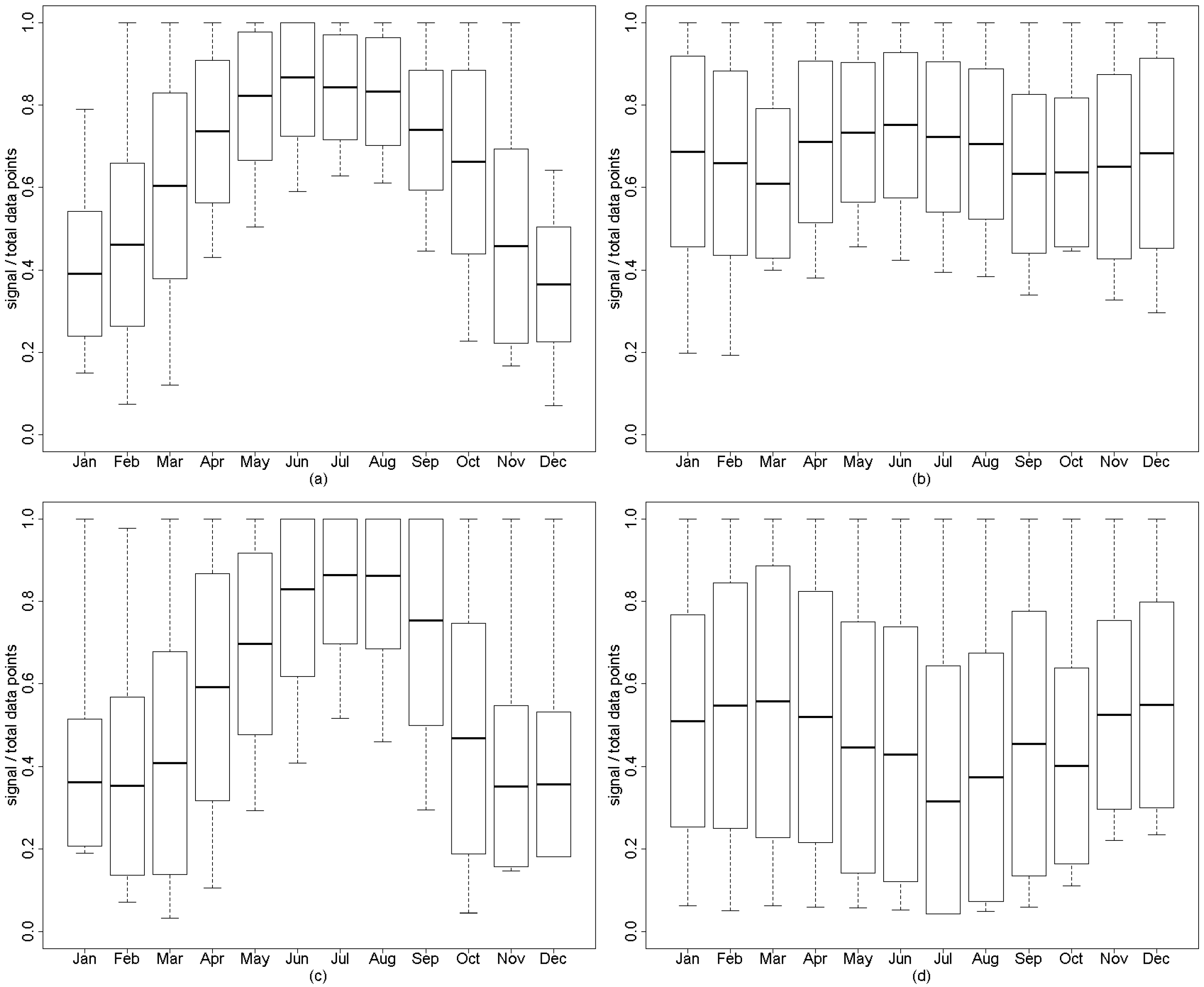
The quality of the interpolated archive is reported on three levels [23]. The first one targets errors in the spatial structure of the interpolated surfaces, as measured by the ratio of the signal (i.e., the number of data points actually used in the interpolation, an indicator of the degrees of freedom associated with each surface) to the total number of data points. In a model with very high goodness-of-fit, it should be about 0.5, but 0.40 and 0.80 are acceptable limits. Higher values indicate either insufficient data or short range correlation in the data values [24,29]. In this archive, this ratio ranged from 0.36 to 0.88 (Figure 2), which in general indicates valid smoothing [15]. Approximately 18% of the surfaces yielded a ratio over 0.8, indicating wide spatial variability or lack of adequate data. This is compatible with low density and sparse distribution of stations in some cases.
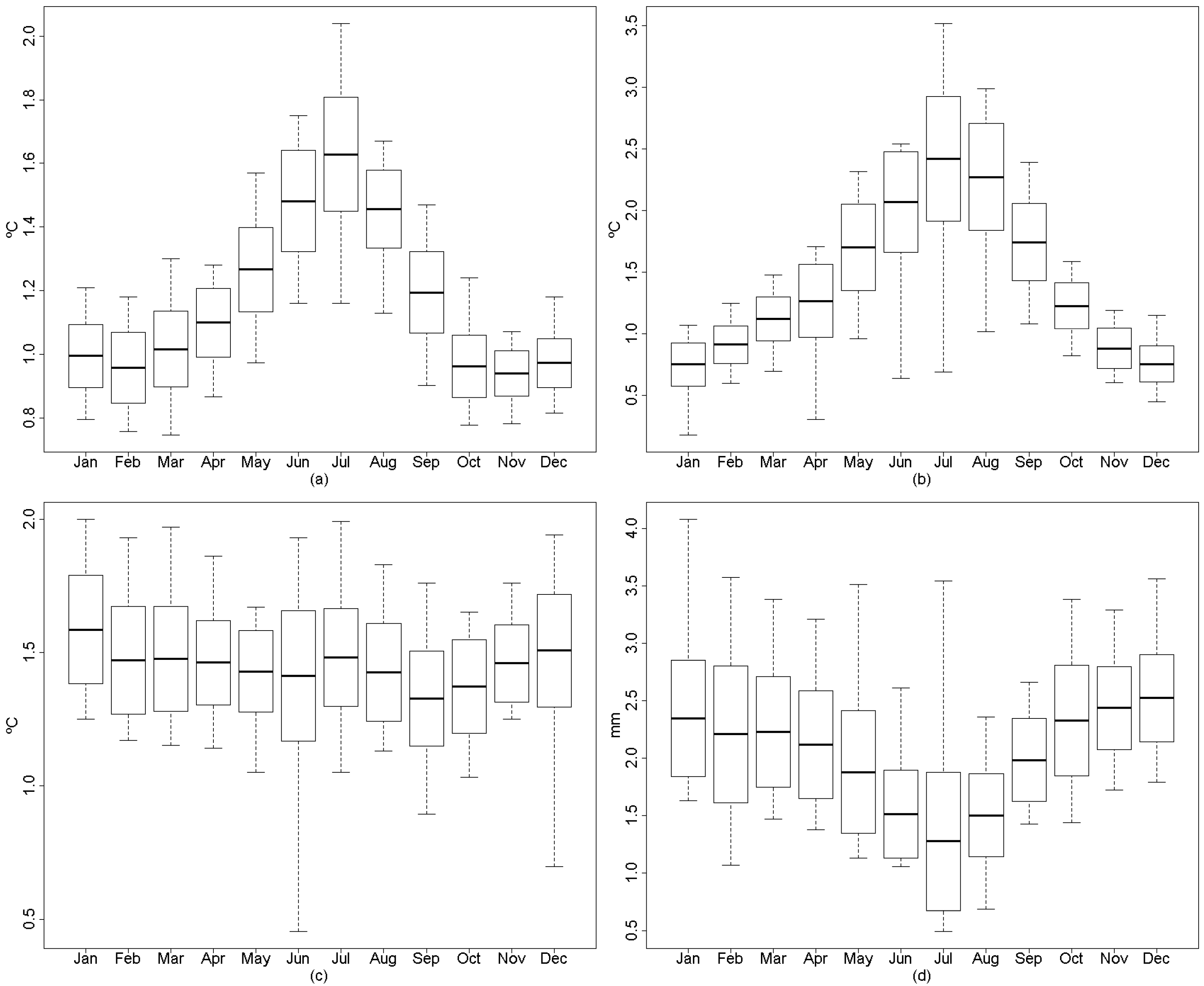
The second estimator of quality targets the predictive error of the interpolated surfaces (Figure 3). The square root of GCV (RTGCV) is an absolute error in the original units of the variable. This was less than 1.5 °C for mean and mean minimum temperatures, but peaked up to 2.5 °C for mean maximum temperatures in the summer months. For precipitation surfaces, RTGCV ranged from 1.2 to 2.5 mm. However it is more meaningful to divide it by the mean, resulting in a relative error. This was below 10% in general, but very low precipitation in the summer months caused it to rise to 40% in July.
Finally, the output archive also includes an error surface per interpolated surface. This represents a Bayesian estimate of the standard error of the model, and can be used to assess the spatial distribution of interpolation errors, for example in error propagation exercises. This set of surfaces is not provided with the main dataset. However, it may be requested by writing to the corresponding author.
The uncertainty associated with each layer is comprised of several different errors: in individual stations data, in spatial configuration of input data points, and in spline fitting. Individual station errors are difficult to track, although the filtering criteria described above are expected to keep quality regular in the general input dataset. Such filters caused spatial arrangements of input data points to vary from month to month, yielding generally higher densities in the more populated zones in the north of the study area. Because such zones also have a more complex topography (related to the Atlas mountain ranges), this bias at least worked in favour of connecting topography and data density. In view of the errors reported, and after visual inspection, we believe the archive successfully captures climate variations associated with large-to-medium geographic gradients. This includes the dominant aridity gradient increasing in the S and SE direction, as well as the breaking points marked by the system of Atlas mountain ranges. It also shows topographic effects linked to kilometric relief mesoforms: altitude, aspect and orientation with respect to prevailing winds. However, thermal inversion in smaller depressions, and in general any microclimate feature of hectometric size or smaller, which lacks a meteorological station to support interpolation, should not be expected to be properly reflected on the surfaces.

4. User Notes

The monthly surfaces are compressed in four independent zip files, one per variable. The decompressed raster layers can be directly imported by several GIS packages or converted to the required GIS format using the gdal_translate utility program [30].
The following tasks depend to a great extent on whether enhanced time-series or period summaries are required. A typical database sequence involves organizing a series of layers, computing new compound serial variables, and finally deriving period summaries. Examples of some tools are given below.
For general work, all the above tasks may be performed with the R package raster [31] which provides several functions for building and managing stacks and raster-layer bricks, which suit the nature of the series of variables well.
Many studies of yearly drylands climate variations use an aridity index based on comparison of precipitation with Potential Evapotranspiration (PET). The r2dRue R package [32] has several utilities for exploiting climate surface time series in this vein. Especially relevant functions are:
  • petHgsm to compute one layer of Potential Evapotranspiration (PET) from tmax, tmed, tmin and extraterrestrial solar radiation layers (internally computed) using the Hargreaves-Samani method [19]. The sister function batchpetHgsm does the same, but for a specified sequence of layers.
  • aiObsMe to compute the FAO-UNEP aridity index as the precipitation ratio to PET for a sequence of layers.
  • rgf.summary to query a sequence of layers and save the resulting summary in a new layer. This summary refers to the population of each grid cell in the specified sequence. Choices are sum, maximum, minimum, mean, count, range, standard deviation, variance and median. The length of the sequences is controlled by the argument step.
These programs are appropriate for building up a climate atlas for the whole period or a subset of it. It can be completed with compound descriptive variables to meet a variety of research goals. For example, the biovars function in the R package dismo [22] uses period summaries of the four basic variables (tmax, tmin, tmed and rain) to generate a set of 19 bioclimatic variables that describe most of the climate variation (mean annual temperature, maximum temperature of the warmest month, precipitation of the warmest quarter, etc.). Such an enhanced atlas can be used for descriptive purposes, or as input data for further modelling (e.g., species distribution models).
All the programs cited in this section are free open source software.

Acknowledgments

This dataset was constructed with funding from the following projects: DeSurvey IP (European Commission FP6 contract No. 003950), MesoTopos (Junta de Andalucia PE P08-RNM-04023) and MELODIES (European Commission FP7, contract No. 603525). The latter also covered the open access publishing costs. Two anonymous reviewers made constructive comments and suggestions that improved the manuscript.

Author Contributions

Alberto Ruiz assembled the input database and performed the spatial interpolations. Maria E. Sanjuan designed the experimental framework and made the geographic validation. Juan Pugdefabregas advised on the archive usability requirements, and edited the manuscript. Gabriel del Barrio assessed spatial errors and wrote the manuscript.

Conflicts of Interest

The authors declare they have no conflict of interest. The funding sponsors had no role in the design of the study; in the collection, analyses, or interpretation of data; in the writing of the manuscript, or in the decision to publish the results.

Abbreviations

The following abbreviations are used in this manuscript:
EPSG
European Petroleum Survey Group
FAO
Food and Agriculture Organization of the United Nations
GCV
Generalized Cross Validation error
GCOS
Global Climate Observing System
GHCN-Monthly
Global Historical Climatology Network-Monthly
GSOD
Global Surface Summary of the Day
NCEI
National Centers for Environmental Information
netCDF
Network Common Data Form
NPP
Net Primary Productivity
PET
Potential Evapotranspiration
RTGCV
Square Root of GCV
UNCCD
United Nations Convention to Combat Desertification
UNEP
United Nations Environment Program
WMO
World Meteorological Organization

References

  1. NCEI. Global Surface Summary of Day, Version 7. National Centers for Environmental Information, NESDIS, NOAA, US Department of Commerce: Asheville, NC, 2016. [Google Scholar]
  2. Hijmans, R.J.; Cameron, S.E.; Parra, J.L.; Jones, P.G.; Jarvis, A. Very high resolution interpolated climate surfaces for global land areas. Int. J. Climatol. 2005, 25, 1965–1978. [Google Scholar] [CrossRef]
  3. Sun, B.; Gao, Z.; Li, Z.; Wang, H.; Li, X.; Wang, B.; Wu, J. Dynamic and dry/wet variation of climate in the potential extent of desertification in China during 1981–2010. Environ. Earth Sci. 2015, 73, 3717–3729. [Google Scholar] [CrossRef]
  4. Durao, R.M.; Pereira, M.J.; Costa, A.C.; Delgado, J.; del Barrio, G.; Soares, A. Spatial-temporal dynamics of precipitation extremes in southern Portugal: A geostatistical assessment study. Int. J. Climatol. 2010, 30, 1526–1537. [Google Scholar] [CrossRef] [Green Version]
  5. Ibrahim, Y.Z.; Balzter, H.; Kaduk, J.; Tucker, C.J. Land degradation assessment using residual trend analysis of GIMMS NDVI3g, soil moisture and rainfall in Sub-Saharan West Africa from 1982 to 2012. Remote Sens. 2015, 7, 5471–5494. [Google Scholar] [CrossRef]
  6. Belbin, L. Environmental representativeness - Regional partitioning and reserve selection. Biol. Conserv. 1993, 66, 223–230. [Google Scholar] [CrossRef]
  7. Almazroui, M.; Dambul, R.; Islam, M.N.; Jones, P.D. Principal components-based regionalization of the Saudi Arabian climate. Int. J. Climatol. 2015, 35, 2555–2573. [Google Scholar] [CrossRef]
  8. Pearson, R.G.; Dawson, T.P.; Liu, C. Modelling species distributions in Britain: A hierarchical integration of climate and land-cover data. Ecography 2004, 27, 285–298. [Google Scholar] [CrossRef]
  9. Tayyebi, A.; Darrel Jenerette, G. Increases in the climate change adaption effectiveness and availability of vegetation across a coastal to desert climate gradient in metropolitan Los Angeles, CA, USA. Sci. Total Environ. 2016, 548–549, 60–71. [Google Scholar] [CrossRef] [PubMed]
  10. Dee, D.P.; Uppala, S.M.; Simmons, A.J.; Berrisford, P.; Poli, P.; Kobayashi, S.; Andrae, U.; Balmaseda, M.A.; Balsamo, G.; Bauer, P.; et al. The ERA-Interim reanalysis: Configuration and performance of the data assimilation system. Q. J. R. Meteorol. Soc. 2011, 137, 553–597. [Google Scholar] [CrossRef]
  11. Rohde, R.; Muller, R.A.; Jacobsen, R.; Muller, E.; Perlmutter, S.; Rosenfeld, A.; Wurtele, J.; Groom, D.; Wickham, C. A new estimate of the average earth surface land temperature spanning 1753 to 2011. Geoinform. Geostat. An Overv. 2013, 1, 1–7. [Google Scholar]
  12. Jones, P.D.; Lister, D.H.; Osborn, T.J.; Harpham, C.; Salmon, M.; Morice, C.P. Hemispheric and large-scale land-surface air temperature variations: An extensive revision and an update to 2010. J. Geophys. Res. D Atmos. 2012, 117, D05127. [Google Scholar] [CrossRef] [Green Version]
  13. Klein Tank, A.M.G.; Wijngaard, J.B.; Können, G.P.; Böhm, R.; Demarée, G.; Gocheva, A.; Mileta, M.; Pashiardis, S.; Hejkrlik, L.; Kern-Hansen, C.; et al. Daily dataset of 20th-century surface air temperature and precipitation series for the European Climate Assessment. Int. J. Climatol. 2002, 22, 1441–1453. [Google Scholar] [CrossRef]
  14. Hutchinson, M.F. Interpolating mean rainfall using thin-plate smoothing splines. Int. J. Geogr. Inf. Syst. 1995, 9, 385–403. [Google Scholar] [CrossRef]
  15. McKenney, D.W.; Pedlar, J.H.; Papadopol, P.; Hutchinson, M.F. The development of 1901–2000 historical monthly climate models for Canada and the United States. Agric. Forest Meteorol. 2006, 138, 69–81. [Google Scholar] [CrossRef]
  16. Yan, H.; Nix, H.A.; Hutchinson, M.F.; Booth, T.H. Spatial interpolation of monthly mean climate data for China. Int. J. Climatol. 2005, 25, 1369–1379. [Google Scholar]
  17. Del Barrio, G.; Puigdefabregas, J.; Sanjuan, M.E.; Stellmes, M.; Ruiz, A. Assessment and monitoring of land condition in the Iberian Peninsula, 1989–2000. Remote Sens. Environ. 2010, 114, 1817–1832. [Google Scholar] [CrossRef]
  18. Del Barrio, G.; Sanjuan, M.E.; Hirche, A.; Puigdefabregas, J.; Yassin, M.; Ruiz, A.; Ouessar, M.; Martinez Valderrama, J.; Essifi, B. Land degradation states and trends in north-western Maghreb drylands, 1998–2008. Remote Sens. under review.
  19. Hargreaves, G.H.; Samani, Z.A. Estimating potential evapotranspiration. J. Irrig. Drain. Div. ASCE 1982, 108, 225–230. [Google Scholar]
  20. UNEP. World Atlas of Desertification, 2nd ed.; UNEP: Nairobi, Kenya, 1992. [Google Scholar]
  21. Xu, T.B.; Hutchinson, M.F. ANUCLIM version 6.1 User Guide; Fenner School of Environment and Society: Canberra, Australia, 2016; p. 90. [Google Scholar]
  22. Hijmans, R.J.; Phillips, S.; Leathwick, J.; Elith, J. dismo: Species Distribution Modeling. R package version 1.0–12. http://CRAN.R-project.org/package=dismo (accessed on 26 June 2016).
  23. Hutchinson, M.F.; Xu, T.B. ANUSPLIN version 4.4 user guide; Fenner School of Environment and Society: Canberra, Australia, 2013. [Google Scholar]
  24. Hutchinson, M.F.; Gessler, P.E. Splines—more than just a smooth interpolator. Geoderma 1994, 62, 45–67. [Google Scholar] [CrossRef]
  25. Jarvis, C.H.; Stuart, N. A comparison among strategies of interpolating maximum and minimum daily air temperatures. Part I: The selection of "guiding" topographic and land cover variables. J. Appl. Meteorol. 2001, 40, 1060–1074. [Google Scholar] [CrossRef]
  26. Lawrimore, J.H.; Menne, M.J.; Gleason, B.E.; Williams, C.N.; Wuertz, D.B.; Vose, R.S.; Rennie, J. An overview of the Global Historical Climatology Network monthly mean temperature data set, version 3. J. Geophys. Res. D Atmos. 2011, 116. [Google Scholar] [CrossRef]
  27. WMO. Guide to Climatological Practices (WMO-No. 100); World Meteorological Organization: Geneva, Switzerland, 2011; p. 115. [Google Scholar]
  28. GCOS. Guideline for the Generation of Datasets and Products Meeting GCOS Requirements GCOS-143 (WMO/TD No. 1530); World Meteorological Organization: Geneva, Switzerland, 2010; p. 10. [Google Scholar]
  29. Hutchinson, M.F. Interpolation of rainfall data with thin plate smoothing splines. Part I: Two dimensional smoothing of data with short range correlation. J. Geogr. Inf. Decis. Anal. 1998, 2, 139–151. [Google Scholar]
  30. GDAL. Geospatial Data Abstraction Library. http://www.gdal.org/ (accessed on 26 June 2016).
  31. Hijmans, R.J. raster: Geographic Data Analysis and Modeling. R package version 2.4–15. http://CRAN.R-project.org/package=raster (accessed on 26 June 2016).
  32. Ruiz, A.; Sanjuan, M.E.; del Barrio, G.; Puigdefabregas, J. r2dRue: 2d Rain Use Efficience library. R package version 1.0.4. http://CRAN.R-project.org/package=r2dRue (accessed on 26 June 2016).
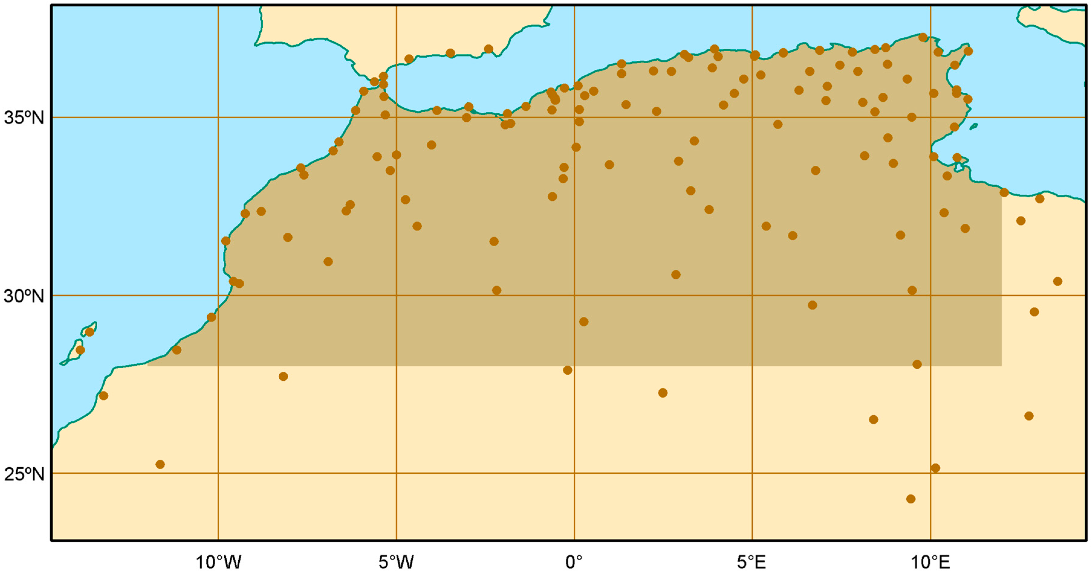
Figure 1. Working window used for interpolation, with the distribution of meteorological stations. The area covered by the final archive (darker frame) is smaller to prevent edge effects.
Data 01 00008 g001
Figure 2. Ratios of the signal to the total number of data points on the interpolated surfaces. Means, standard deviations and extremes shown by months across the climate archive: (a) Mean temperature; (b) Mean maximum temperature; (c) Mean minimum temperature; (d) Precipitation.
Data 01 00008 g002
Figure 3. Absolute errors of the interpolated surfaces Means, standard deviations and extremes shown by months across the climate archive: (a) Mean temperature; (b) Mean maximum temperature; (c) Mean minimum temperature; (d) Precipitation.
Data 01 00008 g003
Table 1. Maghreb climate archive metadata.
FieldValueObservations
file formatnetCDF ‘classic’
data typeinteger
file typebinary
columns2882
rows1320
ref. systemlatlongGeodetic coordinates in WGS84 datum (EPSG code: 4326)
ref. unitsdegreesThe units used to specify position in the layers
min. X−11.9924701
max. X12.0145889
min. Y27.9983998
max. Y38.9939993
resolution0.0083300Equivalent to 925.63 m in a maximum circle
scaling factor0.01Number which multiplies layer values to yield T or P
min. valuee.g.,: −1286Must be rescaled: −1286 × scaling factor = −12.86
max. valuee.g.,: 1314Must be rescaled: 1314 × scaling factor = 13.14
value units°C or mmTemperature or precipitation respectively
flag value−32768Used to mask sea and background areas