

Modelling the Ki67 Index in Synthetic HE-Stained Images Using Conditional StyleGAN Model

 , , , and
Abstract
1. Introduction
2. Background
2.1. Generative Adversarial Networks
2.2. Related Work
3. Methods
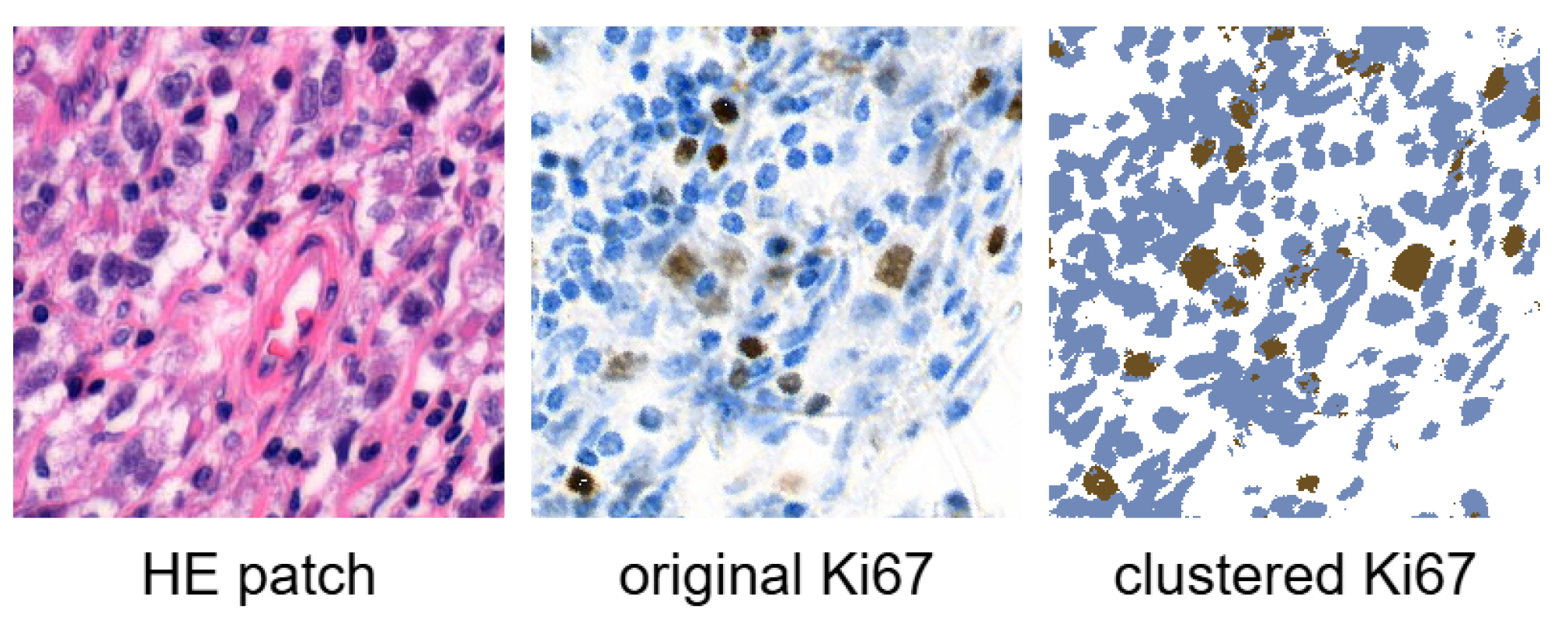
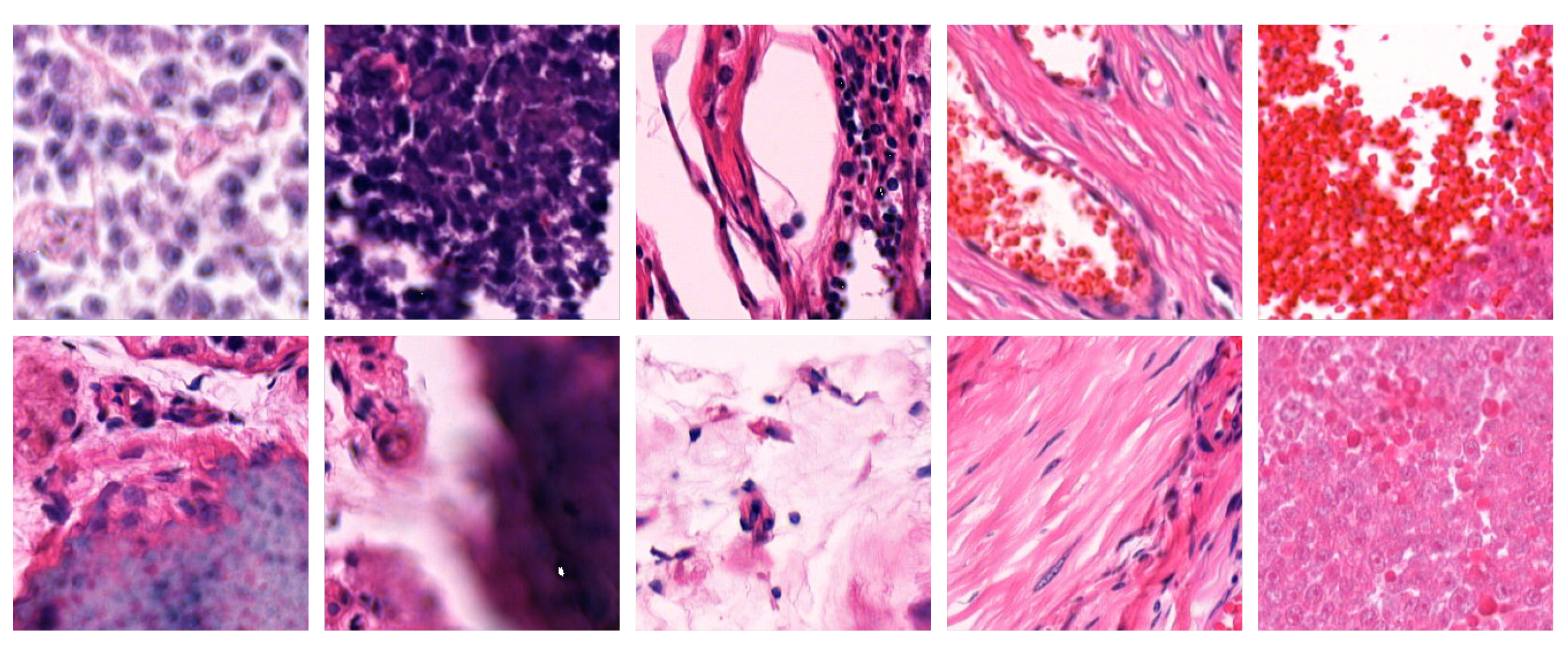
3.1. Dataset
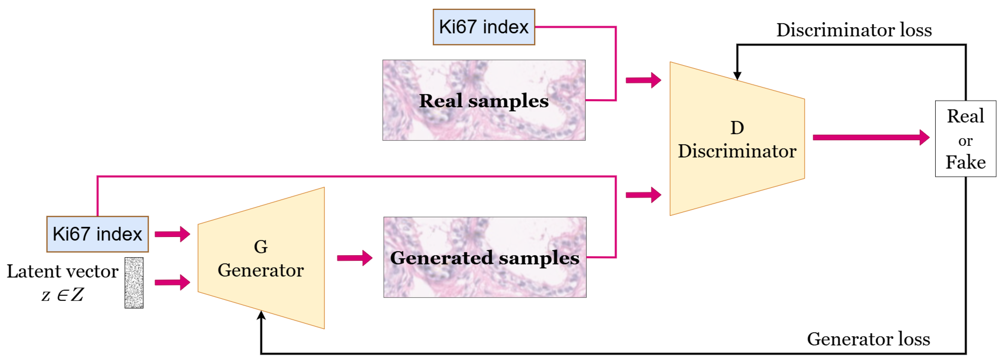
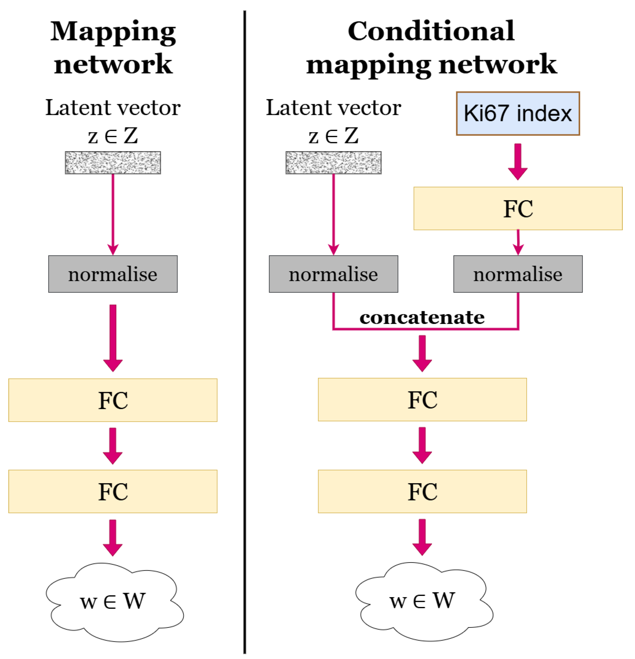
3.2. Generative Model
3.3. Evaluation Metrics
4. Results
4.1. Analysis of Training Progress
4.2. Evaluation of the Conditional Generator
4.2.1. Evaluation Using Fréchet Inception Distance
4.2.2. Evaluation Using Fréchet Histological Distance
4.2.3. Evaluation Using Perceptual Path Length
4.2.4. Discussion
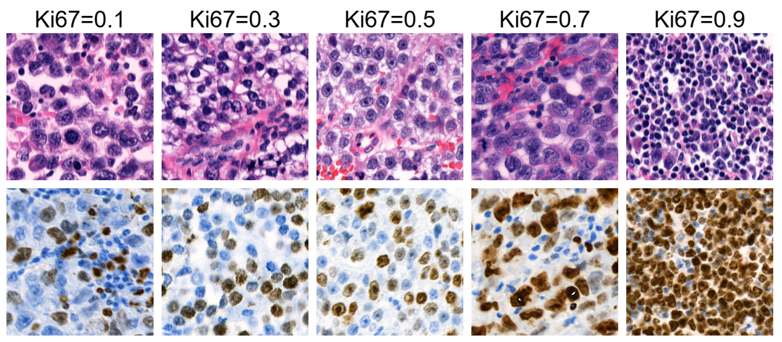
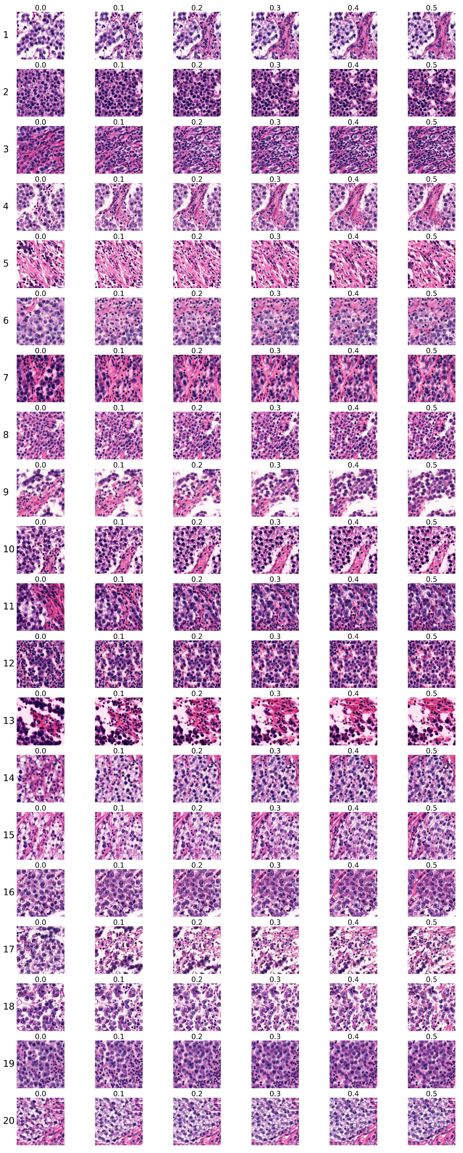
4.3. Analysis of Ki67 Expression in HE-Stained Images
- Each sequence contained six images.
- Images within each sequence were generated from the same randomly selected input latent vector, while the input latent vector differed between sequences.
- The Ki67 index started at Ki67 = 0 for the first image and increased to Ki67 = , with a step size of .
4.3.1. Analysis of the First Group of Sequences
4.3.2. Analysis of the Second Group of Sequences
4.3.3. Discussion
5. Conclusions
Author Contributions
Funding
Institutional Review Board Statement
Informed Consent Statement
Data Availability Statement
Conflicts of Interest
Abbreviations
| FHD | Fréchet Histological Distance |
| FID | Fréchet Inception Distance |
| GAN | Generative Adversarial Network |
| GDPR | General Data Protection Regulation |
| HE | Hematoxylin and Eosin |
| IHC | Immunohistochemical |
| PPL | Perceptual Path Length |
| PSPStain | Pathological Semantics-Preserving Learning method for Virtual Staining |
Appendix A. Heatmap Tables for Ki67 Intervals

| Generator | ||||||||
|---|---|---|---|---|---|---|---|---|
| <0.5,1> | <0,0.5) | |||||||
| <0.2,0.5) | <0,0.2) | |||||||
| Dataset | <0.1,0.2) | <0,0.1) | ||||||
| <0.5,1> | 15.16 | 19.10 | 16.45 | 19.85 | 17.18 | 20.52 | ||
| <0,0.5) | 19.72 | 5.67 | 9.80 | 5.52 | 7.13 | 5.59 | ||
| <0.2,0.5) | 20.50 | 8.17 | 9.90 | 8.42 | 9.45 | 8.57 | ||
| <0,0.2) | 22.12 | 5.45 | 10.26 | 5.59 | 7.24 | 5.65 | ||
| <0.1,0.2) | 19.53 | 6.52 | 8.76 | 6.59 | 6.61 | 7.01 | ||
| <0,0.1) | 20.77 | 5.86 | 10.75 | 5.67 | 7.72 | 5.64 | ||
| Generator | ||||||||
|---|---|---|---|---|---|---|---|---|
| <0.5,1> | <0,0.5) | |||||||
| <0.2,0.5) | <0,0.2) | |||||||
| Dataset | <0.1,0.2) | <0,0.1) | ||||||
| <0.5,1> | 32.41 | 43.08 | 33.39 | 45.68 | 37.62 | 47.95 | ||
| <0,0.5) | 45.40 | 10.36 | 19.85 | 10.41 | 12.95 | 10.83 | ||
| <0.2,0.5) | 35.47 | 23.42 | 20.71 | 25.70 | 22.31 | 26.67 | ||
| <0,0.2) | 44.97 | 10.49 | 21.05 | 10.45 | 13.70 | 10.77 | ||
| <0.1,0.2) | 37.01 | 15.28 | 17.56 | 16.51 | 13.07 | 17.83 | ||
| <0,0.1) | 47.78 | 11.32 | 23.86 | 11.14 | 15.31 | 11.03 | ||
| Dataset | ||||||||
|---|---|---|---|---|---|---|---|---|
| <0.5,1> | <0,0.5) | |||||||
| <0.2,0.5) | <0,0.2) | |||||||
| Dataset | <0.1,0.2) | <0,0.1) | ||||||
| <0.5,1> | 0.00 | 40.95 | 31.47 | 44.38 | 32.75 | 47.80 | ||
| <0,0.5) | 40.95 | 0.00 | 12.82 | 0.30 | 6.19 | 0.87 | ||
| <0.2,0.5) | 31.47 | 12.82 | 0.00 | 16.81 | 9.43 | 19.56 | ||
| <0,0.2) | 44.38 | 0.30 | 16.81 | 0.00 | 7.72 | 0.24 | ||
| <0.1,0.2) | 32.75 | 6.19 | 9.43 | 7.72 | 0.00 | 10.58 | ||
| <0,0.1) | 47.80 | 0.87 | 19.56 | 0.24 | 10.58 | 0.00 | ||
| Generator | ||||||||
|---|---|---|---|---|---|---|---|---|
| <0.5,1> | <0,0.5) | |||||||
| <0.2,0.5) | <0,0.2) | |||||||
| Generator | <0.1,0.2) | <0,0.1) | ||||||
| <0.5,1> | 0.42 | 33.87 | 13.11 | 38.12 | 29.10 | 41.70 | ||
| <0,0.5) | 33.87 | 0.45 | 9.99 | 0.70 | 3.27 | 1.05 | ||
| <0.2,0.5) | 13.11 | 9.99 | 0.44 | 12.92 | 5.72 | 15.35 | ||
| <0,0.2) | 38.12 | 0.70 | 12.92 | 0.44 | 4.41 | 0.61 | ||
| <0.1,0.2) | 29.10 | 3.27 | 5.72 | 4.41 | 0.42 | 6.00 | ||
| <0,0.1) | 41.70 | 1.05 | 15.35 | 0.61 | 6.00 | 0.44 | ||
| <0,1> | ||||||
|---|---|---|---|---|---|---|
| <0.5,1> | <0,0.5) | |||||
| <0.2,0.5) | <0,0.2) | |||||
| <0.1,0.2) | <0,0.1) | |||||
| 1526.11 | 1561.95 | 1549.54 | 1496.20 | 1533.52 | 1482.50 | 1559.26 |
References
- Gurcan, M.N.; Boucheron, L.E.; Can, A.; Madabhushi, A.; Rajpoot, N.M.; Yener, B. Histopathological image analysis: A review. IEEE Rev. Biomed. Eng. 2009, 2, 147–171. [Google Scholar] [CrossRef] [PubMed]
- Band, S.S.; Yarahmadi, A.; Hsu, C.C.; Biyari, M.; Sookhak, M.; Ameri, R.; Dehzangi, I.; Chronopoulos, A.T.; Liang, H.W. Application of explainable artificial intelligence in medical health: A systematic review of interpretability methods. Inform. Med. Unlocked 2023, 40, 101286. [Google Scholar] [CrossRef]
- Regulation, G.D.P. Art. 22 GDPR. Automated individual decision-making, including profiling. Intersoft Consult. 2020, 2. Available online: https://gdpr-info.eu/art-22-gdpr (accessed on 20 April 2023).
- Evans, T.; Retzlaff, C.O.; Geißler, C.; Kargl, M.; Plass, M.; Müller, H.; Kiehl, T.R.; Zerbe, N.; Holzinger, A. The explainability paradox: Challenges for xAI in digital pathology. Future Gener. Comput. Syst. 2022, 133, 281–296. [Google Scholar] [CrossRef]
- Mekala, R.R.; Pahde, F.; Baur, S.; Chandrashekar, S.; Diep, M.; Wenzel, M.; Wisotzky, E.L.; Yolcu, G.Ü.; Lapuschkin, S.; Ma, J.; et al. Synthetic Generation of Dermatoscopic Images with GAN and Closed-Form Factorization. arXiv 2024, arXiv:2410.05114. [Google Scholar]
- Piatriková, L.; Cimrák, I.; Petríková, D. Generation of H&E-Stained Histopathological Images Conditioned on Ki67 Index Using StyleGAN Model. In Proceedings of the 17th International Joint Conference on Biomedical Engineering Systems and Technologies—BIOINFORMATICS, Rome, Italy, 20–22 February 2024; INSTICC; SciTePress: Lisbon, Portugal, 2024; pp. 512–518. [Google Scholar] [CrossRef]
- Piatriková, L.; Cimrák, I.; Petríková, D. Hematoxylin and Eosin Stained Images Artificially Generated by StyleGAN Model Conditioned on Immunohistochemical Ki67 Index. Commun. Comput. Inf. Sci. 2025, in press.
- Goodfellow, I.; Pouget-Abadie, J.; Mirza, M.; Xu, B.; Warde-Farley, D.; Ozair, S.; Courville, A.; Bengio, Y. Generative adversarial nets. Adv. Neural Inf. Process. Syst. 2014, 27, 2672–2680. [Google Scholar]
- Ding, Z.; Jiang, S.; Zhao, J. Take a close look at mode collapse and vanishing gradient in GAN. In Proceedings of the 2022 IEEE 2nd International Conference on Electronic Technology, Communication and Information (ICETCI), Online, 27–29 May 2022; IEEE: Piscataway, NJ, USA, 2022; pp. 597–602. [Google Scholar]
- Mirza, M.; Osindero, S. Conditional generative adversarial nets. arXiv 2014, arXiv:1411.1784. [Google Scholar]
- Karras, T.; Laine, S.; Aila, T. A style-based generator architecture for generative adversarial networks. In Proceedings of the IEEE/CVF Conference on Computer Vision and Pattern Recognition, Long Beach, CA, USA, 15–20 June 2019; pp. 4401–4410. [Google Scholar]
- Daroach, G.B.; Yoder, J.A.; Iczkowski, K.A.; LaViolette, P.S. High-resolution Controllable Prostatic Histology Synthesis using StyleGAN. Bioimaging 2021, 11, 103–112. [Google Scholar]
- Daroach, G.B.; Duenweg, S.R.; Brehler, M.; Lowman, A.K.; Iczkowski, K.A.; Jacobsohn, K.M.; Yoder, J.A.; LaViolette, P.S. Prostate cancer histology synthesis using stylegan latent space annotation. In Proceedings of the International Conference on Medical Image Computing and Computer-Assisted Intervention, Singapore, 18–22 September 2022; Springer: Berlin/Heidelberg, Germany, 2022; pp. 398–408. [Google Scholar]
- Quiros, A.C.; Murray-Smith, R.; Yuan, K. PathologyGAN: Learning deep representations of cancer tissue. arXiv 2019, arXiv:1907.02644. [Google Scholar] [CrossRef]
- Brock, A.; Donahue, J.; Simonyan, K. Large scale GAN training for high fidelity natural image synthesis. arXiv 2018, arXiv:1809.11096. [Google Scholar]
- Jolicoeur-Martineau, A. The relativistic discriminator: A key element missing from standard GAN. arXiv 2018, arXiv:1807.00734. [Google Scholar]
- Quiros, A.C.; Murray-Smith, R.; Yuan, K. Learning a low dimensional manifold of real cancer tissue with PathologyGAN. arXiv 2020, arXiv:2004.06517. [Google Scholar]
- Claudio Quiros, A.; Coudray, N.; Yeaton, A.; Sunhem, W.; Murray-Smith, R.; Tsirigos, A.; Yuan, K. Adversarial learning of cancer tissue representations. In Proceedings of the Medical Image Computing and Computer Assisted Intervention—MICCAI 2021: 24th International Conference, Strasbourg, France, 27 September– 1 October 2021; Proceedings, Part VIII 24. Springer: Berlin/Heidelberg, Germany, 2021; pp. 602–612. [Google Scholar]
- Schutte, K.; Moindrot, O.; Hérent, P.; Schiratti, J.B.; Jégou, S. Using StyleGAN for visual interpretability of deep learning models on medical images. arXiv 2021, arXiv:2101.07563. [Google Scholar]
- Chen, F.; Zhang, R.; Zheng, B.; Sun, Y.; He, J.; Qin, W. Pathological semantics-preserving learning for H&E-to-IHC virtual staining. In Proceedings of the International Conference on Medical Image Computing and Computer-Assisted Intervention, Marrakesh, Morocco, 6–10 October 2024. Springer: Berlin/Heidelberg, Germany, 2024; pp. 384–394. [Google Scholar]
- Petríková, D.; Cimrák, I.; Tobiášová, K.; Plank, L. Dataset of Registered Hematoxylin–Eosin and Ki67 Histopathological Image Pairs Complemented by a Registration Algorithm. Data 2024, 9, 100. [Google Scholar] [CrossRef]
- Petríková, D.; Cimrák, I.; Tobiášová, K.; Plank, L. Semi-Automated Workflow for Computer-Generated Scoring of Ki67 Positive Cells from HE Stained Slides. In Bioinformatics; Science and Technology Publications: Setúbal, Portugal, 2023; pp. 292–300. [Google Scholar]
- Karras, T.; Aittala, M.; Laine, S.; Härkönen, E.; Hellsten, J.; Lehtinen, J.; Aila, T. Alias-Free Generative Adversarial Networks. Adv. Neural Inf. Process. Syst. 2021, 34, 852–863. [Google Scholar]
- Karras, T.; Laine, S.; Aittala, M.; Hellsten, J.; Lehtinen, J.; Aila, T. Analyzing and improving the image quality of StyleGAN. In Proceedings of the IEEE/CVF Conference on Computer Vision and Pattern Recognition, Seattle, WA, USA, 13–19 June 2020; pp. 8110–8119. [Google Scholar]
- Heusel, M.; Ramsauer, H.; Unterthiner, T.; Nessler, B.; Hochreiter, S. GANs trained by a two time-scale update rule converge to a local nash equilibrium. Adv. Neural Inf. Process. Syst. 2017, 30, 6629–6640. [Google Scholar]
- Zhang, R.; Isola, P.; Efros, A.A.; Shechtman, E.; Wang, O. The unreasonable effectiveness of deep features as a perceptual metric. In Proceedings of the IEEE Conference on Computer Vision and Pattern Recognition, Salt Lake City, UT, USA, 18–23 June 2018; pp. 586–595. [Google Scholar]
- Fréchet, M. Sur la distance de deux lois de probabilité. In Annales de l’ISUP; Publications de L’Institut de Statistique de L’Université de Paris: Paris, France, 1957; Volume 6, pp. 183–198. [Google Scholar]
- Simonyan, K.; Zisserman, A. Very deep convolutional networks for large-scale image recognition. arXiv 2014, arXiv:1409.1556. [Google Scholar]


| Generator | ||||||||
|---|---|---|---|---|---|---|---|---|
| <0.5,1> | <0,0.5) | |||||||
| <0.2,0.5) | <0,0.2) | |||||||
| Dataset | <0.1,0.2) | <0,0.1) | ||||||
| <0.5,1> | 15.16 | 19.10 | 16.45 | 19.85 | 17.18 | 20.52 | ||
| <0,0.5) | 19.72 | 5.67 | 9.80 | 5.52 | 7.13 | 5.59 | ||
| <0.2,0.5) | 20.50 | 8.17 | 9.90 | 8.42 | 9.45 | 8.57 | ||
| <0,0.2) | 22.12 | 5.45 | 10.26 | 5.59 | 7.24 | 5.65 | ||
| <0.1,0.2) | 19.53 | 6.52 | 8.76 | 6.59 | 6.61 | 7.01 | ||
| <0,0.1) | 20.77 | 5.86 | 10.75 | 5.67 | 7.72 | 5.64 | ||
| Generator | ||||||||
|---|---|---|---|---|---|---|---|---|
| <0.5,1> | <0,0.5) | |||||||
| <0.2,0.5) | <0,0.2) | |||||||
| Dataset | <0.1,0.2) | <0,0.1) | ||||||
| <0.5,1> | 32.41 | 43.08 | 33.39 | 45.68 | 37.62 | 47.95 | ||
| <0,0.5) | 45.40 | 10.36 | 19.85 | 10.41 | 12.95 | 10.83 | ||
| <0.2,0.5) | 35.47 | 23.42 | 20.71 | 25.70 | 22.31 | 26.67 | ||
| <0,0.2) | 44.97 | 10.49 | 21.05 | 10.45 | 13.70 | 10.77 | ||
| <0.1,0.2) | 37.01 | 15.28 | 17.56 | 16.51 | 13.07 | 17.83 | ||
| <0,0.1) | 47.78 | 11.32 | 23.86 | 11.14 | 15.31 | 11.03 | ||
| Generator | ||||||||
|---|---|---|---|---|---|---|---|---|
| <0.5,1> | <0,0.5) | |||||||
| <0.2,0.5) | <0,0.2) | |||||||
| Dataset | <0.1,0.2) | <0,0.1) | ||||||
| <0.5,1> | 0.42 | 33.87 | 13.11 | 38.12 | 29.10 | 41.70 | ||
| <0,0.5) | 33.87 | 0.45 | 9.99 | 0.70 | 3.27 | 1.05 | ||
| <0.2,0.5) | 13.11 | 9.99 | 0.44 | 12.92 | 5.72 | 15.35 | ||
| <0,0.2) | 38.12 | 0.70 | 12.92 | 0.44 | 4.41 | 0.61 | ||
| <0.1,0.2) | 29.10 | 3.27 | 5.72 | 4.41 | 0.42 | 6.00 | ||
| <0,0.1) | 41.70 | 1.05 | 15.35 | 0.61 | 6.00 | 0.44 | ||
| Generator | ||||||||
|---|---|---|---|---|---|---|---|---|
| <0.5,1> | <0,0.5) | |||||||
| <0.2,0.5) | <0,0.2) | |||||||
| Dataset | <0.1,0.2) | <0,0.1) | ||||||
| <0.5,1> | 0.00 | 40.95 | 31.47 | 44.38 | 32.75 | 47.80 | ||
| <0,0.5) | 40.95 | 0.00 | 12.82 | 0.30 | 6.19 | 0.87 | ||
| <0.2,0.5) | 31.47 | 12.82 | 0.00 | 16.81 | 9.43 | 19.56 | ||
| <0,0.2) | 44.38 | 0.30 | 16.81 | 0.00 | 7.72 | 0.24 | ||
| <0.1,0.2) | 32.75 | 6.19 | 9.43 | 7.72 | 0.00 | 10.58 | ||
| <0,0.1) | 47.80 | 0.87 | 19.56 | 0.24 | 10.58 | 0.00 | ||
| <0,1> | ||||||
|---|---|---|---|---|---|---|
| <0.5,1> | <0,0.5) | |||||
| <0.2,0.5) | <0,0.2) | |||||
| <0.1,0.2) | <0,0.1) | |||||
| 1526.11 | 1561.95 | 1549.54 | 1496.20 | 1533.52 | 1482.50 | 1559.26 |
| Sequence Order | Certainly Unreal | Rather Unreal | Partially Real and Unreal | Rather Real | Certainly Real |
|---|---|---|---|---|---|
| 1 | 1 | 2 | |||
| 2 | 1 | 2 | |||
| 3 | 1 2 | ||||
| 4 | 1 2 | ||||
| 5 | 1 2 | ||||
| 6 | 2 | 1 | |||
| 7 | 1 2 | ||||
| 8 | 2 | 1 | |||
| 9 | 2 | 1 | |||
| 10 | 2 | 1 | |||
| 11 | 1 2 | ||||
| 12 | 2 | 1 | |||
| 13 | 1 2 | ||||
| 14 | 2 | 1 | |||
| 15 | 1 | 2 | |||
| 16 | 1 | 2 | |||
| 17 | 1 | 2 | |||
| 18 | 1 2 | ||||
| 19 | 2 | 1 | |||
| 20 | 1 | 2 |
| Distance | Number of Sequences |
|---|---|
| 0 | 7 |
| 1 | 7 |
| 2 | 6 |
| 3 | 0 |
| 4 | 0 |
| Certainly Unreal | Rather Unreal | Partially Real and Unreal | Rather Real | Certainly Real | |
|---|---|---|---|---|---|
| Pathologist 1 | 0 | 3 | 8 | 9 | 0 |
| Pathologist 2 | 2 | 5 | 4 | 6 | 3 |
| Pathologist 1 and 2 | 2 | 8 | 12 | 15 | 3 |
| Sequence Order | Certainly Unreal | Rather Unreal | Partially Real and Unreal | Rather Real | Certainly Real |
|---|---|---|---|---|---|
| 1 | 1 2 | ||||
| 2 | 1 2 | ||||
| 3 | 1 | 2 | |||
| 4 | 2 | 1 | |||
| 5 | 1 2 | ||||
| 6 | 1 | 2 | |||
| 7 | 1 | 2 | |||
| 8 | 2 | 1 | |||
| 9 | 1 2 | ||||
| 10 | 2 | 1 | |||
| 11 | 2 | 1 | |||
| 12 | 2 | 1 | |||
| 13 | 1 | 2 | |||
| 14 | 2 | 1 | |||
| 15 | 1 | 2 | |||
| 16 | 1 | 2 | |||
| 17 | 1 | 2 | |||
| 18 | 1 | 2 | |||
| 19 | 2 | 1 | |||
| 20 | 2 | 1 |
| Distance | Number of Sequences |
|---|---|
| 0 | 4 |
| 1 | 7 |
| 2 | 6 |
| 3 | 2 |
| 4 | 1 |
| Certainly Unreal | Rather Unreal | Partially Real and Unreal | Rather Real | Certainly Real | |
|---|---|---|---|---|---|
| Pathologist 1 | 1 | 6 | 3 | 8 | 2 |
| Pathologist 2 | 3 | 7 | 3 | 2 | 5 |
| Pathologist 1 and 2 | 4 | 13 | 6 | 10 | 7 |
Disclaimer/Publisher’s Note: The statements, opinions and data contained in all publications are solely those of the individual author(s) and contributor(s) and not of MDPI and/or the editor(s). MDPI and/or the editor(s) disclaim responsibility for any injury to people or property resulting from any ideas, methods, instructions or products referred to in the content. |
© 2025 by the authors. Licensee MDPI, Basel, Switzerland. This article is an open access article distributed under the terms and conditions of the Creative Commons Attribution (CC BY) license (https://creativecommons.org/licenses/by/4.0/).
Share and Cite
Piatriková, L.; Tobiášová, K.; Štefák, A.; Petríková, D.; Plank, L.; Cimrák, I. Modelling the Ki67 Index in Synthetic HE-Stained Images Using Conditional StyleGAN Model. Bioengineering 2025, 12, 476. https://doi.org/10.3390/bioengineering12050476
Piatriková L, Tobiášová K, Štefák A, Petríková D, Plank L, Cimrák I. Modelling the Ki67 Index in Synthetic HE-Stained Images Using Conditional StyleGAN Model. Bioengineering. 2025; 12(5):476. https://doi.org/10.3390/bioengineering12050476
Chicago/Turabian StylePiatriková, Lucia, Katarína Tobiášová, Andrej Štefák, Dominika Petríková, Lukáš Plank, and Ivan Cimrák. 2025. "Modelling the Ki67 Index in Synthetic HE-Stained Images Using Conditional StyleGAN Model" Bioengineering 12, no. 5: 476. https://doi.org/10.3390/bioengineering12050476
APA StylePiatriková, L., Tobiášová, K., Štefák, A., Petríková, D., Plank, L., & Cimrák, I. (2025). Modelling the Ki67 Index in Synthetic HE-Stained Images Using Conditional StyleGAN Model. Bioengineering, 12(5), 476. https://doi.org/10.3390/bioengineering12050476